| Issue |
Acta Acust.
Volume 9, 2025
|
|
|---|---|---|
| Article Number | 48 | |
| Number of page(s) | 21 | |
| Section | Auditory Quality of Systems | |
| DOI | https://doi.org/10.1051/aacus/2025031 | |
| Published online | 24 July 2025 | |
Scientific Article
A psychoacoustic assessment for enhancing the sound quality of vibrating composite panels
1
ENTPE, Ecole Centrale de Lyon, CNRS, LTDS, UMR5513 69518 Vaulx-en-Velin France
2
Ecole Centrale de Lyon, CNRS, LTDS, UMR5513 69130 Ecully France
3
LVA, INSA-Lyon, LVA EA677 F-69621 Villeurbanne France
* Corresponding author: This email address is being protected from spambots. You need JavaScript enabled to view it.
Received:
8
November
2024
Accepted:
20
June
2025
Abstract
Vibrating composite panels are widely used in airplanes, vehicles, and high-speed trains, where noise comfort is required. Optimizing their design requires integrating psychoacoustic assessments alongside vibroacoustic analysis. The research presents a psychoacoustic framework to enhance the sound quality of composite panels while maintaining their structural efficiency. Hence, vibroacoustic models previously validated through vibroacoustic laboratory experiments for various composite panels subjected to mechanical and diffuse acoustic excitations, were used to synthesize the sounds radiated from the panels. The framework required to validate the models perceptually. This ensured the synthesized sounds were perceived by listeners as equivalent to the recorded ones. A psychoacoustic paired-comparison test between recorded and synthesized sounds was conducted to perceptually assess the modeling. Next, the sound quality of composite panel designs was investigated. Hence, synthesized sounds of designs were evaluated through another psychoacoustic test and a preference analysis. The preference analysis identified optimal designs, correlating preferences with psychoacoustic indices, like loudness, and mechanical properties such as stiffness-to-mass ratio and damping. This integrated approach ensures that the resulting designs enhance the sound quality and meet structural performance requirements.
Key words: Composite / Vibroacoustic / Psychoacoustic / Auditory evaluation / Design
© The Author(s), Published by EDP Sciences, 2025
 This is an Open Access article distributed under the terms of the Creative Commons Attribution License (https://creativecommons.org/licenses/by/4.0), which permits unrestricted use, distribution, and reproduction in any medium, provided the original work is properly cited.
1 Introduction
Nowadays high-tech industries, such as aerospace and high-speed transportation, increasingly use composite structures due to their exceptional mechanical properties (see [1, 2]). A composite sandwich panel, as a common composite structure, features two thin, stiff face sheets and a thick, lightweight core. The face sheets provide strength and stiffness, while the core sustains transverse shear loads (see [3]). Another common composite structure is the laminate panel, made by bonding layers of materials such as carbon fiber-reinforced polymers (CFRPs) with epoxy resin (see [4]).
Research on the vibroacoustic behaviors of composite panels began in the late 20th century, with studies on various excitations [5]. Recent research on composite panels largely emphasizes mechanical and vibroacoustic properties, often overlooking psychoacoustics. However, in enclosed spaces like vehicles and airplanes, where noise from vibrating composite structures affects passengers, integrating psychoacoustic considerations is crucial. Nowadays, a growing trend incorporates psychoacoustic analysis across various engineering fields, such as aircraft system design [6–9], automotive engineering and vehicle design [10–12], rotating machine monitoring [13], transportation [14, 15], home appliances [16], and building acoustics [17, 18]. Meanwhile, psychoacoustic assessments of composite materials have mainly been limited to musical instrument studies, such as a development of a composite guitar with carbon fiber reinforced polyurethane foam [19] and an evaluation of acoustic properties in prototype violins [20].
Although psychoacoustic studies on composite panels have been overlooked in engineering, research on isotropic structures exists. For example, Meunier et al. [21] analyzed vibroacoustic and psychoacoustic responses of vibrating plates under mechanical or acoustic excitation. Canévet et al. [22] investigated fluid-loaded plates under transient forces, while Demirdjian et al. [23] combined analyses of fluid-loaded, clamped plates. These studies emphasize a psychomechanical approach, showing that mechanical factors such as damping, excitation duration, and force location affect perceptual dimensions like tonalness and sharpness. Faure and Marquis-Favre [24] investigated how parameters like damping and material properties affect sound perception from a simply-supported steel plate excited by a normal incidence plane wave with a white noise spectrum. Demirdjian et al. [25] compared sounds from fluid-loaded plates under transient forces with simulations for clamped steel plates. Both aimed to link mechanical parameters with auditory characteristics. Marquis-Favre and Faure [26] explored the effect of boundary conditions on auditory attributes of thin vibrating panels. Trollé et al. [27] studied the impact of structural parameters of a window on environmental noise perception. They focused on structural parameters and absorption for a system composed of a plate and a cavity, and on optimizing vibroacoustic computations for sound quality evaluation [28]. McAdams et al. [29] simulated sound sources and impacts to relate perceptual dimensions to physical properties. Hjortkjær and McAdams [30] analyzed auditory attributes and categorization of sounds from various materials.
Knowledge from isotropic panels offers a useful foundation, but it is insufficient to capture the structural and material complexities of composite panels. Vibroacoustic modeling of composites like sandwich panels requires higher-order models to address their anisotropic, layered structures and the interactions between facesheets, core, and varying physical properties (e.g., see [31]). The current research advances previous studies on composite panels by integrating psychoacoustic considerations. Building on validated vibroacoustic models (see [31, 32]), a framework was propose in the current study to enhance sound quality of composite panels through three steps: sound synthesis from vibroacoustic models, perceptual validation of the sound synthesis, and design optimization. In the first step, sounds were synthesized using physical models developed in frequency domain and validated through laboratory vibroacoustic experiments in previous works (see [31, 32]). Since these models and the associated synthesis were intended for psychoacoustic assessment of composite panels, their perceptual validation was also necessary. Hence, in the second step, a psychoacoustic test was conducted to validate the synthesized sounds (thus, to validate the models) from the perceptual point of view. Once confirmed as physically and perceptually reliable, the modeling was used in the third step to synthesize sounds for various composite panel designs. Figure 1 illustrates the thick composite sandwich panel, with a Nomex-honeycomb core and CFRP face sheets, studied by AllahTavakoli et al. [31], which served as the inspiration for the designs investigated in the current research. This part of the research investigates two distinct excitations: a mechanical excitation with a localized force on the panel, and a diffuse acoustic field excitation, which applies a spatially uniform sound field. The mechanical excitation excites some structural vibrations, while acoustic excitation activates the entire panel surface, affecting a wider range of frequencies of the vibroacoustic behavior of the panel. This dual approach ensures a comprehensive evaluation of the sound radiated under different real-world conditions, such as localized impacts or external noise sources. Finally, another set of psychoacoustic test and analysis were conducted for the two mechanical and acoustic excitations to evaluate the designs and identify the optimal one based on a psychoacoustic perspective. Figure 2 summarizes these key steps of the current research. The paper is structured as follows: Section 2 presents the methodology of the research, including the sound synthesis and the psychoacoustic tests. Section 3 covers the main results of the research including the results of perceptual validation through psychoacoustic testing and analyses, comparing the synthesized sounds (i.e., simulations) to audio recordings, and the results associated with the design and optimization step to assess composite panel designs and find the optimal ones with the best preference. Finally, Section 4 discusses key findings and concludes the paper.
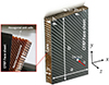 |
Figure 1. The thick composite sandwich panel with a Nomex-honeycomb core and CFRP face sheets, studied by AllahTavakoli et al. [31], from which the designs of the composite panel in the current research was inspired. |
 |
Figure 2. Overview of the steps of the psychoacoustic framework developed for enhancing the sound quality of vibrating composite panels. |
2 Methodology
The methodology in this paper consists of three main steps: sound synthesis, perceptual validation, and design and optimization of the composite panels. Each step involves specific approaches, tests, and analyses that prepare the requirements for the subsequent steps.
2.1 Sound synthesis
Sound synthesis was based on the mathematical modeling of the acoustic pressure field radiated by vibrating composite panels under mechanical and diffuse acoustic excitations. The modeling of the vibrating panels was consistent with established approaches. For thin composite and isotropic plates (e.g., laminates, steel, and aluminum), a fourth-order Kirchhoff-Love model was used, as shear deformation is negligible. For sandwich composites, a sixth-order model captured transverse shear for accurately modeling thick, multilayered panels. The models have been vibroacoustically validated through laboratory experiments, demonstrating strong agreement between simulations and measurements (see [31, 32]), which is summarized below. Consider a vibrating rectangular composite panel of dimensions a×b. Under the Kirchhoff-Love hypothesis, and neglecting transverse shear and rotary inertia, the transverse displacement w satisfies a fourth-order partial differential equation (PDE) used for modeling thin composite plates as follows (e.g., [4, 33]):
 (1)
(1)
where ![Mathematical equation: $ (x,y)\in \left [0,a \right ]\times \left [0,b \right ] $](/articles/aacus/full_html/2025/01/aacus240133/aacus240133-eq2.gif) , t is the time, D11, D22, D12, and D66 are the bending rigidity coefficients, ρ is the mass density, h is the thickness, M=ρh is the mass per unit area, and and q is the external force. However, in composite panels like sandwiches, where shear effects are significant, the equations of motion may be higher-order problems, such as the sixth-order problem incorporating shear effects, as shown below (e.g., [31, 34]):
, t is the time, D11, D22, D12, and D66 are the bending rigidity coefficients, ρ is the mass density, h is the thickness, M=ρh is the mass per unit area, and and q is the external force. However, in composite panels like sandwiches, where shear effects are significant, the equations of motion may be higher-order problems, such as the sixth-order problem incorporating shear effects, as shown below (e.g., [31, 34]):
 (2)
(2)
where ∇6(•)=∇2(∇2(∇2(•))), ∇4(•)=∇2(∇2(•)),  is the Laplacian operator,
  is the shear parameter, G is the shear modulus, Y=3(1+hc/hf)2 is the geometric parameter, Dt is the total flexural rigidity, Ef is Young's modulus, ν is the Poisson's ratio, M=ρh is the mass per unit area, ρ is the mass density, hf and hc are the thicknesses of the face sheet and core layer, h=2hf+hc is the total thickness [35]. Consequently, having the transverse displacement w (flexural vibration), Rayleigh integration can be employed to model the acoustic pressure radiated by the vibrating composite plate in a fluid half-space as follows (e.g., [36]):
 (3)
(3)
where Ray is the Rayleigh integration operator. The panel is embedded within a rigid baffle, and the acoustic pressure is considered to be radiated from the panel into a fluid half-space z>0. The pressure field at any location (x,y,z) is denoted by p(x,y,z;ω), where ω is the angular frequency, and ρ0 represents the air density. The differential surface element of the plate is defined as dS′=dx′ dy′, the wave number is  , where c0 is the speed of sound in air, and the distance between points is expressed as
  .
.
Also, when the panel is excited by a random pressure field excitation such as the diffuse acoustic field (DAF), the power spectrum of the sound pressure Sp at the location  can be modeled via the Rayleigh integration as follows (cf. [32, 37]):
 (4)
(4)
 (5)
(5)
where  denotes the complex conjugate,
  is the correlation function of the random pressure field excitation, Spe is the power spectrum of the random excitation, and {Hn} and {ψn} are, respectively, the frequency response function and mode functions of the vibrating panel (see [32, 38]).
Figure 3 illustrates the setups of the vibroacoustic experiments. The mechanical excitation experiment was conducted using a laser vibrometry system with a spectrum analyzer, signal generator, shaker, transducer, microphone, and laser vibrometer [31]. For the DAF excitation, an acoustic cabin with four speakers and a microphone antenna was used to generate and monitor the acoustic field inside the cabin, while a microphone outside the cabin recorded the sound from the vibrating plate [32].
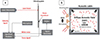 |
Figure 3. The set-up diagram of (a) the mechanical excitation experiment with a laser vibrometer, spectrum analyzer, signal generator, microphone, and shaker (see [31]), and (b) the diffuse acoustic excitation experiment with an acoustic cabin, four speakers, a 4-microphone array inside the cabin, and a microphone outside (see [32]). |
The experimental setups, for both the mechanical and acoustical excitations with white noise stochastic behavior, satisfy key assumptions for using the Rayleigh method, including anechoic boundaries in the anechoic chamber, and a controlled diffuse sound field in an acoustic cabin for producing the acoustic excitation. The compliance with the requirements of the method was verified by comparisons between simulations and measurements of the sound pressure level, thanks to vibroacoustic experiments carried out with mechanical and DAF excitations (cf. [31, 32]). Audio recordings of sound radiation from the vibrating panels were also realized during these vibroacoustic experiments in the perspective of the perceptual validation of the vibroacoustic models and the associated synthesis.
The measurements were acquired in the frequency range [3.125 Hz,10 kHz] for the mechanical excitation, and in the frequency range [1 Hz,10 kHz] for the acoustic excitation. The boundary conditions of the panels were clamped, and all sound recordings from the vibrating plates, for both excitation types, were made 50 cm from the midpoint of the vibrating plates. For these excitations and frequency range, the measurement points were positioned between the near field and far field. Due to the white noise stochastic behavior of the two excitations, the pressure measurements remained stable and repeatable, indicating no influence of potential near-field phenomena. This was confirmed by the good comparison between simulated and measured pressures (cf. [31, 32]). Finally, the synthesized sounds were produced by computing the complex sound pressure in the frequency domain using the Rayleigh integral (see Eqs. (3) and (4)). These results correspond to the discrete Fourier transform (DFT) of the time-domain pressure signal. The inverse Fourier transform was then used to reconstruct the time-domain signal from the DFT coefficients over an arbitrary time interval [39], assuming periodicity and spectral band limitation, which are valid here due to the stationary nature of the signals and the broadband characteristics of the excitations. For the studied vibrating panels, the acoustic energy was concentrated at resonance frequencies significantly higher than the lower bound of the frequency range, with the excitation bandwidth extending up to 10 kHz [31, 32]. No audible periodicity artifacts were observed.
2.2 Perceptual validation
In this step, the psychoacoustic test was conducted to validate the sound synthesis carried out for various material panels, including composite Nomex-core sandwich, CFRP laminate, aluminium composite plate, and steel and aluminium isotropic plates.
2.2.1 Psychoacoustic test
The psychoacoustic test consisted of three sessions. Session 1 dealt with sounds from plates excited by the mechanical point force, Session 2 concerned sounds from plates excited by the DAF, and Session 3 was linked to the objective of optimizing the maximum frequency used for the simulations based on perceptual factors. Session 3 helped us to avoid unnecessary computational effort by eliminating high-frequency components that do not significantly impact the assessment of the panel sounds from a perceptual point of view.
Participants: They were students and staff from ENTPE, the engineering school on the campus site. They declared to have normal hearing, and they were compensated for their participation. In all the psychoacoustic tests of the current research, an informed consent was obtained from all participants in accordance with the Declaration of Helsinki. As the study posed no medical, psychological, or ethical risks, ethics committee approval was not required under national law and the institutional ethical standards. For the step of the perceptual validation, the test involved 40 participants (23 females, 17 males, aged 18–61 yrs, average age 28.9 yrs, SD 12.8 yrs).
Apparatus: The sounds were reproduced using Sennheiser HD600 headphones and a LynxTWO sound card. As specified by the manufacturers, the headphones can accurately reproduce sound from 12 Hz to 39 kHz, while the sound card, with 192 kHz sample rate support, which ensures precise playback, and makes them well-adapted for the listening test. The test was performed in a quiet room at ENTPE with 24 dB(A) background noise. A MATLAB-based interface was developed for participants to acquire their responses. Prior to the listening test, sound reproduction levels were adjusted using a Cortex Manikin MK2 to ensure participant comfort by considering the same decrease in global SPL and keeping the differences observed between the initial simulations.
Stimuli: In Session 1, eight stimuli were used, involving both synthesized (simulated) and the corresponding recorded sounds from four material plates (steel, aluminum, composite laminate, and composite sandwich) with dimensions 40 cm×60 cm under mechanical excitation (cf. Fig. 3a, for the vibroacoustic experiment and modeling, see [31]). Session 2 included six stimuli, simulated and the corresponding recorded sounds from three plates (aluminum, steel, and composite aluminum) with dimensions 33.9 cm×29.2 cm under acoustic excitation (cf. Fig. 3b, see [32]). The panel geometries were chosen to fit the size constraints of the measuring windows in the anechoic chamber and acoustic cabin available for the vibroacoustic experiments. Session 3 involved seven synthesized stimuli with different cutoff frequencies to determine the optimal maximum frequency for simulations. Table 1 displays all the stimuli with the mean A-weighted sound pressure level (SPL) and the properties of panels and simulations. Frequency resolutions were 3.125 Hz for Sessions 1 and 3, and 1 Hz for Session 2. The maximum frequency for all computations was 10 kHz, with specific cutoffs in Session 3 (2 kHz to 7 kHz in 1 kHz increments, see Tab. 1). All stimuli lasted 3 s, with fade-ins and fade-outs of 0.1 s to prevent playback clicks. The duration of these stationary stimuli was fixed based on previous works (e.g., [40]) and out of concern for listener fatigue.
The properties of stimuli: dimensions a×b, thickness h, bending stiffness D, Young's modulus E, Poisson ratio ν, surface mass density M, and loss damping factor η of vibrating panels. fM: cutoff frequency for simulation, SPL: mean A-weighted sound pressure level. “S.”, “No.”, and “Exc.” denote session, stimulus number, and excitation type. “Mech” and “Acous” refer to mechanical and acoustic excitations; “Mic” and “Sim” to microphone-recorded or simulated stimuli.
Procedure: The listening test procedure used here was based on a paired-comparison method, designed by previous studies [41, 42]. The paired-comparison method is well-known to be highly discriminating, and the drawback of this approach is its time consumption when dealing with a large number of stimuli (e.g., see [43–45]). However, the limited number of stimuli per session in this study (see Tab. 1) allowed for capturing all dissimilarity judgments with this method and without excessive participant fatigue. For N stimuli in each session, the paired-comparison method, which also includes comparisons of the same stimuli in pairs, results in  paired sounds as trials for each participant per session. Accordingly, each participant was asked to judge 36, 21, and 28 trials of paired sounds for Session 1, Session 2, and Session 3, respectively. Participants spent an average of 45 min on the psychoacoustic test, including instructions, training, and judgments across three sessions. Sound pairs and their arrangements were randomized to prevent bias, and sessions were presented in a random order to avoid methodological bias regarding excitation type and maximum frequency. Each session began with training to familiarize participants with the sounds, procedures, interface, and response scale. Participants rated sound pairs on a 0 to 10 scale, from “Very similar” (0) to “Very different” (10), with judgments recorded by the interface. Participants were free to replay each pair as often as needed. The test duration was approximately 45 min.
2.2.2 Data analysis
Classification: Classification and dendrograms were used to identify outliers in participant-acquired datasets of the psychoacoustic test. Outliers, differing significantly from the dataset, might not fit into clusters or could form isolated clusters with high score differences. The objective was to ensure consensus in participant judgments before analyzing stimulus dissimilarities. Ascending Hierarchical Classification (AHC), following previous works [41, 42], used linear Bravais–Pearson correlation to measure dissimilarity between participant responses. Aggregation methods examined included Single, Complete, Average, Weighted, Centroid, Median, and Ward linkage, with cophenetic and Goodman–Kruskal coefficients evaluating method adequacy (see [46–48]). The method selected was the one which maximized the cophenetic and Goodman–Kruskal correlation coefficients. Then, from the obtained dendogram, the quality index was calculated to determine the optimal number of classes (e.g., [42, 49]). This final step allowed to point out potential outliers.
Multidimensional scaling: To analyze stimuli dissimilarities and visualize the stimuli in a perceptual space, Individual Differences Scaling (INDSCAL) was used, an MDS algorithm for examining variable relationships based on individual judgments (see [50–53]). INDSCAL reveals perceptual dimensions which may be explained by auditory attributes. The algorithm uses the formula:
![Mathematical equation: $$ d_{jk}^{i}=\left [\sum _{n=1}^{N} w_{n}^{i} \left (x_{jn}-x_{kn} \right )^{2} \right ]^{\frac {1}{2}}. $$](/articles/aacus/full_html/2025/01/aacus240133/aacus240133-eq15.gif) (6)
(6)
Here,  is the dissimilarity between stimuli j and k for participant i, N is the dimensionality of the stimulus space, xjn is the coordinate of stimulus j on the nth dimension, and
  is the participant's weight for that dimension. INDSCAL outputs include a matrix of stimulus coordinates X=[xjn] and a matrix of participant weights
 ![Mathematical equation: $ {\mathbf {W}}=[w_{n}^{i}] $](/articles/aacus/full_html/2025/01/aacus240133/aacus240133-eq18.gif) [52]. We used MATLAB for INDSCAL analysis on dissimilarity data from the three psychoacoustic test sessions. Determining the optimal number of dimensions was critical for model accuracy and complexity. Herein, the L-Curve method was used to balance these factors, employing Scree plots to visualize the trade-off between these two factors (see [53–55]). The L-Curve method, developed for parameter selection in ill-posed problems [56], helps find the point of maximum curvature to optimize multiple objectives [57]. This method indicates the number of dimensions that strike a balance between effective reconstruction (i.e., accurate calculation of dissimilarity) and complexity in the problem-solving process (i.e., number of dimensions) (e.g., see [56]). In addition, the confidence interval for each stimulus, represented as a 2D error ellipse in the perceptual space, as been determined using the bootstrap technique at a 95% confidence level (see [58]).
[52]. We used MATLAB for INDSCAL analysis on dissimilarity data from the three psychoacoustic test sessions. Determining the optimal number of dimensions was critical for model accuracy and complexity. Herein, the L-Curve method was used to balance these factors, employing Scree plots to visualize the trade-off between these two factors (see [53–55]). The L-Curve method, developed for parameter selection in ill-posed problems [56], helps find the point of maximum curvature to optimize multiple objectives [57]. This method indicates the number of dimensions that strike a balance between effective reconstruction (i.e., accurate calculation of dissimilarity) and complexity in the problem-solving process (i.e., number of dimensions) (e.g., see [56]). In addition, the confidence interval for each stimulus, represented as a 2D error ellipse in the perceptual space, as been determined using the bootstrap technique at a 95% confidence level (see [58]).
2.3 Design and optimization
Continuing from the perceptual validation of the modeling of composite panels discussed in the previous section, this step focused on the perceptual aspects of designing and optimizing vibrating composite panels. We first designed composite panels and synthesized their corresponding sounds, based on the model vibroacoustically validated through laboratory experiments [31] and also perceptually validated following the method described in Section 2.2. Then, a psychoacoustic test was conducted to assess the synthesized sounds of the designs from a perceptual standpoint.
2.3.1 Designs
According to [31], an updated model for composite sandwich panels with CFRP face sheets and a Nomex honeycomb core has been developed and physically validated. The method described in Section 2.2 aimed at validating this model from a perceptual point of view. After its perceptual validation, the model can be used to explore various designs with mechanical and geometrical characteristics from a perceptual perspective. Table 2 lists the parameters of the composite sandwich specimen tested in the vibroacoustic experiments of the previous study [31]. Using these as reference values (cf. Tab. 2), the parameters were organized for 10 composite panel designs as shown in Table 3. The parameter ranges were aligned with the reference values and based on recent studies (e.g., [59–67]). In Table 3, parameter variations are independent except for the equivalent parameters – total bending stiffness Dt, equivalent Young modulus Eequi, total surface mass density M, and stiffness-to-mass ratio Dt/M, which are derived from the other parameters. Bending stiffness is calculated using laminate theory and the stiffness matrix, with Eequi derived from Dt=Eequih3/12/(1−ν2), where h=2hf+hc is the total panel thickness and ν is the Poisson ratio. Figure 1 presents the geometrical configuration of the composite sandwich panel.
The composite sandwich panel parameters, tested in vibroacoustic experiments by AllahTavakoli et al. [31]: dimensions a×b, face sheet thickness hf, core thickness hc, and Dt, Ef, G, ν, and η represent the total bending stiffness, Young's modulus of face sheets, core shear modulus, Poisson ratio, and loss damping factor, respectively.
For vibroacoustic modeling of the composite sandwich panel, the updated 6th order model was used to compute the plate vibratory field [31]. The Rayleigh integration in the frequency domain is then used to model the sound pressure field at 50 cm from the panel and synthesize the sounds (cf. Sect. 2.1). The simulation conditions matched those in the experiments described in Figure 3.
2.3.2 Psychoacoustic test
Herein, to conduct the psychoacoustic test aimed at evaluating the composite sandwich panel designs, we adhered to similar protocols and procedures employed in Section 2.2 for the perceptual validation. Additionally, the current test incorporates preference score measurements.
Participants: A total of 40 participants, 22 females and 18 males, from 19 to 63 years (mean = 35.8 yrs, SD = 15.3 yrs), were involved in the test. They were from students and staff from the ENTPE. All participants were engaged in every test session, and received compensation for their involvement in the psychoacoustic test. This study followed the standards of the Declaration of Helsinki (cf. Sect. 2.2). Prior to experiment, each participant confirmed their normal hearing abilities and provided written consent for their participation.
Apparatus: The instrument set-up for this psychoacoustic test was similar to the apparatus described in Section 2.2.
Stimuli: For the 10 composite sandwich panel designs, the psychoacoustic test was carried out in two distinct sessions, each with a specific excitation (cf. Fig. 3). For Session 1, our focus was to assess the preference and psychoacoustic qualities of these designs when subjected to the mechanical excitation. Session 2 involved assessing the designs, subjected to the diffuse acoustic field excitation. Figure 4 illustrates the spectra of the sound pressure level for stimuli 8 and 9, corresponding to the designs with the highest and lowest values of total bending stiffness Dt, respectively (cf. Tab. 3). Also, Table 4 presents the overall sound pressure levels in dB(A) for the synthesized sounds corresponding to the different designs, considering both mechanical and acoustic excitations. Akin to the procedures in Section 2.2, stimuli were adjusted using the Cortex Manikin MK2 to ensure participant comfort. Hereafter, Sessions 1 and 2 shall be referred to as the “mechanical session” and the “acoustic session”, respectively.
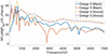 |
Figure 4. The SPL spectra for stimuli 8 and 9, corresponding to designs with the highest and lowest values of total bending stiffness Dt, respectively, under mechanical (labeled as “Mech”) and acoustic (labeled as “Acous”) excitations. |
The sound pressure levels of the stimuli for the designed composite panels excited by the mechanical and acoustic excitations, [unit: dB(A)].
Procedure: To assess designs through psychoacoustic test, the paired-comparison method outlined in Section 2.2 was employed. In the current test, dissimilarity ratings and preference scores were collected. For 10 stimuli in each session, the paired-comparison method, which also includes comparisons of the same stimuli in pairs, results in  paired sounds as trials for each participant per session. The presentation order of sound pairs and their arrangement were randomized. Moreover, sessions were also presented in random order, each beginning with on-screen instructions and a training part to familiarize participants with sounds and the interface. Each session involved listening to sound pairs. The participants were asked to assess the difference between the sounds on a continuous scale from 0 to 10, 11 numerical labels evenly spaced out and 2 with verbal descriptors (“Very similar” and “Very different”). Preference was measured dichotomously by asking, “Which sound do you prefer? Sound1 or Sound2?”. The test, covering instructions, training, and judgments in two sessions, averaged 45 min.
2.4 Data analysis
Classification: The classification was performed for identifying outliers following the analysis described in Section 2.2.2.
Multidimensional scaling: The INSCAL algorithm, described in Section 2.2.2, was also used in order to assess the perceptual space of the stimuli of the different designs.
Preference score: Preference judgments acquired from the participants were transformed into preference scores following Case V of Thurstone's Law of Comparative Judgments [68] which assumes uniform and uncorrelated discriminal dispersions, allowing direct inference of preference scores from the proportion matrix (see [42, 69]). So, the proportion matrix of the preference for n stimuli could be obtained by the following equations (see [24, 42]):
![Mathematical equation: $$ \begin{aligned} {\mathbf {P}}&= {\left [\begin {array}{cccccc} p_{11} &\quad p_{12} &\quad \cdots &\quad p_{1j} &\quad \cdots &\quad p_{1n} \\ p_{21} &\quad p_{22} &\quad \cdots &\quad p_{2j} &\quad \cdots &\quad p_{2n} \\ \vdots &\quad \vdots &\quad \ddots &\quad \vdots &\quad \ddots &\quad \vdots \\ p_{i1} &\quad p_{i2} &\quad \cdots &\quad p_{ij} &\quad \cdots &\quad p_{in} \\ \vdots &\quad \vdots &\quad \ddots &\quad \vdots &\quad \ddots &\quad \vdots \\ p_{n1} &\quad p_{n2} &\quad \cdots &\quad p_{nj} &\quad \cdots &\quad p_{nn} \\ \end {array}\right ]}, \\ p_{ij}&=\frac {N_{ij}+\frac {N_{D_{ij}}}{2}}{N_{S}}\\ p_{ji}&=\frac {N_{ji}+\frac {N_{D_{ij}}}{2}}{N_{S}}=1-p_{ij}. \end{aligned} $$](/articles/aacus/full_html/2025/01/aacus240133/aacus240133-eq20.gif) (7)
(7)
Nij denotes the frequency favoring the ith sound over the jth sound, and NDij represents instances where responses rated the similarity between the ith and jth sounds as “very similar”. Ns is the total number of participants. The formula integrates dissimilarity and preference judgments, reducing test duration and listener weariness. The 95% confidence intervals on preference scores are computed via bootstrap technique (see [42, 70]).
Psychoacoustic indices: To objectively interpret perceptual space dimensions and preference scores, a psychoacoustic analysis was conducted with psychoacoustic index calculation, and correlation analysis between the perceptual dimensions/preference and psychoacoustic indices. The psychoacoustic indices were calculated using dBSonic software (01dB-Metravib), including loudness [sone], sharpness [acum], roughness [asper], tonality [Hz], and fluctuation [vacil]. Zwicker's loudness calculation followed ISO532B and DIN 45631 standards [71, 72], yielding comparable results to Artemis software based on ISO532-1 (2017) [73]. Loudness was converted to Loudness level using the Zwicker ISO 532-1:2017 standard [74]1. Tonality adhered to DIN 45681-2002 standards, while sharpness, roughness, and fluctuation strength were determined using models by Aures [75, 76]. Additionally, the spectral center of gravity (SCG) was computed, based on spectral centroid (SC) in Hz, using MATLAB (e.g., see [42, 77]), reflecting timbre brightness. Linear regression analyses were then conducted to explore relationships between psychoacoustic indices, perceptual dimensions, and preference scores for both mechanical and acoustic excitations.
Optimal design analysis: Finally, the question of identifying optimal designs arose. From a perceptual standpoint, based on the preference scores from both mechanical and acoustic sessions, optimal designs were those that have maximum values of these two types of preference scores as two objectives of the problem. Thus, the problem might be framed as a two-objective maximization, where the Pareto Front method can visually offer a set of optimal solutions. In multi-objective optimization, the Pareto Front represents a set of solutions where no alternative outperforms others across all objectives. These non-dominated, Pareto-optimal solutions encompass all feasible optimal choices for the problem (e.g., see [78, 79]).
3 Results
3.1 Perceptual validation
First, the classification was performed for identifying outliers among the participants. Hence, across three test sessions of the perceptual validation step, the average linkage method had the highest coefficients and was thus recommended for the AHC (cf. Sect. 2.2.2). The quality index indicated two classes for each dendogramm, revealing one outlier (cf. [80]). Thus the participant, identified as an outlier, was excluded based on dendrogram results. Also, the INDSCAL algorithm was used for visualizing the perceptual space for the three sessions. L-curve method [81] allowed to identify 2 dimensions of the perceptual spaces as optimal for balancing accuracy and complexity [82]. The obtained perceptual spaces display the similarity between all the stimuli including the recorded and simulated sounds (Figs. 5–7). A 95% confidence ellipse was calculated for each stimulus using the bootstrap method [58] with 1000 replications, as detailed by Trollé [42]. These ellipses represent multivariate confidence intervals in 2D space, emerged from robust statistical hypothesis tests with the F-distribution or Chi-squared distribution [58, 83]. The respective perceptual spaces from sessions 1 and 2 (Figs. 5 and 6) show that simulated stimuli positions are close to recorded ones. If simulated stimuli fall within the 95% confidence intervals of the recorded stimuli and vice versa, from the statistical point of view it indicates that the mathematical model matches real measurements with 95% certainty.
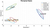 |
Figure 5. The perceptual space of Session 1 for the mechanically-excited panels: the positions of stimuli in the perceptual space with their 95% confidence ellipses. |
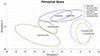 |
Figure 6. The perceptual space of Session 2 for the acoustically-excited panels: the positions of stimuli in the perceptual space with their 95% confidence ellipses. |
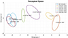 |
Figure 7. The perceptual space of Session 3 for simulations with varied cutoff frequencies: the positions of the stimuli in the perceptual space and their corresponding 95% confidence interval ellipses. |
3.1.1 Session 1: Mechanical excitation
Figure 5 shows the perceptual space for mechanically excited panels. The simulated and recorded stimuli closely align within 95% confidence intervals. The simulations used the modeling approach from [31], validating its effectiveness for composite sandwich panels. Similar agreement was found for composite laminate and steel panels. However, participants struggled to differentiate between laminate and aluminum stimuli, likely due to similar mechanical parameters as shown in Table 1. Despite this, the simulated and recorded stimuli for the laminate panel and aluminum panel remained within their respective confidence ellipses. The authors’ auditory observations, based on qualitative listening to the stimuli, revealed notable patterns that included a transition from loud to soft sounds along Dimension 1 and a shift from treble to bass along Dimension 2, especially between aluminum and composite, and aluminum and steel plates. The number of stimuli was insufficient for a correlation analysis between perceptual dimensions and psychoacoustic indices to statistically validate the auditory assessment.
3.1.2 Session 2: Acoustic excitation
Figure 6 displays alignment between simulated and recorded stimuli for acoustically excited panels. The composite and steel panels have closely positioned stimuli within 95% confidence ellipses. In contrast, the stimuli of aluminum panel were distant, likely due to its greater thickness and the corresponding limitations of the 4th order model used for modeling this isotropic plate. Such a limitation was not observed for the thin steel panel (see Fig. 6). The composite panel was modeled using the 6th order model. Auditory observations, which was based on qualitative listening to the stimuli, were similar to those in the mechanical excitation session, with Dimension 2 showing a bass to treble transition, though less distinct. Larger error ellipsoids (Fig. 6) indicated that participants found it harder to differentiate stimuli compared to the mechanical session (Fig. 5).
Hence, considering the larger error ellipsoids, we observed that stimuli under acoustic excitation showed slightly less separation compared to those under mechanical excitation. This is attributed to the broader excitation of multiple structural modes, which smooths perceptual differences. In contrast, mechanical excitation, being more localized on the panel surface, activates specific modes and leads to greater perceptual differentiation.
3.1.3 Session 3: Cutoff frequency
Figure 7 shows how the maximum frequency (cutoff frequency) affects the perception of simulated sounds. Increasing the cutoff frequency aligns the stimuli with the reference simulation (labeled “Composite (Sim)”) until it reaches 7 kHz. The reference simulation is the simulation with maximum frequency 10 kHz used in Session 1 (labeled “Composite (Sim)”), which closely matches the real recorded stimulus (“Composite (Mic)”) (see Fig. 5). Thus, a cutoff of 7 kHz was chosen for next simulations, supported by the high similarity between the 7 kHz simulation and the reference one within 95% confidence ellipses (see Fig. 7). Furthermore, in Session 3, although the L-Curve method suggested a 2D perceptual space, a 1D space was also explored due to the single parameter (cutoff frequency) being manipulated. The 1D space mirrored Dimension 1 of the 2D space with similar conclusions about stimulus differences within the 95% confidence interval. Dimension 1 appeared related to the transition from treble to bass sounds, as seen when comparing stimuli with cutoff frequencies of 7 kHz and 2 kHz.
3.2 Design and optimization
First, following the classification method described in Section 2.4, AHC was considered to detect potential outliers among participants who participated in the two sessions of the psychoacoustic test for the design optimization. The average linkage method consistently yielded the highest cophenetic and Goodman–Kruskal correlation coefficients [46–48] across both test sessions. Using this method, dendrograms for dissimilarity and preference judgments were obtained in each session. The quality index [49] indicated 2 classes for each dendogram, revealing then the outliers (cf. [80]). In the mechanical session, participants 12 and 31 formed a distinct cluster, while in the acoustic session, participant 12 was identified as an outlier. These results indicate significant response deviations, leading to the exclusion of participants 12 and 31 from the mechanical session and participant 12 from the acoustic session.
3.2.1 Perceptual space
As described in Section 2.4, the INDSCAL algorithm was utilized to analyze the dissimilarity data collected during the two sessions of the psychoacoustic test (see [50–53]). The L-curve method was employed to determine the optimal number of dimensions within the perceptual space. According to the L-curve results, the number of dimensions was 2 for both sessions.
Figures 8 and 9 corresponding to the mechanical and acoustic sessions display the stimuli in the perceptual spaces with 95% confidence intervals (cf. Sect. 3.1).
 |
Figure 8. The perceptual space corresponding to the mechanical excitation. |
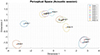 |
Figure 9. The perceptual space corresponding to the acoustic excitation. |
3.2.2 Preference score
Figures 10 and 11 show mean preference scores for mechanical and acoustic sessions, with respective 95% confidence intervals. Design 2 stands out with the highest preference score in the mechanical session, while Designs 7 and 8 excel in the acoustic session. According to Figures 10 and 11, differences in preference ratings are due to the distinct nature of the excitations. The mechanical excitation, being localized, activates specific modes (cf. Fig. 4), leading to tonal contrasts and greater perceptual differences between the sound radiation of some designs (e.g., designs 7 and 8). Comparatively, acoustic excitation, being distributed on the panel surface, excites a broader range of modes, resulting in less tonal contrasts and less perceptual differences between sound radiations of some designs (e.g., no perceptual differences between designs 7 and 8).
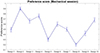 |
Figure 10. The preference scores of the designs in the mechanical excitation. |
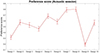 |
Figure 11. The preference scores of the designs in the acoustic excitation. |
3.2.3 Preference and perceptual dimensions
Analyzing data from each test session, a correlation between preference score and a specific dimension in the perceptual space was found. In the mechanical session, a significant correlation was detected between preference and the 2nd dimension (r=0.88,p=0.001). Conversely, in the acoustic session, preference showed a significant correlation with the 1st perceptual dimension (r=0.96,p<0.001).
3.2.4 Impression of stimuli along perceptual dimensions
Based on the authors’ personal listening to the stimuli ranked along each perceptual dimension, variations in key auditory attributes were observed. In the mechanical session, Dimension 1 was associated with a progression from bass sounds to treble sounds. On the other hand, Dimension 2 showed a slight shift from loud to soft sounds. In the acoustic session, Dimension 1 was primarily linked to a shift from loud to soft sounds, while Dimension 2 reflected a transition from bass to treble sounds. Regarding the auditory impression of preference, it was observed that moving from the lowest to the highest of Dimension 2 was primarily associated with the least preferred to the most preferred stimuli in the mechanical session. Similarly, Dimension 1 in the perceptual space of the acoustic session mirrored this preference trend.
3.2.5 Analysis of psychoacoustic indices
In the perceptual space of the mechanical session, Dimension 1 exhibited noteworthy correlations with Sharpness and SC, as indicated by the statistical parameters (r=0.70,p=0.023) and (r=0.78,p=0.008), respectively. Also, the statistical results demonstrated that the preference for the stimuli in the mechanical session exhibited a significant correlation with loudness level, with statistical parameters (r=−0.83,p=0.003). Although a notable correlation was observed between preference and the second perceptual dimension (as shown in Sect. 3.2.3), Dimension 2 did not reach a significant correlation with loudness level in the mechanical session (its statistical parameters for testing the correlation were (r=−0.58,p=0.077) despite the slight shift from loud to soft detected when listening to stimuli along this dimension.
Regarding the acoustic session, Dimension 1 showed a significant correlation with loudness level, with the statistical parameters (r=−0.93,p<0.001). Moreover, Dimension 2 in the acoustic session displayed a significant correlation with Sharpness, supported by the parameters (r=0.81,p=0.005). On the other hand, the statistical results demonstrated that the preference score in the acoustic session exhibited a significant correlation with loudness level, with statistical parameters (r=−0.93,p<0.001). As mentioned in Section 3.2.3, the preference exhibited a significant correlation with the 1st dimension of the perceptual space.
Furthermore, an examination of the relationship between preference and the SPL[dB(A)] was conducted. In the mechanical session, this correlation did not yield statistically significant results, as indicated by the parameters (r=−0.19,p=0.588). This result was expected due to values in dB(A) for stimuli of this session (cf. Tab. 4). The correlation between preference and loudness level was due to the fact that most of the sounds radiated by the vibrating composite panels have got energy at low frequencies. Loudness and loudness level are well-known to be better adapted to account for energy at low frequency (cf. [84]). Conversely, during the acoustic session, unlike the mechanical session, a statistically significant correlation between preference and SPL [dB(A)] was observed, supported by the parameters (r=−0.72,p=0.018), and due to variations in dB(A) observed for stimuli of this session (cf. Tab. 4). However, it is important to note that this correlation was weaker than the significant correlation between preference and loudness level, and mainly explained by the energy content at low frequencies of the stimuli (cf. Fig. 4).
The above-mentioned statistical examination of the correlation between preference and loudness level suggests the possibility of constructing a linear model for predicting the preference. Interestingly, our findings indicated that the coefficients of this model appear to be statistically consistent in each of the two independent sessions involving the mechanical and acoustic excitations. Such a linear model can take the form of the following equation:
 (8)
(8)
Here, LN(s) represents the loudness level in phon according to Zwicker's calculation methods ISO532B and ISO532-1:2017, and P stands for the preference score corresponding to the stimulus s. Tables 5 and 6 display the coefficients derived for the aforementioned model, corresponding to the mechanical and acoustic sessions, respectively. These tables indicate that the coefficients of the model in both sessions are statistically significant. To compare the two models, preference scores for the acoustic and mechanical sessions were cross-predicted. Figures 12 and 13 are displaying the prediction quality of the two preference models. According to these results, using the mechanical preference model for both mechanical and acoustic excitations can be proposed based on these results of cross-validation of the models. When the mechanical preference model was applied to the acoustic session, it demonstrated strong prediction accuracy, with predicted preference scores closely matching the measured ones. Conversely, the acoustic preference model underperformed when applied to the mechanical session, indicating a limited generalization ability. This suggests that the mechanical preference model better captures key perceptual and mechanical factors shared across both types of excitation, making it a more robust option for predicting preference.
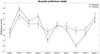 |
Figure 12. Prediction quality of the acoustic preference model: the comparison of the measured preference scores of the mechanical session with the one predicted by the acoustic model presented by Table 6, along with the 95% prediction intervals. |
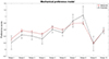 |
Figure 13. Prediction quality of the mechanical preference model: the comparison of the measured preference scores of the acoustic session with the one predicted by the mechanical model presented by Table 5, along with the 95% prediction intervals. |
The statistical results for the regression model P(s)=αLN(s)+α0 between the preference and loudness level for the mechanical session.
The statistical results for the regression model P(s)=αLN(s)+α0 between the preference and loudness level for the acoustic session.
3.2.6 Analysis of mechanical parameters
Analyzing the correlation between design parameters (see Tab. 3), perceptual dimensions, and preference scores presents complexities due to interdependencies and nonlinear relationships among the design parameters. Thus, establishing a regression model between design parameters and perceptual dimensions or preferences is challenging. However, regression analysis can identify key design parameters influencing both preferences and perceptual dimensions, aiding future composite panel design optimization. The correlation analysis carried out for both session data highlighted that the stiffness-to-mass ratio (Dt/M) showed the strongest correlation with the first perceptual dimension in both mechanical and acoustic sessions, as well as the preference score in the acoustic session ((r=0.85,p=0.002), (r=0.90,p<0.001), (r=0.85,p=0.002), respectively).
According to the psychoacoustic analysis in Section 3.2.5, for the mechanical session, Dimension 1 correlates with sharpness, while in the acoustic session, it relates to loudness. The stiffness-to-mass ratio, defined as the ratio of bending stiffness D to surface mass density M, directly affects both amplitude and natural frequency of the vibroacoustic response (cf. [31, 32]). This parameter influences quantities related to amplitude and energy, such as sound pressure and loudness levels. Additionally, since the stiffness-to-mass ratio affects natural frequencies, its variation can shift these frequencies and alter psychoacoustic indices like spectral centroid (SC) and sharpness, which depend on energy distribution across frequencies. Analyzing both sessions shows that the mechanical excitation, Dimension 1 (connected to the stiffness-to-mass ratio) links to sharpness and SC, while in the acoustic excitation, it links to loudness and sound pressure level (SPL). This is because acoustic excitation affects all natural modes by applying to the entire vibrating panel surface, allowing stiffness-to-mass ratio variations to impact more natural frequencies, thus influencing loudness and SPL more significantly than point-wise mechanical excitation.
As a result, an investigation into the regression-based statistical analyses between several physical parameters and preference scores was also carried out, in order to find a model of mechanical parameters for calculating the preference scores. A suitable linear regression model was identified for the acoustic session, while for the mechanical session, no acceptable linear regression model could be established. This led us to suspect the presence of nonlinear terms in the model. Subsequently, various nonlinear regression models, including terms with a power of 2, were explored for the mechanical session. The selection of the most appropriate model for both sessions was based on the highest adjusted coefficient of determination R2, and ensured independence and physical meaningfulness between the chosen parameters.
Tables 7 and 8 provide the regression models with the respective significant coefficients. The regression analyses in the both sessions showed that the preference scores depend on the same mechanical parameters: stiffness-to-mass ratio Dt/M and loss damping factors η (cf. Tabs. 7 and 8).
The regression model for preference P in the mechanical session in relation to the mechanical parameters η, and Dt/M, where r is the correlation between the modeled and measured preference, and the model is defined as P=α0+α1η+α2Dt/M+α3(Dt/M)2.
The regression model for preference P in the acoustic session in relation to the mechanical parameters η, and Dt/M, where r is the correlation between the modeled and measured preference, the regression model is defined as P=α0+α1η+α2Dt/M.
Furthermore, to independently evaluate the correlation between preferences and each of these parameters (the stiffness-to-mass ratio Dt/M and loss damping factors η), partial correlation analyses were conducted. For the session with mechanical excitation, the partial correlation between the loss damping factor η and the preference score was calculated, while controlling for the effects of Dt/M and the nonlinear term (Dt/M)2. The estimated partial correlation of η with the preference and the corresponding p-value was (r=0.86,p=0.006). Similarly, a partial correlation between the stiffness-to-mass ratio Dt/M and the preference score was performed, while controlling for the effects of η and the nonlinear term (Dt/M)2, yielding the result (r=0.89,p=0.002). Likewise, for the session with acoustic excitation, the partial correlation analyses were conducted to obtain the partial correlations of Dt/M and η with preferences. This was done while controlling for the effect of one parameter on the correlation of the other. The partial correlations of η and Dt/M were obtained equal to (r=−0.80,p=0.009) and (r=0.95,p<0.001), respectively. In all these results, the partial correlations were significant. They confirm the relevance of the obtained regression models. Notably, the partial correlation between the stiffness-to-mass ratio Dt/M and preference for the acoustic session showed an increase compared to the value of the ordinary correlation mentioned before.
3.3 Optimal designs
Due to the distinct physical nature of mechanical and acoustic excitations, uncorrelated preferences between the two sessions were anticipated. Statistical analysis confirmed this lack of correlation (r=−0.22,p=0.548). Visualization of the Pareto front has proven effective in identifying optimal solutions for independent objectives (e.g., see [85]). Therefore, optimal designs were pursued considering mechanical and acoustic preferences as two separate objectives. Figure 14 shows the 10 designs tested in the psychoacoustic assessment, highlighting Designs 2, 6, 7, and 8 as the optimal non-dominated solutions on the Pareto Front. These designs consistently achieved higher preference scores in both sessions. Upon closer examination of the Pareto Front (Designs 2, 6, 7, and 8) using their 95% confidence intervals (cf. Fig. 14), Designs 2 and 6 show no significant difference in the acoustic session, but Design 2 outperforms Design 6 in the mechanical session. Similarly, while Designs 7 and 8 show no significant difference in the acoustic session, Design 7 surpasses Design 8 in the mechanical session. Thus, the Pareto Front identifies Designs 2 and 7 as the most optimal choices among the other ones. Indeed, these two designs have different mechanical parameters, and to determine the most suitable choice, their mechanical properties should be emphasized. Referring to Table 3, Design 7 exhibits a superior stiffness-to-mass ratio, and in certain applications such as aircraft or robotic structure design, this ratio holds critical significance when selecting materials for structural components (e.g., see [86–89]). However, Design 2 is lighter than Design 7 (see Tab. 3). Furthermore, it is worth noting that what makes these Pareto solutions, namely Designs 2 and 7, particularly noteworthy is how they vary depending on the characteristics of the face sheets during the design phase. Design 2 aimed to be linked to the influence of Young's modulus of the face sheets Ef, while Design 7 aimed to be linked to the effect of face sheet thickness hf, where Designs 2 and 7 have the highest values of Ef and hf, respectively. These Pareto results underscore the substantial impact of face sheet characteristics in composite sandwich panel design (cf. Tab. 3 and Fig. 14).
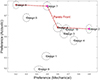 |
Figure 14. The Pareto Front: the graph shows the Pareto optimal solutions (on the red dash-dot line) in 2D, illustrating the preference scores for mechanical and acoustic sessions, displaying the preference scores of 10 designs and their 95% confidence intervals. |
4 Conclusion and discussion
This research makes two key contributions: first, perceptual validation of vibroacoustic modeling for composite panels, and second, optimization of composite sandwich design from an auditory perspective. Essential psychoacoustic processes for accurate panel modeling and simulations (i.e., sound synthesis) were introduced, and simulations were validated through psychoacoustic analyses. For this purpose, three psychoacoustic test sessions in the perceptual validation step, focused on mechanical excitation, acoustic excitation, and optimizing simulation maximum frequency, used pairwise comparisons to measure dissimilarities between recorded and simulated stimuli. Then the INDSCAL multidimensional scaling algorithm was used to analyze the perceptual dissimilarities between the synthesized sounds and laboratory-recorded sounds, and thereby to perceptually validate the vibroacoustic models [31] used for sound synthesis. The third session optimized computational efficiency, recommending 7kHz as the maximum perceptually relevant frequency, supporting prior research (see [28, 90, 91]) on balancing computational cost with perceptual fidelity.
Following the validation of the vibroacoustic models from a psychoacoustic perspective, the research focused on perception-based design and optimization of vibrating composite panels. Using the validated model, various designs were simulated for both mechanical and acoustic excitations, resulting in two psychoacoustic test sessions. Participants provided judgments on dissimilarity and preference. Perceptual spaces were created using the INDSCAL algorithm. The preference scores were correlated to the perceptual dimensions. Correlation analyses showed how psychoacoustic indices influenced preferences, particularly loudness, which had the strongest effect despite minor SPL[dB(A)] differences. This is attributed to the low-frequency energy in the panel sound, where loudness better captures the effect [84]. A linear model predicting preference based on loudness level was developed, offering insights for future composite panel studies.
Statistical analyses were conducted between mechanical parameters, perceptual dimensions, and preference scores. The results revealed that the stiffness-to-mass ratio and loss damping factor were the most influential mechanical parameters for all excitation types. Two regression models were also introduced, linking preference to these key mechanical parameters. Previous studies have explored this relationship. For example, Faure and Marquis-Favre [24] found a strong correlation between preference and mechanical properties of an isotropic plate, particularly its thickness and damping. Similarly, Miloudi et al. [92] showed the impact of thickness and damping on radiated noise and sound perception. These findings as well as the current study highlight how structural parameters such as stiffness-to-mass ratio and loss damping factor can be tuned to influence perceived sound quality – a valuable insight for vibroacoustic engineers aiming to optimize both mechanical and perceptual performances.
Using the Pareto Front visualization, optimal designs were identified considering the two types of excitations. The Pareto solutions emphasized that the Young's modulus and face sheet thickness are critical for optimal composite panel design. Similar effects of these parameters on perceptual dimensions and sound preference have been observed for isotropic panels (e.g., [24]). Theoretically, the face sheet parameters Ef and hf are tied to the stiffness-to-mass ratio Dt/M, which impacts the preference score. Additionally, the stiffness-to-mass ratio affects loudness level and sharpness, varying with excitation type. Such influences of mechanical parameters on multiple psychoacoustic indices determining sound quality have been studied in other works (e.g., [16]).
In this study, psychoacoustic metrics such as loudness level, as well as mechanical parameters like stiffness-to-mass ratio and damping factor, were separately examined in relation to the preference ratings gathered during the listening test sessions. This dual approach enabled us to qualitatively link perceptual trends with both structural design variables and psychoacoustic indices. Future works may focus on developing direct quantitative models that explicitly relate physical properties to psychoacoustic indices. Future studies integrating vibroacoustic modeling with psychoacoustic assessment could be conducted to account for a wider range of mechanical and geometrical parameters. The rationale and approaches proposed in this work may be utilized to achieve optimal designs. Additionally, the state-of-the-art techniques like Artificial Intelligence and Deep Learning methods could be explored for design optimization, incorporating perceptual perspectives.
In addition to loudness level, the base-10 logarithm of loudness was also analyzed, yielding similar conclusions to the ones obtained with loudness level.
Acknowledgments
Also, the authors would like to express their thanks to Prof. Etienne PARIZET for sharing his INDSCAl algorithm. We sincerely thank the editor, reviewers, and examiners of this work for devoting their valuable time to enhancing our research.
Funding
Financial supports of the Centre Lyonnais d’Acoustique, CeLyA (Lyon Acoustics Center, ANR-10-LABX-0060), are gratefully acknowledged.
Conflicts of interest
The authors declare that they have no known competing financial interests or personal relationships that could have appeared to influence the work reported in this paper.
Data availability statement
Data are available on request from the authors.
Author contribution statement
Y. AllahTavakoli: Conceptualization, Methodology, Laboratory experiments, Simulations, Software, Validation, Investigation, Writing – original draft. C. Marquis-Favre: Conceptualization, Supervision, Methodology, Validation, Investigation, Writing – review and editing. M.N. Ichchou: Conceptualization, Supervision, Validation, Investigation, Writing – review and editing. N. Hamzaoui: Conceptualization, Supervision, Methodology, Validation, Investigation, Writing – review and editing.
References
- V. Giurgiutiu: Structural Health Monitoring of Aerospace Composites. Academic Press, Oxford, 2015, pp. 1–23 [Google Scholar]
- J. Fan, J. Njuguna: An introduction to lightweight composite materials and their use in transport structures, in: Lightweight Composite Structures in Transport. Elsevier, 2016, pp. 3–34 [Google Scholar]
- R.F. Gibson: Principles of Composite Material Mechanics. CRC Press, 2016 [Google Scholar]
- J.-M. Berthelot, F.F. Ling: Composite Materials: Mechanical Behavior and Structural Analysis. Vol. 435. Springer, 1999 [Google Scholar]
- D.J. Mead, S. Markus: The forced vibration of a three-layer, damped sandwich beam with arbitrary boundary conditions. Journal of Sound and Vibration 10, 2 (1969) 163–175 [Google Scholar]
- A.W. Christian, R. Cabell: Initial investigation into the psychoacoustic properties of small unmanned aerial system noise, in: 23rd AIAA/CEAS Aeroacoustics Conference, 2017, p. 4051 [Google Scholar]
- C.T. Justine Hui, M.J. Kingan, Y. Hioka, G. Schmid, G. Dodd, K.N. Dirks, S. Edlin, S. Mascarenhas, Y.-M. Shim, Quantification of the psychoacoustic effect of noise from small unmanned aerial vehicles. International Journal of Environmental Research and Public Health 18, 17 (2021) 8893 [Google Scholar]
- A.J. Torija, Z. Li, P. Chaitanya: Psychoacoustic modelling of rotor noise. The Journal of the Acoustical Society of America 151, 3 (2022) 1804–1815 [CrossRef] [PubMed] [Google Scholar]
- F.D. Monteiro, R. Merino-Martinez, L.T. Lima Pereira: Psychoacoustic evaluation of an array of distributed propellers under synchrophasing operation, in: 30th AIAA/CEAS Aeroacoustics Conference, 2024, p. 3321 [Google Scholar]
- E. Parizet, E. Guyader, V. Nosulenko: Analysis of car door closing sound quality. Applied Acoustics 69, 1 (2008) 12–22 [Google Scholar]
- H.B. Huang, X.R. Huang, R.X. Li, T.C. Lim, W.P. Ding: Sound quality prediction of vehicle interior noise using deep belief networks. Applied Acoustics 113 (2016) 149–161 [Google Scholar]
- U. Letens, A. Oetjen, D. Goecke, D. Maiberger: Practical Experience with Psychoacoustics in Automotive Engineering. Universitätsbibliothek der RWTH Aachen, 2019 [Google Scholar]
- Z. Ouelaa, R. Younes, A. Djebala, N. Hamzaoui, N. Ouelaa: Comparative study between objective and subjective methods for identifying the gravity of single and multiple gear defects in case of noisy signals. Applied Acoustics 185 (2022) 108432 [Google Scholar]
- X. Chen, J. Lin, H. Jin, Y. Huang, Z. Liu: The psychoacoustics annoyance research based on eeg rhythms for passengers in high-speed railway. Applied Acoustics 171 (2021) 107575 [CrossRef] [Google Scholar]
- J. Theyssen: The radiation from railway wheel modes and their effect on loudness, sharpness, and equivalent pressure level. Acta Acustica 8 (2024) 20 [Google Scholar]
- S. Atamer, M.E. Altinsoy: Sound quality of dishwashers: annoyance perception. Applied Acoustics 180 (2021) 108099 [Google Scholar]
- J. Tardieu, P. Susini, F. Poisson, P. Lazareff, S. McAdams: Perceptual study of soundscapes in train stations. Applied Acoustics 69, 12 (2008) 1224–1239 [Google Scholar]
- G. Fusaro, J. Kang, F. Asdrubali, W.-S. Chang: Assessment of acoustic metawindow unit through psychoacoustic analysis and human perception. Applied Acoustics 196 (2022) 108885 [Google Scholar]
- M.G. Roest: Design of a composite guitar. Master thesis report, Delft University of Technology (TU Delft), 2016 [Google Scholar]
- T. Duerinck, G. Verberkmoes, C. Fritz, M. Leman, L. Nijs, M. Kersemans, W. Van Paepegem: Listener evaluations of violins made from composites. The Journal of the Acoustical Society of America 147, 4 (2020) 2647–2655 [Google Scholar]
- S. Meunier, D. Habault, G. Canévet: Auditory evaluation of sound signals radiated by a vibrating surface. Journal of Sound and Vibration 247, 5 (2001) 897–915 [Google Scholar]
- G. Canévet, D. Habault, S. Meunier, F. Demirdjian: Auditory perception of sounds radiated by a fluid-loaded vibrating plate excited by a transient point force. Acta Acustica united with Acustica 90, 1 (2004) 181–193 [Google Scholar]
- F. Demirdjian, D. Habault, S. Meunier, G. Canévet: Can we hear the complexity of vibrating plates, in: Proceedings of the CFADAGA Conference, 2004 [Google Scholar]
- J. Faure, C. Marquis-Favre: Perceptual assessment of the influence of structural parameters for a radiating plate. Acta Acustica united with Acustica 91, 1 (2005) 77–90 [Google Scholar]
- F. Demirdjian, S. Meunier, D. Habault, G. Canévet: A comparative study of recorded and computed sounds radiated by vibrating plates, in: Proc. of Forum Acusticum, 2005 [Google Scholar]
- C. Marquis-Favre, J. Faure: Auditory evaluation of sounds radiated from a vibrating plate with various viscoelastic boundary conditions. Acta Acustica united with Acustica 94, 3 (2008) 419–432 [Google Scholar]
- A. Trollé, C. Marquis-Favre, J. Faure: An analysis of the effects of structural parameter variations on the auditory perception of environmental noises transmitted through a simulated window. Applied Acoustics 69, 12 (2008) 1212–1223 [Google Scholar]
- A. Trollé, C. Marquis-Favre, N. Hamzaoui: Auditory evaluation of sounds radiated from a vibrating plate inside a damped cavity. Acta Acustica united with Acustica 95, 2 (2009) 343–355 [Google Scholar]
- S. McAdams, V. Roussarie, A. Chaigne, B.L. Giordano: The psychomechanics of simulated sound sources: material properties of impacted thin plates. The Journal of the Acoustical Society of America 128, 3 (2010) 1401–1413 [Google Scholar]
- J. Hjortkjær, S. McAdams: Spectral and temporal cues for perception of material and action categories in impacted sound sources. The Journal of the Acoustical Society of America 140, 1 (2016) 409–420 [Google Scholar]
- Y. AllahTavakoli, M.N. Ichchou, C. Marquis-Favre, N. Hamzaoui: On a hybrid updating method for modeling vibroacoustic behaviors of composite panels. Journal of Sound and Vibration 565 (2023) 117902 [Google Scholar]
- Y. AllahTavakoli, C. Marquis-Favre, M. Ichchou, N. Hamzaoui: On the vibro-acoustic modeling of panels excited by diffuse acoustic field (DAF), in: INTER-NOISE and NOISE-CON Congress and Conference Proceedings. Vol. 265. Institute of Noise Control Engineering, 2023, pp. 4354–4365 [Google Scholar]
- E. Ventsel, T. Krauthammer, E. Carrera: Thin plates and shells: theory, analysis, and applications. Applied Mechanics Reviews 55, 4 (2002) B72–B73 [Google Scholar]
- K. Kohsaka, K. Ushijima, W.J. Cantwell: Study on vibration characteristics of sandwich beam with BCC lattice core. Materials Science and Engineering: B 264 (2021) 114986 [Google Scholar]
- S. Narayanan, R.L. Shanbhag: Sound transmission through a damped sandwich panel. Journal of Sound and Vibration 80, 3 (1982) 315–327 [Google Scholar]
- F.J. Fahy: Foundations of Engineering Acoustics. Elsevier, 2000 [Google Scholar]
- S. Narayanan, R.L. Shanbhag: Sound transmission through elastically supported sandwich panels into a rectangular enclosure. Journal of Sound Vibration 77, 2 (1981) 251–270 [Google Scholar]
- C. Marchetto, L. Maxit, O. Robin, A. Berry: Vibroacoustic response of panels under diffuse acoustic field excitation from sensitivity functions and reciprocity principles. The Journal of the Acoustical Society of America 141, 6 (2017) 4508–4521 [Google Scholar]
- W.L. Briggs, V.E. Henson: The DFT: an owner's Manual for the Discrete Fourier Transform. SIAM, 1995 [Google Scholar]
- V. Koehl, E. Parizet: Influence of structural variability upon sound perception: usefulness of fractional factorial designs. Applied Acoustics 67, 3 (2006) 249–270 [Google Scholar]
- J. Faure: Influence des paramètres structuraux d’une plaque rayonnante sur la perception sonore. PhD thesis, Lyon, INSA, 2003 [Google Scholar]
- A. Trollé: Evaluation auditive de sons rayonnés par une plaque vibrante à l’intérieur d’une cavité amortie: ajustement des efforts de calcul vibro-acoustique. PhD thesis, INSA de Lyon, 2009 [Google Scholar]
- P. Chevret, E. Parizet: An efficient alternative to the paired comparison method for the subjective evaluation of a large set of sounds, in: Proceedings of the 19th International Congress on Acoustics (ICA 2007). Madrid, 2007, pp. 1–5 [Google Scholar]
- E. Parizet, V. Koehl: Application of free sorting tasks to sound quality experiments. Applied Acoustics 73, 1 (2012) 61–65 [Google Scholar]
- P.-Y. Michaud, S. Meunier, P. Herzog, M. Lavandier, G.D. d’Aubigny: Perceptual evaluation of dissimilarity between auditory stimuli: an alternative to the paired comparison. Acta Acustica united with Acustica 99, 5 (2013) 806–815 [Google Scholar]
- R.R. Sokal, F.J. Rohlf: The comparison of dendrograms by objective methods. Taxon 11 (1962) 33–40 [Google Scholar]
- J.S. Farris: On the cophenetic correlation coefficient. Systematic Zoology 18, 3 (1969) 279–285 [Google Scholar]
- L.A. Goodman, W.H. Kruskal, L.A. Goodman, W.H. Kruskal: Measures of Association for Cross Classifications. Springer, 1979 [Google Scholar]
- J.-P. Nakache, J. Confais: Approche pragmatique de la classification: arbres hiérarchiques, partitionnements. Editions Technip, 2004 [Google Scholar]
- J.D. Carroll, J.-J. Chang: Analysis of individual differences in multidimensional scaling via an n-way generalization of eckart-young decomposition. Psychometrika 35, 3 (1970) 283–319 [Google Scholar]
- J.D. Carroll: Individual differences and multidimensional scaling. Multidimensional Scaling: Theory and Applications in the Behavioral Sciences 1 (1972) 105–155 [Google Scholar]
- J.D. Carroll, P. Arabie: Multidimensional scaling. Measurement, Judgment and Decision Making (1998) 179–250 [Google Scholar]
- I. Borg, P.J.F. Groenen: Modern Multidimensional Scaling: Theory and Applications. Springer Science & Business Media, 2005 [Google Scholar]
- N. Jaworska, A. Chupetlovska-Anastasova: A review of multidimensional scaling (MDS) and its utility in various psychological domains. Tutorials in Quantitative Methods for Psychology 5, 1 (2009) 1–10 [Google Scholar]
- M.C. Hout, M.H. Papesh, S.D. Goldinger: Multidimensional scaling. Wiley Interdisciplinary Reviews: Cognitive Science 4, 1 (2013) 93–103 [Google Scholar]
- P.C. Hansen: The L-curve and its use in the numerical treatment of inverse problems, in: Computational Inverse Problems in Electrocardiology Conference, 1999 [Google Scholar]
- F. Ponsi, E. Bassoli, L. Vincenzi: A multi-objective optimization approach for fe model updating based on a selection criterion of the preferred pareto-optimal solution, in: Structures. Vol. 33. Elsevier, 2021, pp. 916–934 [Google Scholar]
- S.L. Weinberg, J.D. Carroll, H.S. Cohen: Confidence regions for indscal using the Jackknife and Bootstrap techniques. Psychometrika 49 (1984) 475–491 [Google Scholar]
- S. Ghinet, N. Atalla: Modeling thick composite laminate and sandwich structures with linear viscoelastic damping. Computers & Structures 89, 15, 16 (2011) 1547–1561 [Google Scholar]
- J. Li, Y. Narita: Analysis and optimal design for the damping property of laminated viscoelastic plates under general edge conditions. Composites Part B: Engineering 45, 1 (2013) 972–980 [Google Scholar]
- D. Montalvão, R. Cláudio, A.M.R. Ribeiro, J. Duarte-Silva: Experimental measurement of the complex young's modulus on a CFRP laminate considering the constant hysteretic damping model. Composite Structures 97 (2013) 91–98 [Google Scholar]
- R. Cherif, J.-D. Chazot, N. Atalla: Damping loss factor estimation of two-dimensional orthotropic structures from a displacement field measurement. Journal of Sound and Vibration 356 (2015) 61–71 [Google Scholar]
- E. Sarlin, Y. Liu, M. Vippola, M. Zogg, P. Ermanni, J. Vuorinen, T. Lepistö: Vibration damping properties of steel/rubber/composite hybrid structures. Composite Structures 94, 11 (2012) 3327–3335 [Google Scholar]
- Z. Zergoune, M.N. Ichchou, O. Bareille, B. Harras, R. Benamar, B. Troclet: Assessments of shear core effects on sound transmission loss through sandwich panels using a two-scale approach. Computers & Structures 182 (2017) 227–237 [Google Scholar]
- Z. Qi, Y. Liu, W. Chen: An approach to predict the mechanical properties of CFRP based on cross-scale simulation. Composite Structures 210 (2019) 339–347 [Google Scholar]
- Y. Zhou, A. Liu, Y. Xu, Y. Guo, X. Yi, Y. Jia: Frequency-dependent orthotropic damping properties of nomex honeycomb composites. Thin-Walled Structures 160 (2021) 107372 [Google Scholar]
- M.N. Collins, M. Culebras, G. Ren: Chapter 8 – the use of lignin as a precursor for carbon fiber-reinforced composites, in: D. Puglia, C. Santulli, F. Sarasini, Eds. Micro and Nanolignin in Aqueous Dispersions and Polymers. Elsevier, 2022, pp. 237–250 [Google Scholar]
- L.L. Thurstone: A law of comparative judgment. Psychological Review 34, 4 (1927) 273 [Google Scholar]
- T. Bramley: Paired comparison methods. Techniques for Monitoring the Comparability of Examination Standards 246 (2007) 294 [Google Scholar]
- T.J. DiCiccio, B. Efron: Bootstrap confidence intervals. Statistical Science 11, 3 (1996) 189–228 [Google Scholar]
- E. Zwicker, H. Fastl, U. Widmann, K. Kurakata, S. Kuwano, S. Namba: Program for calculating loudness according to DIN 45631 (ISO 532B). Journal of the Acoustical Society of Japan (E) 12, 1 (1991) 39–42 [Google Scholar]
- dBsonic Manual: dbsonic sound analysis software. Software manual, 2005 [Google Scholar]
- Q. Legros: Caractérisation physique et perceptive des bruits de passage de TGV pour une amélioration des modèles de gêne. Master thesis report, ENTPE, 2020 [Google Scholar]
- ISO: Acoustics – methods for calculating loudness – part 1: Zwicker method, 2017 [Google Scholar]
- W. Aures: Berechnungsverfahren für den sensorischen wohlklang beliebiger schallsignale. Acta Acustica united with Acustica 59, 2 (1985) 130–141 [Google Scholar]
- W. Aures: Ein berechnungsverfahren der rauhigkeit. Acta Acustica united with Acustica 58, 5 (1985) 268–281 [Google Scholar]
- M.S. Engel, A. Fiebig, C. Pfaffenbach, J. Fels: A review of the use of psychoacoustic indicators on soundscape studies. Current Pollution Reports 7 (2021) 359–378 [CrossRef] [Google Scholar]
- J. Branke: Multiobjective Optimization: Interactive and Evolutionary Approaches. Vol. 5252. Springer Science & Business Media, 2008 [Google Scholar]
- K. Deb: Multi-objective optimisation using evolutionary algorithms: an introduction, in: Multi-objective Evolutionary Optimisation for Product Design and Manufacturing. Springer, 2011, 3–34 [Google Scholar]
- Y. AllahTavakoli: A contribution to the vibroacoustic and psychoacoustic design of composite structures. Theses, École Nationale des Travaux Publics de l’État [ENTPE], https://theses.hal.science/tel-04659121v1/file/Allah_Tavakoli_PhD_thesis_2023.pdf, December 2023 [Google Scholar]
- P.C. Hansen: regtools: regularization tools, 2023 [Google Scholar]
- P.C. Hansen: Regularization tools version 4.0 for matlab 7.3. Numerical Algorithms 46 (2007) 189–194 [Google Scholar]
- R.A. Johnson, D.W. Wichern: Applied Multivariate Statistical Analysis. Prentice Hall, 2002 [Google Scholar]
- E. Zwicker, H. Fastl: Psychoacoustics: Facts and Models. Vol. 22. Springer Science & Business Media, 2013 [Google Scholar]
- R.T. Marler, J.S. Arora: Survey of multi-objective optimization methods for engineering. Structural and Multidisciplinary Optimization 26 (2004) 369–395 [CrossRef] [MathSciNet] [Google Scholar]
- C.M. Shearer, C.E.S. Cesnik: Nonlinear flight dynamics of very flexible aircraft. Journal of Aircraft 44, 5 (2007) 1528–1545 [Google Scholar]
- B.J. Kim, D.K. Yun, S.H. Lee, G.-W. Jang: Topology optimization of industrial robots for system-level stiffness maximization by using part-level metamodels. Structural and Multidisciplinary Optimization 54 (2016) 1061–1071 [Google Scholar]
- B.T. Warwick, C.K. Mechefske, I.Y. Kim: Topology optimization of a pre-stiffened aircraft bulkhead. Structural and Multidisciplinary Optimization 60 (2019) 1667–1685 [Google Scholar]
- F.A. Pires, M. Wandel, C. Thomas, E. Deckers, W. Desmet, C. Claeys: Improving the sound transmission loss of an aircraft ceiling panel by locally resonant metamaterials. Technical report, SAE Technical Paper, 2022 [Google Scholar]
- A. Trolle, C. Marquis-Favre, N. Hamzaoui: Auditory evaluation of sounds radiated from a vibrating plate inside a damped cavity: adjustment of the frequency resolution of vibro-acoustical computing. Acta Acustica united with Acustica 98, 3 (2012) 441–450 [Google Scholar]
- G. Pulvirenti, N. Totaro, E. Parizet: A perceptual evaluation of numerical errors in acoustic FEM simulation for sound quality applications. Applied Acoustics 207 (2023) 109295 [Google Scholar]
- A. Miloudi, N. Hamzaoui, J.-L. Guyader: Subjective evaluations of sound radiated by impacted plates, using the design of experiments method. Applied Acoustics 71, 6 (2010) 531–538 [Google Scholar]
Cite this article as: AllahTavakoli Y. Marquis-Favre C. Ichchou M.N. & Hamzaoui N. 2025. A psychoacoustic assessment for enhancing the sound quality of vibrating composite panels. Acta Acustica, 9, 48. https://doi.org/10.1051/aacus/2025031.
All Tables
The properties of stimuli: dimensions a×b, thickness h, bending stiffness D, Young's modulus E, Poisson ratio ν, surface mass density M, and loss damping factor η of vibrating panels. fM: cutoff frequency for simulation, SPL: mean A-weighted sound pressure level. “S.”, “No.”, and “Exc.” denote session, stimulus number, and excitation type. “Mech” and “Acous” refer to mechanical and acoustic excitations; “Mic” and “Sim” to microphone-recorded or simulated stimuli.
The composite sandwich panel parameters, tested in vibroacoustic experiments by AllahTavakoli et al. [31]: dimensions a×b, face sheet thickness hf, core thickness hc, and Dt, Ef, G, ν, and η represent the total bending stiffness, Young's modulus of face sheets, core shear modulus, Poisson ratio, and loss damping factor, respectively.
The sound pressure levels of the stimuli for the designed composite panels excited by the mechanical and acoustic excitations, [unit: dB(A)].
The statistical results for the regression model P(s)=αLN(s)+α0 between the preference and loudness level for the mechanical session.
The statistical results for the regression model P(s)=αLN(s)+α0 between the preference and loudness level for the acoustic session.
The regression model for preference P in the mechanical session in relation to the mechanical parameters η, and Dt/M, where r is the correlation between the modeled and measured preference, and the model is defined as P=α0+α1η+α2Dt/M+α3(Dt/M)2.
The regression model for preference P in the acoustic session in relation to the mechanical parameters η, and Dt/M, where r is the correlation between the modeled and measured preference, the regression model is defined as P=α0+α1η+α2Dt/M.
All Figures
|
Figure 1. The thick composite sandwich panel with a Nomex-honeycomb core and CFRP face sheets, studied by AllahTavakoli et al. [31], from which the designs of the composite panel in the current research was inspired. |
| In the text | |
|
Figure 2. Overview of the steps of the psychoacoustic framework developed for enhancing the sound quality of vibrating composite panels. |
| In the text | |
|
Figure 3. The set-up diagram of (a) the mechanical excitation experiment with a laser vibrometer, spectrum analyzer, signal generator, microphone, and shaker (see [31]), and (b) the diffuse acoustic excitation experiment with an acoustic cabin, four speakers, a 4-microphone array inside the cabin, and a microphone outside (see [32]). |
| In the text | |
|
Figure 4. The SPL spectra for stimuli 8 and 9, corresponding to designs with the highest and lowest values of total bending stiffness Dt, respectively, under mechanical (labeled as “Mech”) and acoustic (labeled as “Acous”) excitations. |
| In the text | |
|
Figure 5. The perceptual space of Session 1 for the mechanically-excited panels: the positions of stimuli in the perceptual space with their 95% confidence ellipses. |
| In the text | |
|
Figure 6. The perceptual space of Session 2 for the acoustically-excited panels: the positions of stimuli in the perceptual space with their 95% confidence ellipses. |
| In the text | |
|
Figure 7. The perceptual space of Session 3 for simulations with varied cutoff frequencies: the positions of the stimuli in the perceptual space and their corresponding 95% confidence interval ellipses. |
| In the text | |
|
Figure 8. The perceptual space corresponding to the mechanical excitation. |
| In the text | |
|
Figure 9. The perceptual space corresponding to the acoustic excitation. |
| In the text | |
|
Figure 10. The preference scores of the designs in the mechanical excitation. |
| In the text | |
|
Figure 11. The preference scores of the designs in the acoustic excitation. |
| In the text | |
|
Figure 12. Prediction quality of the acoustic preference model: the comparison of the measured preference scores of the mechanical session with the one predicted by the acoustic model presented by Table 6, along with the 95% prediction intervals. |
| In the text | |
|
Figure 13. Prediction quality of the mechanical preference model: the comparison of the measured preference scores of the acoustic session with the one predicted by the mechanical model presented by Table 5, along with the 95% prediction intervals. |
| In the text | |
|
Figure 14. The Pareto Front: the graph shows the Pareto optimal solutions (on the red dash-dot line) in 2D, illustrating the preference scores for mechanical and acoustic sessions, displaying the preference scores of 10 designs and their 95% confidence intervals. |
| In the text | |
Current usage metrics show cumulative count of Article Views (full-text article views including HTML views, PDF and ePub downloads, according to the available data) and Abstracts Views on Vision4Press platform.
Data correspond to usage on the plateform after 2015. The current usage metrics is available 48-96 hours after online publication and is updated daily on week days.
Initial download of the metrics may take a while.