© The Author(s), published by EDP Sciences, 2022

1 Introduction

The acoustic comfort in modern product development has significantly gained importance in recent times. Especially in the high-end passenger transportation sector, acoustics plays a major role [1–4]. The current trend to e-mobility further contributes to the importance of acoustic design. Noise arising from auxiliary aggregates can become unpleasant due to the absence of combustion engine noise [5–9]. Ideally, acoustic aspects are already considered during the design phase by means of CAA. When aeroacoustic effects are involved, the hybrid approach is an efficient way to limit the computational effort and to overcome the challenge of the disparity of scales in CAA [10, 11]. The application of this two-step approach to various kinds of flow configurations, such as fans [12, 13], jets [14], and other external flows [15–17] can be found in literature. Aeroacoustics of internal (ducted) flows with constrictions was numerically [18–28] and experimentally [29–32] investigated in the past, considering mostly rectangular ducts with symmetric constrictions. Numerical investigations of a duct flow using Lighthill’s wave equation, solved by FEM, are presented in [18, 19]. The simulations were performed in the frequency domain after Fourier transformation of the acoustic source terms, where a rather small frequency range of 300 Hz ≤ f ≤ 3500 Hz was considered for evaluation. Piellard and Bailly investigated a low Mach number flow through a rectangular duct with a diaphragm, and focused on the impact of the scheme employed for source term interpolation [22, 33]. The acoustic field obtained from a fully compressible Direct Numerical Simulation (DNS) published in [34] was used as a reference.

In the present work, three aeroacoustic formulations based on the hybrid approach, namely Lighthill’s acoustic wave equation, the perturbed convective wave equation, and the dilatation equation of Ribner are applied. In the following the abbreviations LH, PCWE and RIB will be used, respectively. Compared to other aeroacoustic formulations, such as the Linearized Euler Equations (LEE), the selected equations solve only a scalar wave equation and are therefore efficient with regards to the computational effort. However, they differ in the solution quantity (purely acoustic or a superposition with the aerodynamic pressure) and in the source term computation (containing spatial and temporal derivatives). The aim of the present investigations is to determine their suitability for the application in the hybrid approach, especially for duct flows. The variational form of the equations is solved using FEM. The capability of the considered aeroacoustic formulations is demonstrated for low Mach number flows through a half-moon-shaped orifice in a circular pipe. The asymmetric obstruction was chosen to determine the location of the reattachment zone avoiding the possible occurrence of a pitchfork bifurcation [35–37] in order to efficiently position pressure probes in the validation experiment. The governing equations are provided in Section 2, and in Section 3 the workflow is illustrated. The numerical setups of the incompressible Large Eddy Simulation (LES) and the time-domain Computational Acoustic (CA) simulation are presented. Dedicated measurements at three different flow speeds with Mach numbers 0.011, 0.0236, and 0.06 were performed and serve as validation data for the simulations. Furthermore, an extensive analysis of the sound generation mechanisms based on the flow results and an analysis of the acoustic source terms is provided. The contribution of the subgrid-scale (SGS) model to the Lighthill source term and the contribution of the time derivative and convective term to the full PCWE source term are assessed. Contours of the instantaneous acoustic sources are illustrated and spectra at selected locations are discussed. In Section 4, the practical aspects regarding the numerical effort are addressed. Finally, the conclusions are drawn in Section 5.

2 Theoretical background

2.1 Hybrid aeroacoustic approach

Decomposing flow-induced sound computation into two separate tasks is commonly applied in CAA to limit the computational workload for low Mach number flows. Typically, the flow field is computed in the first step of this hybrid approach using incompressible Computational Fluid Dynamics (CFD) simulations (see Fig. 1), mostly based on the Finite Volume Method (FVM). Subsequently, the acoustic field is solved in the acoustic propagation (CA) simulation. In the present work, FEM is employed to solve the variational form of the governing wave equations. A key advantage of the two-step approach lies in the computationally less costly solution of the incompressible Navier Stokes equations, which is sufficient for low Mach number flows (Ma < 0.3), where no feed-back from the acoustic field to the flow field occurs. In an intermediate step, the source terms are processed, if required. The stationary part of the sources (if present) is removed, since only the fluctuating part of the sources contributes to sound generation [38]. Besides the assumption of incompressibility in CFD, the two-step approach allows for specially adjusting the numerical setup, such as temporal and spatial discretization, to the specific features of the CFD and CA simulation. The computational grid of the CFD simulation has to resolve turbulent phenomena and the near-wall layer, demanding high resolution, especially in near-wall regions. In contrast, the CA grid has to resolve the acoustic wave propagation, requiring a lower and uniform spatial resolution [39].

Figure 1 CAA simulation workflow applied in the hybrid approach.

For the CA simulation, various alternative formulations describing the propagation of flow-induced sound waves are available, which require source terms to be computed from the underlying flow field. The formulations used in the present work are stated in the following.

2.1.1 Flow simulation

The presently applied method of LES solves the spatially filtered representation of the incompressible balance equations of mass and momentum, rewritten as

$$\nabla \cdot {\tilde{\mathit{v}}}^{\mathrm{ic}}=0 \mathrm{and}$$(1)

$$\frac{\mathrm{\partial }{\tilde{\mathit{v}}}^{\mathrm{ic}}}{\mathrm{\partial }t}+\nabla \cdot ({\tilde{\mathit{v}}}^{\mathrm{ic}}\otimes {\tilde{\mathit{v}}}^{\mathrm{ic}})=-\frac{1}{{\rho }_0}\nabla {\tilde{p}}^{\mathrm{ic}}+\nu \Delta {\tilde{\mathit{v}}}^{\mathrm{ic}}-\frac{1}{{\rho }_0}\nabla \cdot [\mathit{\tau }{]}_{\mathrm{SGS}}^{\mathrm{ic}},$$(2)

where ${\tilde{\mathit{v}}}^{\mathrm{ic}}$ and ${\tilde{p}}^{\mathrm{ic}}$ denote the spatially filtered incompressible velocity and pressure, respectively, and ν is the kinematic viscosity. As it is commonly done in most LES, an implicit filtering is assumed, which is inherently provided by the spatial discretization of the governing equations. $[\mathit{\tau }{]}_{\mathrm{SGS}}^{\mathrm{ic}}={\rho }_0(\widetilde{{\mathit{v}}^{\mathrm{ic}}\otimes {\mathit{v}}^{\mathrm{ic}}}-{\tilde{\mathit{v}}}^{\mathrm{ic}}\otimes {\tilde{\mathit{v}}}^{\mathrm{ic}})$ is the subrid-scale (SGS) stress tensor representing the momentum flux of the unresolved SGS motion, which requires modelling. Following the Boussinesq Ansatz, the anisotropic part of the SGS stresses is modelled as

$$[\mathit{\tau }{]}_{\mathrm{SGS}}^{\mathrm{ic}}-\frac{1}{3}\mathrm{tr}(\left[\mathit{\tau }{]}_{\mathrm{SGS}}^{\mathrm{ic}}\right) \left[\mathit{I}\right]=-2{\rho }_0{\nu }_{\mathrm{SGS}}[\tilde{\mathit{S}}{]}^{\mathrm{ic}},$$(3)

dependent on a modelled eddy-viscosity ν_SGS and the resolved rate of strain tensor $[\tilde{\mathit{S}}{]}^{\mathrm{ic}}=\frac{1}{2}(\nabla {\tilde{\mathit{v}}}^{\mathrm{ic}}+\left(\nabla {\tilde{\mathit{v}}}^{\mathrm{ic}}{)}^T\right)$. [I] in (3) denotes the unit tensor. The isotropic part of the stresses is included in the so-called pseudo pressure ${\tilde{\pi }}^{\mathrm{ic}}={\tilde{p}}^{\mathrm{ic}}-\mathrm{tr}\left(\right[\mathit{\tau }{]}_{\mathrm{SGS}}^{\mathrm{ic}})/3$. The eddy-viscosity is obtained from the Coherent Structure Model (CSM) of Kobayashi [40, 41] as

$${\nu }_{\mathrm{SGS}}=C_{\mathrm{CSM}}{\Delta }^2\left|\right[\tilde{\mathit{S}}{]}^{\mathrm{ic}}|,$$(4)

with Δ representing the mesh width obtained from the volume of the individual computational cells as Δ = (ΔV)^1/3 and $\left|\right[\tilde{\mathit{S}}{]}^{\mathrm{ic}}|=\sqrt{2[\tilde{\mathit{S}}{]}^{\mathrm{ic}}:[\tilde{\mathit{S}}{]}^{\mathrm{ic}}}$. The model coefficient is computed from

$$C_{\mathrm{CSM}}=\left|F_{\mathrm{CS}}{|}^{\frac{3}{2}}\right(1-F_{\mathrm{CS}})/22,$$(5)

where F_CS is the coherent structure function defined as

$$F_{\mathrm{CS}}=\frac{[\tilde{\mathit{W}}{]}^{\mathrm{ic}}:[\tilde{\mathit{W}}{]}^{\mathrm{ic}}-[\tilde{\mathit{S}}{]}^{\mathrm{ic}}:[\tilde{\mathit{S}}{]}^{\mathrm{ic}}}{[\tilde{\mathit{W}}{]}^{\mathrm{ic}}:[\tilde{\mathit{W}}{]}^{\mathrm{ic}}+[\tilde{\mathit{S}}{]}^{\mathrm{ic}}:[\tilde{\mathit{S}}{]}^{\mathrm{ic}}},$$(6)

with $[\tilde{\mathit{W}}{]}^{\mathrm{ic}}=\frac{1}{2}(\nabla {\tilde{\mathit{v}}}^{\mathrm{ic}}-\left(\nabla {\tilde{\mathit{v}}}^{\mathrm{ic}}{)}^T\right)$ representing the resolved vorticity tensor.

2.1.2 CA simulation

2.1.2.1 LH – Lighthills wave equation

Lighthill’s wave equation, introduced in 1952 established the basis of aeroacoustics and was obtained by reformulating the balance equations into a wave equation [42]. The pressure formulation of the wave equation reads

$$\frac{1}{c_0^2}\frac{{\mathrm{\partial }}^2}{\mathrm{\partial }{t}^2}{p}^{\mathrm{\prime }}-\nabla \cdot \nabla p^{\mathrm{\prime }}=\underset{Q_{\mathrm{LH}}}{\underbrace{\nabla \cdot \nabla \cdot \left[\mathit{T}\right]}}$$(7)

and is obtained by using the isentropic relation $p^{\mathrm{\prime }}=c_0^2{\rho }^{\text{'}}$ connecting pressure fluctuations p′ with density fluctuations ρ′ via the constant speed of sound c₀. The right hand side (RHS) of (7) defines the acoustic source term denoted as Q_LH. It consists of the double divergence of the Lighthill stress tensor [T], which is composed of the non-linear convective fluxes, an excess term, and a viscous stress term. For low Mach number flows, where the flow can be assumed as incompressible, the latter can be neglected, reducing the stress tensor to solely non-linear velocity product

$$[\mathit{T}{]}^{\mathrm{ic}}={\rho }_0{\mathit{v}}^{\mathrm{ic}}\otimes {\mathit{v}}^{\mathrm{ic}}$$(8)

and the Lighthill source term becomes

$$Q_{\mathrm{LH}}^{\mathrm{ic}}=\nabla \cdot \nabla \cdot [\mathit{T}{]}^{\mathrm{ic}}.$$(9)

In (8), v^ic is the incompressible velocity, typically obtained by an incompressible CFD simulation (see Sect. 3.3) in the framework of the hybrid aeroacoustic approach.

The weak form of the Partial Differential Equation (PDE) to be solved by FEM is derived by multiplication with a test function φ ∈ H¹ (Ω) and integration over the computational domain Ω. Application of the divergence theorem to the divergence terms on both sides of the PDE yields

$$\frac{1}{c_0^2}{\int }_{\mathrm{\Omega }}\mathrm{}\phi \frac{{\mathrm{\partial }}^2{p}^{\mathrm{\prime }}}{\mathrm{\partial }{t}^2}\mathrm{d}\mathrm{\Omega }+{\int }_{\mathrm{\Omega }}\mathrm{}\nabla \phi \cdot \nabla p^{\mathrm{\prime }}\mathrm{d}\mathrm{\Omega }-{\int }_{{\mathrm{\Gamma }}_{\mathrm{PML}}}\mathrm{}\phi \nabla p^{\mathrm{\prime }}\cdot \mathit{n} \mathrm{d}\mathrm{\Gamma }=-{\int }_{\mathrm{\Omega }}\mathrm{}{\mathit{q}}_{\mathrm{LH}}^{\mathrm{ic}}\cdot \nabla \phi \mathrm{d}\mathrm{\Omega },$$(10)

with ${\mathit{q}}_{\mathrm{LH}}^{\mathrm{ic}}=\nabla \cdot [\mathit{T}{]}^{\mathrm{ic}}$ being a source vector required as input data from the CFD simulation. At this point we want to emphasize that by applying the divergence theorem, the order of the spatial derivative of the source term is reduced from second order in the strong ($Q_{\mathrm{LH}}^{\mathrm{ic}}$) to first order in the weak form (${\mathit{q}}_{\mathrm{LH}}^{\mathrm{ic}}$), while the dimensionality is increased.

In (10), the relation

$$\nabla \cdot [\mathit{T}{]}^{\mathrm{ic}}=-\frac{\mathrm{\partial }\rho \mathit{v}}{\mathrm{\partial }t}-\nabla p\mathrm{\prime },$$(11)

was exploited, where $\nabla \cdot [\mathit{T}{]}^{\mathrm{ic}}={\rho }_0\left(\nabla \cdot {\mathit{v}}^{\mathrm{ic}}\right){\mathit{v}}^{\mathrm{ic}}+{\rho }_0\left({\mathit{v}}^{\mathrm{ic}}\cdot \nabla \right){\mathit{v}}^{\mathrm{ic}}$ vanishes at the wall Γ_W due to v^ic=0 (no-slip condition). Furthermore, adjacent Perfectly Matched Layers (PML) are applied at open boundaries Γ_PML arising from domain truncation to avoid reflections [43].

2.1.2.2 PCWE – Perturbed Convective Wave Equation

The PCWE is based on a perturbation ansatz, which decomposes the flow quantities, namely the pressure p, the flow velocity v, and the density ρ into a mean part ($\overline{p}$, $\overline{\mathit{v}}$, $\overline{\rho }$), fluctuating incompressible (p^ic′, v^ic′), and acoustic flow components ($p^{\mathrm{a}}$, v^a, ρ^a). For the pressure p and velocity v, this splitting approach reads

$$p=\overline{p}+p^{\mathrm{\prime }}=\underset{p^{\mathrm{ic}}}{\underbrace{\overline{p}+p^{{\mathrm{ic}}^{\mathrm{\prime }}}}}+p^{\mathrm{a}} \mathrm{and}$$(12)

$$\mathit{v}=\bar{\mathit{v}}+{\mathit{v}}^{\text{'}}=\underset{{\mathit{v}}^{\mathrm{ic}}}{\underbrace{\bar{\mathit{v}}+{\mathit{v}}^{\mathrm{ic}\mathrm{\prime }}}}+{\mathit{v}}^{\mathrm{a}}.$$(13)

By applying this perturbation approach to the compressible flow equations, an Acoustic Perturbation Equation (APE) system was derived [44], which was reformulated to the PCWE

$$\frac{1}{c^2} \frac{D^2{\psi }^{\mathrm{a}}}{D{t}^2}-\nabla \cdot \nabla {\psi }^{\mathrm{a}}=-\frac{1}{{\overline{\rho }}_0{c}^2} \frac{D{p}^{\mathrm{ic}\mathrm{\prime }}}{\mathrm{Dt}}=Q_{\mathrm{PCWE}}^{\mathrm{ic}}$$(14)

by introducing the scalar acoustic potential ψ^a with v^a = −∇ψ^a, where v^a denotes the particle velocity [45, 46]. Due to the substantial derivative $\frac{D}{\mathrm{Dt}}=\frac{\mathrm{\partial }}{\mathrm{\partial }t}+\bar{\mathit{v}}\cdot \nabla$ in the wave operator, as well as in the source term, convection of acoustic waves is considered in this equation. The acoustic pressure $p^{\mathrm{a}}={\rho }_0\frac{D{\psi }^{\mathrm{a}}}{\mathrm{Dt}}$ is calculated in a post-processing step.

The weak form of (14) reads

$$\frac{1}{c^2}{\int }_{\mathrm{\Omega }}\mathrm{}\phi \frac{{\mathrm{\partial }}^2{\psi }^{\mathrm{a}}}{\mathrm{\partial }{t}^2} \mathrm{d}\mathrm{\Omega }+\frac{2}{c^2}{\int }_{\mathrm{\Omega }}\mathrm{}\phi \left(\bar{\mathit{v}}\cdot \nabla \right) \frac{{\partial \psi }^{\mathrm{a}}}{\mathrm{\partial }t} \mathrm{d}\mathrm{\Omega }+\frac{1}{c^2}{\int }_{\mathrm{\Omega }}\mathrm{}\left(\bar{\mathit{v}}\cdot \nabla \right)\phi \left(\bar{\mathit{v}}\cdot \nabla \right){\psi }^{\mathrm{a}} \mathrm{d}\mathrm{\Omega }+{\int }_{\mathrm{\Omega }}\mathrm{}\nabla \phi \cdot \nabla {\psi }^{\mathrm{a}} \mathrm{d}\mathrm{\Omega }-{\int }_{{\mathrm{\Gamma }}_{\mathrm{PML}}}\mathrm{}\phi \nabla {\psi }^{\mathrm{a}}\cdot \mathit{n} \mathrm{d}\mathrm{\Gamma }={\int }_{\mathrm{\Omega }}\mathrm{}\phi Q_{\mathrm{PCWE}}^{\mathrm{ic}} \mathrm{d}\mathrm{\Omega } .$$(15)

For sound-hard boundaries Γ_W (solid walls), a homogenous Neumann boundary condition ∇ψ^a·n = 0 (sound-hard) is used whereas at open domain boundaries Γ_PML, adjacent PML regions are applied again.

Dimensional analysis of the substantial derivative operator $\frac{D}{\mathrm{Dt}}$, occurring in the wave operator and the source term, in the time-harmonic form yields

$$\mathcal{F}\left(\frac{\mathcal{L}}{c_0}\frac{D}{\mathrm{Dt}}\right)\sim -2\pi j\mathrm{He}+\overline{\mathrm{Ma}}\cdot \nabla ,$$(16)

where j denotes the imaginary unit and $\mathcal{L}$ being a characteristic length. The relation shows that for low mean Mach numbers $\overline{\mathrm{M}a}=\frac{\bar{v}}{c_0}$ and high Helmholtz numbers $\mathrm{He}=\frac{f\mathcal{L}}{c_0}$ (i.e. high frequency f), the partial time derivative becomes more dominant [47].

2.1.2.3 RIB – Ribner’s Dilatation Equation

Ribner [48] applied the perturbation approach (13) to Lighthill’s wave equation in its pressure formulation (7). Based on this decomposition, Ribner derived the so-called Dilatation equation

$$\frac{1}{c^2} \frac{{\mathrm{\partial }}^2{p}^{\mathrm{a}}}{\mathrm{\partial }{t}^2}-\nabla \cdot \nabla p^{\mathrm{a}}=-\frac{1}{c^2} \frac{{\mathrm{\partial }}^2{p}^{\mathrm{ic}\mathrm{\prime }}}{\mathrm{\partial }{t}^2}=Q_{\mathrm{RIB}}^{\mathrm{ic}},$$(17)

which is solved for the purely acoustic pressure p^a. As such, this wave equation describes sound generation and propagation in a medium at rest and neglects the convection of sound waves, which is valid for low Mach numbers [48]. Like the PCWE, it separates the scales of aerodynamics and acoustics. The weak form of (17) is derived straightforwardly and results in

$$\frac{1}{c^2}{\int }_{\mathrm{\Omega }}\mathrm{}\phi \frac{{\mathrm{\partial }}^2{p}^{\mathrm{a}}}{\mathrm{\partial }{t}^2} \mathrm{d}\mathrm{\Omega }+{\int }_{\mathrm{\Omega }}\mathrm{}\nabla \phi \cdot \nabla p^{\mathrm{a}} \mathrm{d}\mathrm{\Omega }-{\int }_{{\mathrm{\Gamma }}_{\mathrm{PML}}}\mathrm{}\phi \nabla p^{\mathrm{a}}\cdot \mathit{n} \mathrm{d}\mathrm{\Gamma }={\int }_{\mathrm{\Omega }}\mathrm{}\phi Q_{\mathrm{RIB}}^{\mathrm{ic}} \mathrm{d}\mathrm{\Omega } .$$(18)

3 Application

3.1 Workflow

In the present work, AVL FIRE™ [49] is used for the incompressible flow simulation. Using the results for the instantaneous flow field, the source terms required for the CA simulation were exported on the coarse CA mesh after every prescribed time increment Δt_CA over a certain time period of t_CA.

The mapping algorithm provided by AVL FIRE™ [49] was employed, which considers the intersection of the cell volumes of the CFD and CA mesh to ensure the conservation of energy when exporting the acoustic source terms [50]. When solving the weak form of LH (10), the vector ${\mathit{q}}_{\mathrm{LH}}^{\mathrm{ic}}$ is required as source term, while the scalars $Q_{\mathrm{PCWE}}^{\mathrm{ic}}$ and $Q_{\mathrm{RIB}}^{\mathrm{ic}}$ are exported from the CFD simulation as input into (15) and (18), respectively. Having the source terms and the mean velocity available on the CA grid, the Lighthill source vector ${\mathit{q}}_{\mathrm{LH}}^{\mathrm{ic}}$, which includes a mean value, is filtered using MATLAB. The stationary part, which does not contribute to sound generation, and the low-frequency content (f ≤ f_min = 100 Hz), which can not be resolved due to the limited simulation time, are removed. This is realized by applying a Fast Fourier Transformation (FFT) to the source data and subsequently performing an inverse FFT of the double-sided complex spectrum, where the low-frequency content is omitted accordingly. In a final step, the CA simulation is conducted with the FE solver openCFS [51] solving the variational forms derived in Section 2.1. The details and results of the CFD and CA simulation are presented in the following.

3.2 Flow configuration

The geometry of the investigated pipe flow is shown in Figure 2. The diameter of the pipe is D = 50 mm, the axial length of the computational domain is L = 25D. Five diameters downstream of the inlet, the flow is abruptly constricted by a half-moon-shaped sharp orifice as shown in in Figure 2b and displayed in detail in Figure 2a. The simulations were carried out for air, which was assumed as a perfect gas with reference temperature T_ref = 296.15 K, reference pressure p_ref = 99,970 Pa, and a specific gas constant R_air = 287.20 J/(kg K). The reference fluid density is therefore ρ_ref = 1.18 $\frac{\mathrm{kg}}{\mathrm{m}}$, and the kinematic viscosity was approximated using Sutherland’s law [52] as ν = 1.58×10⁻⁵ $\frac{{\mathrm{m}}^2}{\mathrm{s}}$. The reference speed of sound is $c_{\mathrm{ref}}=\sqrt{\gamma R_{\mathrm{air}}{T}_{\mathrm{ref}}}=345.07\frac{\mathrm{m}}{\mathrm{s}}$, where γ = 1.4 denotes the ratio of specific heats. Three different operation cases for varying flow rate were simulated. The corresponding bulk velocities, Mach and Reynolds numbers at the inlet are listed in Table 1.

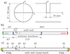Figure 2 (a) Front and side views of the orifice obstructing the upper half of the cross section, (b) full CFD domain and (c) CA domain with indicated sensor positions K1–K6.

The validation experiments were conducted on a small-scale aeroacoustic wind tunnel described in [53]. The setup consists of a long inflow section to ensure fully developed turbulent flow entering the test section, where the orifice is inserted [53]. Anechoic terminations avoid reflections of the acoustic waves, and mufflers reduce the noise of the high-pressure blower, which provides the driving pressure difference. The transient wall pressure is measured by pressure transducers (Kulite XCS-093) for C3. For low flow velocities (C1 and C2), 1/4″ pressure-field microphones (Bruel & Kjaer 4187) are used to capture the wall pressure fluctuations, which the Kulite sensors cannot resolve due to self-noise. More information about the test rig can be found in [53]. The pressure sensors were flush-mounted at the upper side of the pipe (x = 0, y = 25 mm as sketched in Fig. 2c) at the axial positions z stated in Table 2. The sampling rate was 100 kHz corresponding to the CA simulations. The measurement time was t_Exp = 5 s, resulting in N_Exp = 500k samples.

3.3 Flow simulation

3.3.1 Numerical setup

The applied CFD solver uses a second-order accurate Finite Volume discretization in space and a first order implicit scheme in time. The same computational mesh with a total number of 10.5 million elements was used for all cases. The topology of the mesh is presented in Figure 3. The mesh was radially refined towards the wall to reach a high near-wall resolution measured in non-dimensional radial wall distance $\Delta r v_{\tau }/\nu =\Delta r^{+}<1$, referring to the inflow conditions upstream the orifice, as listed in Table 1, where $v_{\tau }=\sqrt{{\tau }_{\mathrm{W}}/\rho }$ is the velocity scale based on the wall shear stress τ_W. The region around the sharp orifice was additionally refined to provide the high spatial resolution required in this region. This highly resolved region is connected with the coarser grids up- and downstream using arbitrary interfaces (see Fig. 2b). Arbitrary interfaces allow for a fully conservative matching of two adjacent non-conforming mesh topologies. At the inlet boundary, an instantaneous velocity profile was imposed, which was generated in a separate precursor LES of fully developed incompressible turbulent pipe flow, at the wall friction based Reynolds number Re_τ = v_τ D/ν as listed in Table 1. At the outlet, an averaged constant pressure was prescribed. No-slip conditions v^ic = 0 were applied at solid walls. A constant time step Δt_CFD was used, and each case was simulated for six flow-through times (t_FT in Tab. 1), with t_FT = L/U representing the time required by a virtual particle to pass the full flow domain of length L at constant bulk velocity U. After convergence was reached, the source terms for the CA simulation time t_CA (see Tab. 1) were exported.

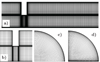Figure 3 CFD mesh: (a) longitudinal view, (b) detail near the orifice, (c) cross-sectional view of the in- and outflow section and (d) cross-sectional view of the refined mesh near the orifice.

3.3.2 Flow simulation results and comparison against measurements

The structure of the flow field is qualitatively shown in Figure 4, displaying contours of the instantaneous and averaged axial velocity ${\tilde{v}}_z^{\mathrm{ic}}$, turbulent kinetic energy ${\tilde{k}}^{\mathrm{ic}}=\frac{1}{2}({\tilde{\mathit{v}}}^{\mathrm{ic}\mathrm{\prime }}\cdot {\tilde{\mathit{v}}}^{\mathrm{ic}\mathrm{\prime }})$, and the incompressible pressure $\tilde{\pi }$ for case C1. The velocity field is strongly accelerated in the lower halfpipe. It detaches at the upstream edge of the orifice, where vortical structures emerge, floating further downstream in a highly turbulent shear layer, as indicated by the instantaneous pressure fluctuations and high turbulent kinetic energy in this region. This shear layer, which represents a region with very intense production of turbulent kinetic energy, separates the high-velocity region at the bottom from the recirculation zone in the wake of the orifice. The separated flow reattaches at the upper wall roughly at z = 3.7D = L_RP downstream of the orifice, indicated by the black vertical line in Figure 4. The reattachment length was determined by the zero of the average axial component of the wall shear stress $\overline{{\tau }_{\mathrm{W},\mathrm{z}}}=0$ along the top wall (x = 0 and y = D/2). The small recirculation zone, which emerges directly from the forward-facing edge of the orifice, effectively further contracts the flow. Downstream of the reattachment, the velocity field recovers towards uniformity again so that the level of turbulence kinetic energy slowly decreases.

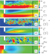Figure 4 Contours of the (a) instantaneous axial velocity ${\tilde{v}}_z^{\mathrm{ic}}$ and its mean value (b) ${\overline{\stackrel{̃}{v}}}_z^{\mathrm{ic}}$, the (c) instantaneous turbulent kinetic energy $\tilde{k}=\frac{1}{2}({\tilde{\mathit{v}}}^{\mathrm{ic\text{'}}}\cdot {\tilde{\mathit{v}}}^{\mathrm{ic\text{'}}})$, and its mean value (d) ${\overline{\stackrel{̃}{k}}}^{\mathrm{ic}}$, (e) the instantaneous pressure fluctuations ${\tilde{\pi }}^{\mathrm{ic\text{'}}}$ and its mean value and (f) ${\overline{\stackrel{̃}{\pi }}}^{\mathrm{ic}}$ for case C1.

For a global validation of the flow simulations, the pressure drop, predicted from LES, is compared against dedicated measurements, as described in Section 3.2. Figure 5 shows the pressure loss coefficients between the positions K1, K2, and K3 defined as $c_{p23}=({\bar{p}}_{K2}-{\bar{p}}_{K3})/\left(\frac{1}{2}\rho U^2\right)$ and $c_{p34}=({\bar{p}}_{K3}-{\bar{p}}_{K4})/\left(\frac{1}{2}\rho U^2\right)$, including the loss coefficient representative for the full domain $c_{p16}=({\bar{p}}_{K1}-{\bar{p}}_{K6})/\left(\frac{1}{2}\rho U^2\right)$ as well. The full loss coefficients and the relative error of the LES predictions to the measurements are listed in Table 3. The predicted pressure loss coefficient over the entire domain shows good agreement for C1 associated with the lowest Reynolds number. With increasing Reynolds number, the predictions increasingly deviate from the measurement. As indicated by the comparison of the coefficient $c_{p23}$, this discrepancy can be largely attributed to an overpredicted pressure drop between the positions immediately upstream and downstream of the orifice, K2 and K3, respectively. As follows from a global momentum balance over the whole domain, this pressure difference ${\bar{p}}_{K2}-{\bar{p}}_{K3}$ mainly determines the total pressure loss over the full domain length $\Delta p_L$. Inside the recirculation zone, the agreement with the measurements is better, as seen from the predicted pressure differences between K3 and K4 represented by $c_{p34}$.

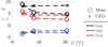Figure 5 Pressure loss coefficients $c_{\mathrm{pL}}=\Delta p_L/\left(\frac{1}{2}\rho U^2\right)$ over the entire domain and between individual axial positions K2, K3, and K4.

Figure 6 presents the Rms of the near-wall pressure fluctuations from LES plotted over the axial coordinate normalized by the reattachment length $L_{\mathrm{RP}}$, including the values measured at the individual measurement positions. For all Reynolds numbers, the Rms values become highest closely upstream of the reattachment point associated with z/L_RP = 0.5 ÷ 1. As can be seen from Figure 4e, this local maximum is evidently generated by the patchy structures of the instantaneous pressure hitting the upper wall. The maximum reached Rms level strongly increases with increasing Reynolds number by orders of magnitude. The measurements, which inherently include the acoustic fluctuations not covered by the incompressible LES, consistently show similar trends with the peak near z/L_RP = 1. The presently observed variation of the pressure fluctuations was typically also observed in experiments on flows over backward-facing step [54]. For step height based Reynolds numbers Re_H = UH/ν > 10⁴, this generic separated flow configuration further showed an invariant reattachment length independent of Re_H, similar to the present configuration, where L_RP was predicted roughly the same for all cases C1, C2 and C3. As indicated by the instantaneous contours in Figure 4e, the pressure fluctuations are predicted much stronger in the highly sheared central layer downstream of the orifice as compared to those near the wall. The pressure fluctuations in the vicinity of the reattachment point are therefore of only minor acoustic relevance, as they effectively generate comparitively weak acoustic source terms. This aspect will also be clearly seen in the source term analysis below.

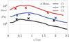Figure 6 Rms of the near-wall pressure ${\tilde{p}}^{\mathrm{ic}}$ over z/LRP from LES and from measurements at positions K3, K4 and K5.

3.3.3 Source term analysis

In the case of incompressible LES, the Lighthill source term defined by (7) is provided only in terms of the resolved, i.e. filtered, velocity field. Decomposing the incompressible velocity into a resolved (${\tilde{\mathit{v}}}^{\mathrm{ic}}$) and an unresolved part (${\mathit{v}}^{\mathrm{ic}\mathrm{\text{'}\text{'}}}$) as

$${\mathit{v}}^{\mathrm{ic}}={\tilde{\mathit{v}}}^{\mathrm{ic}}+{\mathit{v}}^{{\mathrm{ic}}^{\mathrm{\text{'}\text{'}}}}$$(19)

accordingly gives

$$Q_{\mathrm{LH}}^{\mathrm{ic}}=\underset{Q_{\mathrm{LH},\mathrm{RES}}^{\mathrm{ic}}}{\underbrace{{\rho }_0\nabla \cdot \nabla \cdot ({\tilde{\mathit{v}}}^{\mathrm{ic}}\otimes {\tilde{\mathit{v}}}^{\mathrm{ic}})}}+{\rho }_0\nabla \cdot \nabla \cdot ({\mathit{v}}^{\mathrm{ic}\mathrm{\text{'}\text{'}}}\otimes {\tilde{\mathit{v}}}^{\mathrm{ic}}+{\tilde{\mathit{v}}}^{\mathrm{ic}}\otimes {\mathit{v}}^{\mathrm{ic}\mathrm{\text{'}\text{'}}}+{\mathit{v}}^{\mathrm{ic}\mathrm{\text{'}\text{'}}}\otimes {\mathit{v}}^{\mathrm{ic}\mathrm{\text{'}\text{'}}}),$$(20)

where the unresolved contribution is accounted for by the subgrid-scale model for the SGS-stresses defined in (3). Invoking the continuity constraint for incompressible flow, $\nabla \cdot {\tilde{\mathit{v}}}^{\mathrm{ic}}=0$, the source term is finally obtained in the LES as

$$Q_{\mathrm{LH}}^{\mathrm{ic}}\approx {\tilde{Q}}_{\mathrm{LH}}^{\mathrm{ic}}=\underset{{\tilde{Q}}_{\mathrm{LH},\mathrm{RES}}^{\mathrm{ic}}}{\underbrace{{\rho }_0\nabla {\tilde{\mathit{v}}}^{\mathrm{ic}}:(\nabla {\tilde{\mathit{v}}}^{\mathrm{ic}}{)}^{\mathrm{T}}}}+\underset{{\tilde{Q}}_{\mathrm{LH},\mathrm{SGS}}^{\mathrm{ic}}}{\underbrace{\nabla \cdot \left(\nabla \cdot \left(-2{\rho }_0{\nu }_{\mathrm{SGS}}[\tilde{\mathit{S}}{]}^{\mathrm{ic}}\right)\right)}}$$(21)

involving a directly resolved component and a contribution from the SGS model. In the presently applied FV-approach with a collocated grid, the velocity vector v is defined at the centroid of the finite volumes. The velocity gradients needed in (21) were approximated at these points using a second-order Least Square method. In this context, it has to be noted, that in the following source term analysis, the scalar source term $Q_{\mathrm{LH}}^{\mathrm{ic}}$ and its contributions (21) are investigated. For the CA propagation simulation (see Sect. 3.4), the source term vector ${\mathit{q}}_{\mathrm{LH}}^{\mathrm{ic}}$ according to (10) was used instead. The source term vector was obtained from the CFD simulation as

$${\mathit{q}}_{\mathrm{LH}}^{\mathrm{ic}}\approx {\tilde{\mathit{q}}}_{\mathrm{LH}}^{\mathrm{ic}}=\underset{{\tilde{\mathit{q}}}_{\mathrm{LH},\mathrm{RES}}^{\mathrm{ic}}}{\underbrace{{\rho }_0\left(\nabla {\tilde{\mathit{v}}}^{\mathrm{ic}}\right){\tilde{\mathit{v}}}^{\mathrm{ic}}}}+\underset{{\tilde{\mathit{q}}}_{\mathrm{LH},\mathrm{SGS}}^{\mathrm{ic}}}{\underbrace{\nabla \cdot \left(-2{\rho }_0{\nu }_{\mathrm{SGS}}[\tilde{\mathit{S}}{]}^{\mathrm{ic}}\right)}},$$(22)

where the SGS contribution ${\tilde{\mathit{q}}}_{\mathrm{LH},\mathrm{SGS}}^{\mathrm{ic}}$ was neglected in the export.

Figure 7 presents contour plots of the resolved Lighthill source term and the contribution from the SGS model. Both components are especially strong in the highly turbulent shear layer emerging from the detachment on the upstream edge of the orifice. The SGS contribution is always significantly smaller than the resolved component.

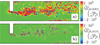Figure 7 Contours of the (a) resolved Lighthill source term ${\tilde{Q}}_{\mathrm{LH},\mathrm{RES}}^{\mathrm{ic}}$ and (b) the SGS contribution ${\tilde{Q}}_{\mathrm{LH},\mathrm{SGS}}^{\mathrm{ic}}$ for case C1. Different ranges are used for the color bars for better visualization.

Figure 8 presents spectra of the full Lighthill source term together with the resolved and the SGS contribution at an arbitrarily chosen position (y = −0.15D, z = −0.73D) inside the highly turbulent region downstream of the orifice, indicated by the cross in Figure 8d. The amplitudes of the SGS contribution to the Lighthill source term are consistently one order of magnitude smaller than the resolved contribution up to frequencies of f ≈ 10 kHz, which demonstrates their quantitative irrelevance in the full Lighthill source term, as also shown in [55]. This is also true for the case C3 with the highest Reynolds number, where the modelled unresolved part of the turbulent kinetic energy is largest. The relative contribution to the source term is also insignificant in this case. Therefore, the SGS contribution is not included in the exported source terms for the CA simulation.

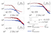Figure 8 Spectra of the resolved, SGS contribution and full Lighthill source term for (a) C1, (b) C2 and (c) C3, inside the high turbulent region marked in (d).

The PCWE source term is computed from the resolved instantaneous incompressible pressure ${\tilde{\pi }}^{\mathrm{ic}\mathrm{\prime }}$ as

$${\tilde{Q}}_{\mathrm{PCWE}}^{\mathrm{ic}}=-\underset{{\tilde{Q}}_{\mathrm{PCWE},\mathrm{t}}^{\mathrm{ic}}}{\underbrace{\frac{1}{\rho c^2}\left(\frac{\mathrm{\partial }{\tilde{\pi }}^{{\mathrm{ic}}^{\mathrm{\prime }}}}{\mathrm{\partial }t}\right)}}-\underset{{\tilde{Q}}_{\mathrm{PCWE},\mathrm{c}}^{\mathrm{ic}}}{\underbrace{\frac{1}{\rho c^2}\left({\overline{\stackrel{̃}{\mathit{v}}}}^{\mathrm{ic}}\cdot \nabla {\tilde{\pi }}^{{\mathrm{ic}}^{\mathrm{\prime }}}\right)}},$$(23)

where ${\overline{\stackrel{̃}{\mathit{v}}}}^{\mathrm{ic}}$ represents the time averaged resolved incompressible velocity from LES. Figure 9 presents contours of the PCWE source term and its components for case C1. Similar to the structures of the underlying instantaneous incompressible pressure field, which are emerging from the upstream edge of the orifice as observed in Fig. 4, alternating patch-like structures appear in the highly turbulent shear layer confining the separated flow region. Both the component ${\tilde{Q}}_{\mathrm{PCWE},\mathrm{t}}^{\mathrm{ic}}$ and component ${\tilde{Q}}_{\mathrm{PCWE},\mathrm{c}}^{\mathrm{ic}}$ significantly contribute in this layer, however mostly opposite in sign, which effectively produces more fine-grained structures in the resulting total PCWE source term ${\tilde{Q}}_{\mathrm{PCWE}}^{\mathrm{ic}}$ [47].

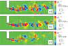Figure 9 Contours of the PCWE source term and its components for case C1.

Figure 10 shows spectra of the PCWE source term and its components at two arbitrarily selected positions (P1 and P2 at y_P1 = 0.045D, y_P2 = −0.36D and z_P1−2 = 1.27D) downstream of the orifice for all cases. For case C2, two additional points (P3 and P4 at y_P3 = 0.36D, z_P3 = 1.27D and y_P4 = 0.045D, z_P4 = 3.27D) were considered to analyze also the conditions inside the separated flow region and in the central core region further downstream. At position P1, directly inside the highly turbulent shear layer downstream of the orifice, the convective component ${\tilde{Q}}_{\mathrm{PCWE},\mathrm{c}}^{\mathrm{ic}}$ is significantly weaker than the time derivative component ${\tilde{Q}}_{\mathrm{PCWE},\mathrm{t}}^{\mathrm{ic}}$, so that the resulting full source term ${\tilde{Q}}_{\mathrm{PCWE}}^{\mathrm{ic}}$ is dominated by the latter. This can be explained by the low mean velocity in this region (see Fig. 4). In the high-velocity region at P2, rather the convective contribution is dominating up to high frequencies of f < 5000 Hz, where the time derivative term gains dominance according to the dimensional analysis (16). Moreover, beyond f = 200, 300 and 600 Hz, for case C1, C2 and C3 respectively, the amplitudes of the total source term are always significantly smaller than the amplitudes of its constitutive components, indicating that these contributions are negatively correlated in this region and thus tend to cancel each other. At P3, inside the recirculation zone, and further downstream at P4, the components have similar amplitudes up to f = 2000 Hz and the total source term is smaller than its components. For the high frequencies above f = 3000 Hz, the time derivative term becomes dominant again, as expected from (16). The observed mutual cancelling of the two constituent components of the PCWE source term is further analyzed in Figure 11, presenting cross-correlation profiles of the total PCWE source term and its components as a function of the normalized y coordinate at selected positions z. The correlation coefficients are obtained from the local temporal signals as

$$X\left\{\mathrm{\Phi },\mathrm{\Psi }\right\}=\frac{\overline{{\mathrm{\Phi }}^{\mathrm{\prime }}{\mathrm{\Psi }}^{\mathrm{\prime }}}}{\sqrt{\overline{{\mathrm{\Phi }}^{\mathrm{\prime }2}}}\sqrt{\overline{{\mathrm{\Psi }}^{\mathrm{\prime }2}}}}.$$(24)

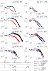Figure 10 Spectra of the PCWE source term and its components within the high turbulent region (P1) and the high-velocity region (P1) marked in the bottom subfigure, for (a) and (b) C1, (c) and (d) C2, (e) and (f) C3, respectively. Additional spectra for C2 inside the (g) recirculation zone and (h) further downstream of the high turbulent region (P4).

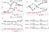Figure 11 Cross-correlation profiles of the PCWE source terms and its components along the y-axis for case C1 at positions (a) z = 1.27D, (b) 3.27D and (c) 6.27D.

The variation at z = 1.27D, which also carries the points P1–3 analyzed above, indicates effectively uncorrelated time derivative and convective components in the shear layer near y/R=0.3. In the high-velocity region towards the lower wall, the time derivative and convective components become strongly negatively correlated, as $X\{{\tilde{Q}}_{\mathrm{PCWE},\mathrm{t}}^{\mathrm{ic}},{\tilde{Q}}_{\mathrm{PCWE},\mathrm{c}}^{\mathrm{ic}}\}\sim -1$. The total source terms is essentially dominated here by the convective contribution, as indicated by the almost unity value of $X\{{\tilde{Q}}_{\mathrm{PCWE}}^{\mathrm{ic}},{\tilde{Q}}_{\mathrm{PCWE},\mathrm{c}}^{\mathrm{ic}}\}$. The observed trends of $X\{{\tilde{Q}}_{\mathrm{PCWE},\mathrm{t}}^{\mathrm{ic}},{\tilde{Q}}_{\mathrm{PCWE},\mathrm{c}}^{\mathrm{ic}}\}$ towards $-1$, when approaching the lower and upper walls, clearly reflects the mutual cancelling of the time derivative and convective components seen in the spectra at the points P2 and P3 in Figure 10. Further downstream at z = 3.27D, the location of highly uncorrelated convective and time derivative components is moved towards the upper wall following essentially the position of the shear layer, which confines the separated flow region. Towards the lower wall, this correlation drops again to −1. Accordingly, a strong mutual cancelling of ${\tilde{Q}}_{\mathrm{PCWE},\mathrm{t}}^{\mathrm{ic}}$ and ${\tilde{Q}}_{\mathrm{PCWE},\mathrm{c}}^{\mathrm{ic}}$ was observed in the spectra of point P4 in Figure 10. Further downstream of the reattachment at z = 6.27D the cross-correlation coefficients finally remains always very close to −1. The mutual cancelling of the time derivative and convective component in P2–4 suggests that Taylor’s hypothesis of “frozen turbulence”, which basically requires ${\tilde{v}}_z^{\mathrm{ic}\mathrm{\prime }}\ll {\overline{\stackrel{̃}{v}}}_z^{\mathrm{ic}}$ (see Fig. 4) [56, 57], is largely applicable also in the present complex separated flow. The impact of this cancellation, which has also been reported for mixing layer sound generation in [58], on the resulting acoustic field of the present configuration will be illustrated in the analysis below.

3.4 Acoustic simulation

3.4.1 Numerical setup

The computational grid for the CA simulation displayed in Figure 12 covers the fluid domain, which includes the CFD domain containing the source terms and the adjacent PML regions, which absorb outgoing acoustic waves without reflections. The structured hexahedral mesh consists of a total of approximately 133k linear elements, where 131k belong to the fluid region and 1k to each of the two adjacent PML regions. The cell size is approximately 2.8 mm, discretizing the acoustic wavelength λ_min = c₀/f_max by 15 finite elements, where f_max = 8 kHz is the upper frequency limit for the evaluation of the spectral CA results.

Figure 12 CA mesh with consisting of a fluid region (grey) and adjacent PML regions (yellow).

For the temporal discretization, the Newmark method implemented in openCFS and a time step size of Δt_CA = 10 μs simulation were chosen. The temporal blending function

$$b\left(t\right)=(\begin{array}{ll}{\sin }^2\left(\frac{\frac{\pi }{2}}{80\Delta t}t\right)& \mathrm{for} t\le 80\Delta t\\ 1& \mathrm{else}\end{array},$$(25)

depending on the simulation time t was defined to smoothly activate the acoustic sources during the first 80 time steps to avoid impulsive excitation [13]. The CA simulation time for the cases C1 and C2 was t_CA = 0.2 s, and for C3 t_CA = 0.1 s (see Tab. 1) resulting in N_CA = 20k and N_CA = 10k time steps, respectively.

3.4.2 Propagation simulation results and comparison against measurements

The pressure fluctuations are investigated in the frequency domain computing the Power Spectral Density (PSD) based on Welch’s method [59], where a Hamming window is applied to each segment of length N_W = 3000 with an overlap of 50%. For an adequate comparison, the same procedure was applied to 50%-overlapping segments of the measurement data with the same length as the CA simulation t_CA. The therefrom obtained set of PSDs $P_{\mathrm{P}\mathrm{SD},i}^{\mathrm{m}\mathrm{eas}}\left(f\right)$, as well as their mean ${\bar{P}}_{\mathrm{P}\mathrm{SD}}^{\mathrm{m}\mathrm{eas}}\left(f\right)$, are used for the validation of the simulations, where a frequency range of f_min = 100 kHz ≤ f ≤ f_max = 8 kHz is considered. Figure 13 displays the CA simulation results of the three cases at the position K2 upstream of the orifice and K4 downstream of the orifice. Therein, the spectra of the segments of the measurement $P_{\mathrm{PSD},i}^{\mathrm{meas}}\left(f\right)$ are displayed in grey and their mean ${\bar{P}}_{\mathrm{PSD}}^{\mathrm{meas}}\left(f\right)$ in black. Since the pressure transducers measure the total pressure fluctuation, the time signal of the incompressible pressure from the flow simulation is added to the acoustic pressure obtained from the CA simulation according to (13) for PCWE and RIB before determining the PSD of the simulation $P_{\mathrm{PSD}}^{\mathrm{sim}}\left(f\right)$. The natural frequencies f_mn of the acoustic higher-order modes are indicated in the spectra, which can be derived analytically for an infinitely long circular pipe with uniform mean flow [60]. The index m denotes the circumferential order, and n the radial order of the mode. The excitation of these acoustic modes can be clearly seen within the spectra, especially in the upstream position, where less turbulent pressure fluctuation is superimposed.

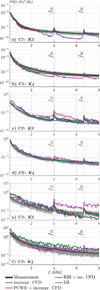Figure 13 PSDs of the wall pressures of C1, C2, and C3 at positions upstream (K2) and downstream (K4) of the orifice.

In Figure 14, the real part of the Fourier transform of the acoustic field obtained by the PCWE for C1 at position K2 is visualized for f₁₀ and f₂₀, which clearly exhibit the expected mode shapes of first and second circumferential order. The pressure sensor at K4 is located directly in the source region downstream of the orifice. The enhanced turbulent motion in this region increases the noise within the spectra, especially in the higher frequency range, and thus, makes the peaks of the acoustic higher order modes less pronounced. The spectra are generally predicted appropriately by the LES, apart from the acoustic peaks, which are not captured due to the incompressible flow assumption. When adding the acoustic pressure predicted by RIB and PCWE to the incompressible pressure of the LES according to (13), the resulting spectra match the measurements well. Furthermore, the matching spectra of RIB and PCWE indicate that convective effects can be neglected for the considered flow rates. This can be explained by the low Mach number of the considered cases (see Tab. 2), which scales the convective term according to (16). The CA simulation of LH solving for the total pressure fluctuations p$\mathrm{\prime }$ inherently includes the incompressible pressure fluctuations, added with the contribution of the acoustic wave propagation arising from compressibility. The spectra partly deviate from the measurements in the higher frequency range. This is thought to be caused by the non-conservative least-squares approach used for computation of the spatial derivatives of the LH source term, as described in [14]. The instantaneous pressure fields depicted in Figure 15 show that the incompressible pressure fluctuations, which are the dominating part, are reproduced well by LH. The acoustic pressure fluctuations added in the LH simulation occurring in the higher frequency range are not visible because they are several orders of magnitude lower. In contrast, the resulting pressure fields of RIB and PCWE depicted in Figure 16 clearly exhibit a purely wave-like, acoustic behavior, as expected. Figure 17 shows the contributions of the PCWE to the PSD of the total pressure (PCWE full + incompr. CFD) from the case C2 at two sensor positions downstream of the orifice. For better visibility, only the average PSD of the measurement is plotted. The resulting spectra of the CA simulation with only the time derivative source term ${\tilde{Q}}_{\mathrm{PCWE},\mathrm{t}}^{\mathrm{ic}}$ match the simulation with the total source term ${\tilde{Q}}_{\mathrm{PCWE}}^{\mathrm{ic}}$, revealing that the impact of the convective source term ${\tilde{Q}}_{\mathrm{PCWE},\mathrm{c}}^{\mathrm{ic}}$ is negligible. This indicates that the source term part, being canceled out due to the negative correlation of the source term components ${\tilde{Q}}_{\mathrm{PCWE},\mathrm{t}}^{\mathrm{ic}}$ and ${\tilde{Q}}_{\mathrm{PCWE},\mathrm{c}}^{\mathrm{ic}}$, does not significantly contribute to sound generation. The incompressible component dominates the total pressure fluctuations at position K4. At K6 (17D downstream of the orifice) these incompressible pressure fluctuations are decayed, and the spectrum is governed by the acoustic part, which is well resolved by the PCWE.

Figure 14 Real part of the Fourier transform of the acoustic pressure obtained by the PCWE for C1 at f10 = 4044.7 Hz (left) and f20 = 6709.6 Hz (right).

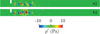Figure 15 Instantaneous field of pressure fluctuation of C1 of (a) the propagation simulation and of (b) the incompressible CFD simulation at t = 0.03 s.

Figure 16 Instantaneous field of the acoustic pressure of C1 obtained by (a) the PCWE-based propagation simulation and (b) by the RIB-based propagation simulation at t = 0.03 s.

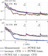Figure 17 PSDs of the wall pressures for case C2 at positions K4 and K6 downstream of the orifice.

To quantify the accuracy of the simulation results, a logarithmic error

$$E_{\log }^{\mathrm{sim}}=\frac{1}{f_{\max }-f_{\min }}\underset{f_{\min }}{\overset{f_{\max }}{\int }}\mathrm{}\frac{d_{\log }\left(f\right)}{{\sigma }_{\log }^{\mathrm{meas}}\left(f\right)} \mathrm{d}f$$(26)

is introduced, where the logarithmic deviation

$$d_{\log }\left(f\right)=\left|\log \left({\bar{P}}_{\mathrm{PSD}}^{\mathrm{meas}}\left(f\right)\right)-\log \left(P_{\mathrm{PSD}}^{\mathrm{sim}}\left(f\right)\right)\right|.$$(27)

is related to the logarithmic standard deviation ${\sigma }_{\log }^{\mathrm{meas}}(\log \left(P_{\mathrm{PSD},i}^{\mathrm{meas}}\left(f\right)\right)$ of the set of PSDs $P_{\mathrm{PSD},i}^{\mathrm{meas}}$. Table 4 shows that except for LH in case C1, the accuracy of the incompressible CFD simulation is enhanced when applying the hybrid approach since the error is reduced. PCWE and RIB achieved similar results with a smaller error than LH. For PCWE and RIB, the spectra are predicted more accurately for the smaller flow rates, which is in line with the predicted pressure drop (Tab. 3). This confirms the expectation that an accurate CFD simulation is crucial for the hybrid approach, since it is the basis for the computation of the acoustic sources. Additionally, the flow-induced sound is specified in Table 4 in terms of the Sound Pressure Level (SPL) computed as

$$L_{p^{\mathrm{a}}}=20 \log \frac{p_{\mathrm{Rms}}^{\mathrm{a}}}{p_{\mathrm{ref}}^{\mathrm{a}}},$$(28)

to quantify the flow-induced sound depending on the flow speed. The reference pressure $p_{\mathrm{ref}}^{\mathrm{a}}=20 \mathrm{\mu }\mathrm{s}$ and the Rms of the acoustic pressure signals $p_{\mathrm{Rms}}^{\mathrm{a}}=\mathrm{Rms}\left(p^{\mathrm{a}}\right)$ predicted by PCWE and RIB were used for evaluation. The results show that already a substantial SPL of about 80 dB is produced by the relatively small flow velocity of C1 $\left(U=3.87 \frac{\mathrm{m}}{\mathrm{s}}\right)$ going up to approximately 120 dB of C3 $\left(U=20.79 \frac{\mathrm{m}}{\mathrm{s}}\right)$. Furthermore, the comparison of the SPLs of the specific cases emphasizes the equivalence of PCWE and RIB in the present application.

4 Practical aspects

As for the practical application of the hybrid approach, one major challenge is the efficient coupling of the CFD simulation with the CA simulation, especially if different simulation tools are used. The amount of acoustic source data to be generated, stored, and transferred from the instantaneous spatially highly resolved CFD solution to the CA solver should be kept lowest. In the present setting, the source terms were conservatively mapped from the fine CFD to the coarse CA mesh before the export, thus reducing the amount of transferred data significantly. More precisely, the data set of a scalar quantity of a single timestep (TS) was reduced from 91 MB (CFD grid) to 1 MB (CA grid). Additionally, the sources were exported in time increments determined by the CA time step, so that for the cases C2 and C3, where $\Delta t_{\mathrm{CA}}>\Delta t_{\mathrm{CFD}}$, the instants of time for data export essentially remained the same, always based on Δt_CA, which was not altered for the considered cases. The CFD simulation was performed using 128 CPUs (AMD EPYC 7702) and took approximately $t_{\mathrm{sol}}^{\mathrm{CFD}}=28 \mathrm{s}$ per CFD timestep for solving the flow field using approximately 515 GB of memory. The export of one scalar source term to the CA grid took t_exp = 6 s per CA timestep, where 99.7% of the time is required for data mapping from the fine CFD mesh to the coarse CA mesh, and 0.3% for writing the data to hdf5-files. In comparison, solving one time step in the CA simulation only took $t_{\mathrm{sol}}^{\mathrm{CA}}=0.8 \mathrm{s}$ using 4 CPUs (Intel Xeon G 5218) with an approximate memory usage of 1.5 GB. The computational resources required by the respective steps in the simulation workflow are summarized in Table 5.

5 Conclusions

Three hybrid aeroacoustic formulations were applied to a confined flow through a circular pipe (D = 50 mm) with a half-moon-shaped orifice using the CFD code AVL FIRE™ and the FE solver openCFS. Based on the results of the incompressible flow simulation, an extensive analysis of the source terms and sound generation mechanisms was provided. The LES predicted a highly turbulent shear layer downstream of the orifice, emerging from the detachment at the upstream edge of the orifice. Downstream of the orifice, the shear layer separates the high-velocity region caused by the flow contraction from the recirculation zone in the wake of the half-moon-shaped obstacle. Vortical structures emerging from the detachment appear within this sheared region causing high pressure and velocity fluctuations. This leads to the strongest source terms in this region. The SGS contribution to the Lighthill source terms is insignificantly small at lower frequencies. It was shown that convective effects can be neglected in the acoustic propagation simulation, although the convective PCWE source term significantly reduces the total source term due to negative correlation with the time derivative term especially in the high-velocity region below the separating shear layer.

The study revealed that the PCWE and RIB are best suited for the present task, having a small deviation of 2.26 and 2.13, respectively, with respect to the standard deviation of the measurement, compared to LH with 3.55. Besides reliably predicting the flow-induced sound, the source term computation is straightforward and can easily be implemented in commercial solvers. Despite the slightly better accuracy, the PCWE is preferred over RIB, especially for higher flow velocities. It is thought to predict more accurate results because of considering the convection of acoustic waves, and thus being applicable more generally. Furthermore, the source term of Ribner’s Dilatation equation contains the second time derivative of the incompressible pressure and therefore, is more sensitive to small-scale temporal variations in the transient incompressible pressure signals used as input. Since the convective source term was shown to be negligible for the considered flow rates, the PCWE source term is simply made up by the first time derivative of the incompressible pressure, and no filtering is required. In contrast, the LH source term involves spatial derivatives and, thus, is strongly dependent on the spatial resolution. Furthermore, the temporal mean value must be removed in a filtering process. On the other hand, LH directly yields the total pressure fluctuations, which are, for example, required when mechanical coupling to the flow guiding structure is considered. Therefore, the computation of the spatial derivatives using conservative schemes will be investigated in the future. Analysis of the computational times showed that the export of source term data on the CA grid drastically reduces the computational effort.

Conflict of interest

The authors declare no conflict of interest.

Acknowledgments

The support from the Austrian Research Promotion Agency (FFG) under no. 874784 and from AVL List GmbH Graz are gratefully acknowledged. Supported by TU Graz Open Access Publishing Fund.

References

All Tables

All Figures

	Figure 1 CAA simulation workflow applied in the hybrid approach.
In the text

	Figure 2 (a) Front and side views of the orifice obstructing the upper half of the cross section, (b) full CFD domain and (c) CA domain with indicated sensor positions K1–K6.
In the text

	Figure 3 CFD mesh: (a) longitudinal view, (b) detail near the orifice, (c) cross-sectional view of the in- and outflow section and (d) cross-sectional view of the refined mesh near the orifice.
In the text

Figure 4 Contours of the (a) instantaneous axial velocity ${\tilde{v}}_z^{\mathrm{ic}}$ and its mean value (b) ${\overline{\stackrel{̃}{v}}}_z^{\mathrm{ic}}$, the (c) instantaneous turbulent kinetic energy $\tilde{k}=\frac{1}{2}({\tilde{\mathit{v}}}^{\mathrm{ic\text{'}}}\cdot {\tilde{\mathit{v}}}^{\mathrm{ic\text{'}}})$, and its mean value (d) ${\overline{\stackrel{̃}{k}}}^{\mathrm{ic}}$, (e) the instantaneous pressure fluctuations ${\tilde{\pi }}^{\mathrm{ic\text{'}}}$ and its mean value and (f) ${\overline{\stackrel{̃}{\pi }}}^{\mathrm{ic}}$ for case C1.

In the text

	Figure 5 Pressure loss coefficients $c_{\mathrm{pL}}=\Delta p_L/\left(\frac{1}{2}\rho U^2\right)$ over the entire domain and between individual axial positions K2, K3, and K4.
In the text

	Figure 6 Rms of the near-wall pressure ${\tilde{p}}^{\mathrm{ic}}$ over z/LRP from LES and from measurements at positions K3, K4 and K5.
In the text

	Figure 7 Contours of the (a) resolved Lighthill source term ${\tilde{Q}}_{\mathrm{LH},\mathrm{RES}}^{\mathrm{ic}}$ and (b) the SGS contribution ${\tilde{Q}}_{\mathrm{LH},\mathrm{SGS}}^{\mathrm{ic}}$ for case C1. Different ranges are used for the color bars for better visualization.
In the text

	Figure 8 Spectra of the resolved, SGS contribution and full Lighthill source term for (a) C1, (b) C2 and (c) C3, inside the high turbulent region marked in (d).
In the text

	Figure 9 Contours of the PCWE source term and its components for case C1.
In the text

	Figure 10 Spectra of the PCWE source term and its components within the high turbulent region (P1) and the high-velocity region (P1) marked in the bottom subfigure, for (a) and (b) C1, (c) and (d) C2, (e) and (f) C3, respectively. Additional spectra for C2 inside the (g) recirculation zone and (h) further downstream of the high turbulent region (P4).
In the text

	Figure 11 Cross-correlation profiles of the PCWE source terms and its components along the y-axis for case C1 at positions (a) z = 1.27D, (b) 3.27D and (c) 6.27D.
In the text

	Figure 12 CA mesh with consisting of a fluid region (grey) and adjacent PML regions (yellow).
In the text

	Figure 13 PSDs of the wall pressures of C1, C2, and C3 at positions upstream (K2) and downstream (K4) of the orifice.
In the text

	Figure 14 Real part of the Fourier transform of the acoustic pressure obtained by the PCWE for C1 at f10 = 4044.7 Hz (left) and f20 = 6709.6 Hz (right).
In the text

	Figure 15 Instantaneous field of pressure fluctuation of C1 of (a) the propagation simulation and of (b) the incompressible CFD simulation at t = 0.03 s.
In the text

	Figure 16 Instantaneous field of the acoustic pressure of C1 obtained by (a) the PCWE-based propagation simulation and (b) by the RIB-based propagation simulation at t = 0.03 s.
In the text

	Figure 17 PSDs of the wall pressures for case C2 at positions K4 and K6 downstream of the orifice.
In the text

References

- D. Siano, M. Prati, M. Costagliola, M. Panza: Evaluation of noise level inside cab of a bi-fuel passenger vehicle. WSEAS Transactions on Applied and Theoretical Mechanics 10 (2015) 220–226. [Google Scholar]
- R. Fan, G. Meng, J. Yang, C. He: Internal noise reduction in railway carriages: A case study in China. Transportation Research Part D: Transport and Environment 13 (2008) 213–220. [CrossRef] [Google Scholar]
- F. Letourneaux, S. Guerrand, F. Poisson: Assessment of the acoustical comfort in high-speed trains at the SNCF: integration of subjective parameters. Journal of Sound and Vibration 231 (2000) 839–846. [CrossRef] [Google Scholar]
- D. Swart, A. Bekker: The relationship between consumer satisfaction and psychoacoustics of electric vehicle signature sound. Applied Acoustics 145 (2019) 167–175. [CrossRef] [Google Scholar]
- D.-U. Yun, S.-K. Lee: Objective evaluation of the knocking sound of a diesel engine considering the temporal and frequency masking effect simultaneously. Journal of Sound and Vibration 397 (2017) 282–297. [CrossRef] [Google Scholar]
- F.G. Praticò, P.G. Briante, G. Speranza: Acoustic impact of electric vehicles, in 2020 IEEE 20th Mediterranean Electrotechnical Conference (MELECON), IEEE, 2020, pp. 7–12. [CrossRef] [Google Scholar]
- D. Siwiak, F. James: Designing interior audio cues for hybrid and electric vehicles, in Audio Engineering Society Conference: 36th International Conference: Automotive Audio, Audio Engineering Society, 2009. [Google Scholar]
- X. Chen, J. Lin, H. Jin, Y. Huang, Z. Liu: The psychoacoustics annoyance research based on EEG rhythms for passengers in high-speed railway. Applied Acoustics 171 (2021) 107575. [CrossRef] [Google Scholar]
- K. Genuit: Particular importance of psychoacoustics for sound design of quiet vehicles, in INTER-NOISE and NOISE-CON Congress and Conference Proceedings, Institute of Noise Control Engineering, vol. 2011, 2011, pp. 2908–2914. [Google Scholar]
- S. Schoder, M. Kaltenbacher: Hybrid aeroacoustic computations: state of art and new achievements. Journal of Theoretical and Computational Acoustics 27 (2019) 1950020. [CrossRef] [Google Scholar]
- T. Colonius: Modeling artificial boundary conditions for compressible flow. Annual Review of Fluid Mechanics 36 (2004) 315–345. [CrossRef] [Google Scholar]
- M. Piellard, B. Coutty: Application of a hybrid computational aeroacoustics method to an automotive blower, in Vehicle Thermal Management Systems Conference and Exhibition (VTMS10), Woodhead Publishing, 2011, pp. 447–455. [CrossRef] [Google Scholar]
- S. Schoder, C. Junger, M. Kaltenbacher: Computational aeroacoustics of the EAA benchmark case of an axial fan: Acta Acustica 4 (2020) 22. [CrossRef] [EDP Sciences] [Google Scholar]
- M. Tautz, K. Besserer, S. Becker, M. Kaltenbacher: Source formulations and boundary treatments for Lighthill’s analogy applied to incompressible flows. AIAA Journal 56 (2018) 2769–2781. [CrossRef] [Google Scholar]
- M. Kaltenbacher, M. Escobar, S. Becker, I. Ali: Numerical simulation of flow-induced noise using LES/SAS and Lighthill’s acoustic analogy. International Journal for Numerical Methods in Fluids 63 (2010) 1103–1122. [Google Scholar]
- A.A. Oberai, F. Roknaldin, T.J. Hughes: Computational procedures for determining structural-acoustic response due to hydrodynamic sources. Computer Methods in Applied Mechanics and Engineering 190 (2000) 345–361. [Google Scholar]
- S. Schoder, M. Weitz, P. Maurerlehner, A. Hauser, S. Falk, S. Kniesburges, M. Döllinger, M. Kaltenbacher: Hybrid aeroacoustic approach for the efficient numerical simulation of human phonation. The Journal of the Acoustical Society of America 147 (2020) 1179–1194. [CrossRef] [PubMed] [Google Scholar]
- S. De Reboul, N. Zerbib, A. Heather: Use openFOAM coupled with finite and boundary element formulations for computational aero-acoustics for ducted obstacles, in INTER-NOISE and NOISE-CON Congress and Conference Proceedings, vol. 259, Institute of Noise Control Engineering, 2019, pp. 4811–4826. [Google Scholar]
- S. De Reboul, E. Perrey-Debain, S. Moreau, N. Zerbib: Hybrid methods for duct aeroacoustics simulations, in Forum Acusticum, Lyon, France, December, 2020, pp. 387–391. [Google Scholar]
- J. Ryu, C. Cheong, S. Kim, S. Lee: Computation of internal aerodynamic noise from a quick-opening throttle valve using frequency-domain acoustic analogy. Applied Acoustics 66 (2005) 1278–1308. [CrossRef] [Google Scholar]
- F. Crouzet, P. Lafon, T. Buchal, D. Laurence: Aerodynamic noise prediction in internal flows using LES and linear Euler equations, in 8th AIAA/CEAS Aeroacoustics Conference & Exhibit, Breckenridge, Colorado, USA, June, 2002, p. 2568. [Google Scholar]
- M. Piellard, C. Bailly: Validation of a hybrid CAA method. Application to the case of a ducted diaphragm at low Mach number, in 14th AIAA/CEAS Aeroacoustics Conference (29th AIAA Aeroacoustics Conference), 2008, p. 2873. [Google Scholar]
- C. Bailly, P. Lafon, S. Candel: Computation of noise generation and propagation for free and confined turbulent flows, in Aeroacoustics Conference, State College, Pennsylvania, USA, May, 1996, p. 1732. [Google Scholar]
- M. Bayati, M. Tadjfar: High Helmholtz sound prediction generated by confined flows and propagation within ducts. International Journal of Acoustics and Vibration 312 (2015) 47. [Google Scholar]
- S. Benhamadouche, M. Arenas, W. Malouf: Wall-resolved large eddy simulation of a flow through a square-edged orifice in a round pipe at Re = 25,000. Nuclear Engineering and Design 312 (2017) 128–136. [CrossRef] [Google Scholar]
- O. Kårekull, G. Efraimsson, M. Åbom: Prediction model of flow duct constriction noise. Applied Acoustics 82 (2014) 45–52. [CrossRef] [Google Scholar]
- E. Longatte, P. Lafon, S. Candel: Computation of noise generation by turbulence in internal flows, in 4th AIAA/CEAS Aeroacoustics Conference, Toulouse, France, June, 1998, p. 2332. [Google Scholar]
- W. Zhao, C. Zhang, S.H. Frankel, L. Mongeau: Computational aeroacoustics of phonation, part I: computational methods and sound generation mechanisms. The Journal of the Acoustical Society of America 112 (2002) 2134–2146. [CrossRef] [PubMed] [Google Scholar]
- M. Bull, N. Agarwal: Characteristics of the flow separation due to an orifice plate in fully-developed turbulent pipe-flow, in Proc. 8th Australasian Fluid Mechanics Conference, University of Newcastle, Australia, 1983. [Google Scholar]
- R. Lacombe, P. Moussou, S. Föller, G. Jasor, W. Polifke, Y. Aurégan: Experimental and numerical investigations on the whistling ability of an orifice in a flow duct, in Exergy, Cairo, Egypt, vol. 2. July, 2010, p. 1. [Google Scholar]
- S. Sack: Experimental and numerical multi-port eduction for duct acoustics. PhD thesis, KTH Royal Institute of Technology, Stockholm, 2017. [Google Scholar]
- P. Testud, Y. Aurégan, P. Moussou, A. Hirschberg: The whistling potentiality of an orifice in a confined flow using an energetic criterion. Journal of Sound and Vibration 325 (2009) 769–780. [CrossRef] [Google Scholar]
- M. Piellard, C. Bailly: Several computational aeroacoustics solutions for the ducted diaphragm at low Mach number, in 16th AIAA/CEAS Aeroacoustics Conference, Stockholm, Sweden, June, 2010, p. 3996. [Google Scholar]
- X. Gloerfelt, P. Lafon: Direct computation of the noise induced by a turbulent flow through a diaphragm in a duct at low Mach number. Computers & Fluids 37 (2008) 388–401. [CrossRef] [Google Scholar]
- R. Fearn, T. Mullin, K. Cliffe: Nonlinear flow phenomena in a symmetric sudden expansion. Journal of Fluid Mechanics 211 (1990) 595–608. [CrossRef] [Google Scholar]
- F. Durst, J. Pereira, C. Tropea: The plane symmetric sudden-expansion flow at low Reynolds numbers. Journal of Fluid Mechanics 248 (1993) 567–581. [CrossRef] [Google Scholar]
- E. Wahba: Iterative solvers and inflow boundary conditions for plane sudden expansion flows. Applied mathematical modelling 31 (2007) 2553–2563. [CrossRef] [Google Scholar]
- C. Bogey, C. Bailly, D. Juvé: Computation of flow noise using source terms in linearized Euler’s equations. AIAA Journal 40 (2002) 235–243. [CrossRef] [Google Scholar]
- M. Kaltenbacher: Numerical simulation of mechatronic sensors and actuators: finite elements for computational multiphysics, vol. 3, Springer, 2015. [Google Scholar]
- H. Kobayashi: The subgrid-scale models based on coherent structures for rotating homogeneous turbulence and turbulent channel flow. Physics of Fluids 17 (2005) 045104. [CrossRef] [Google Scholar]
- H. Kobayashi, F. Ham, X. Wu: Application of a local SGS model based on coherent structures to complex geometries. International Journal of Heat and Fluid Flow 29 (2008) 640–653. [CrossRef] [Google Scholar]
- M.J. Lighthill: On sound generated aerodynamically I. General theory. Proceedings of the Royal Society of London. Series A. Mathematical and Physical Sciences 211 (1952) 564–587. [Google Scholar]
- B. Kaltenbacher, M. Kaltenbacher, I. Sim: A modified and stable version of a perfectly matched layer technique for the 3-d second order wave equation in time domain with an application to aeroacoustics. Journal of Computational Physics 235 (2013) 407–422. [CrossRef] [PubMed] [Google Scholar]
- R. Ewert, W. Schröder: Acoustic perturbation equations based on flow decomposition via source filtering. Journal of Computational Physics 188 (2003) 365–398. [Google Scholar]
- A. Hüppe, J. Grabinger, M. Kaltenbacher, A. Reppenhagen, G. Dutzler, W. Kühnel: A non-conforming finite element method for computational aeroacoustics in rotating systems, in 20th AIAA/CEAS Aeroacoustics Conference, Atlanta, Georgia, USA, June, 2014, pp. 2014–2739. [Google Scholar]
- M. Kaltenbacher, A. Hüppe, A. Reppenhagen, F. Zenger, S. Becker: Computational aeroacoustics for rotating systems with application to an axial fan. AIAA Journal 55 (2017) 3831–3838. [Google Scholar]
- S. Schoder, P. Maurerlehner, A. Wurzinger, A. Hauser, S. Falk, S. Kniesburges, M. Döllinger, M. Kaltenbacher: Aeroacoustic sound source characterization of the human voice production-perturbed convective wave equation. Applied Sciences 11 (2021) 2614. [CrossRef] [Google Scholar]
- H.S. Ribner: Aerodynamic sound from fluid dilatations: A theory of the sound from jets and other flows. UTIA Report, No. 86, 1962. AFOSR TN 3430 [Google Scholar]
- AVL FIRE™: 2022. www.avl.com/fire [Google Scholar]
- S. Schoder, A. Wurzinger, C. Junger, M. Weitz, C. Freidhager, K. Roppert, M. Kaltenbacher: Application limits of conservative source interpolation methods using a low Mach number hybrid aeroacoustic workflow. Journal of Theoretical and Computational Acoustics 29, 01 (2021) 2050032. [CrossRef] [Google Scholar]
- openCFS – finite element multiphysics solver, 2022. www.opencfs.org [Google Scholar]
- W. Sutherland: The viscosity of gases and molecular force. The London, Edinburgh, and Dublin Philosophical Magazine and Journal of Science 36, 223 (1893) 507–531. [CrossRef] [Google Scholar]
- P. Maurerlehner, S. Schoder, S. Floss, J. Tieber, H. Steiner, G. Brenn, M. Kaltenbacher: Validation setup for the investigation of aeroacoustic and vibroacoustic sound emission of confined turbulent flows, in INTER-NOISE and NOISE-CON Congress and Conference Proceedings, Institute of Noise Control Engineering, vol. 263 (2021) 519–525. [CrossRef] [Google Scholar]
- T. McQueen, D. Burton, J. Sheridan, M. Thompson: High Reynolds number backward-facing step flow control, in 22nd Australasian Fluid Mechanics Conference AFMC2020, Brisbane, Queensland, Australia, December, 2020. [Google Scholar]
- M. Lasota, P. Šidlof, M. Kaltenbacher, S. Schoder: Impact of the sub-grid scale turbulence model in aeroacoustic simulation of human voice. Applied Sciences 11 (2021) 1970. [CrossRef] [Google Scholar]
- G.I. Taylor: The spectrum of turbulence. Proceedings of the Royal Society of London. Series A-Mathematical and Physical Sciences 164 (1938) 476–490. [Google Scholar]
- C. Geng, G. He, Y. Wang, C. Xu, A. Lozano-Durán, J.M. Wallace: Taylor’s hypothesis in turbulent channel flow considered using a transport equation analysis. Physics of Fluids 27 (2015) 025111. [CrossRef] [Google Scholar]
- S. Schoder, M. Kaltenbacher, É. Spieser, H. Vincent, C. Bogey, C. Bailly: Aeroacoustic wave equation based on pierce’s operator applied to the sound generated by a mixing layer, in 28th AIAA/CEAS Aeroacoustics 2022 Conference, 2022, p. 2896. [Google Scholar]
- P. Welch: The use of fast Fourier transform for the estimation of power spectra: a method based on time averaging over short, modified periodograms. IEEE Transactions on Audio and Electroacoustics 15 (1967) 70–73. [CrossRef] [Google Scholar]
- A. Michalke: On the propagation of sound generated in a pipe of circular cross-section with uniform mean flow. Journal of Sound and Vibration 134 (1989) 203–234. [CrossRef] [Google Scholar]
Cite this article as: Maurerlehner P. Schoder S. Tieber J. Freidhager C. Steiner H, et al. 2022. Aeroacoustic formulations for confined flows based on incompressible flow data. Acta Acustica, 6, 45.
All Tables
Axial positions of the evaluation points (positions of pressure transducer) relative to the pipe diameter D with respect to the leading edge of the orifice.
Overview of computational resources required for the steps in the simulation workflow.