| Issue |
Acta Acust.
Volume 7, 2023
|
|
|---|---|---|
| Article Number | 62 | |
| Number of page(s) | 14 | |
| Section | Musical Acoustics | |
| DOI | https://doi.org/10.1051/aacus/2023050 | |
| Published online | 30 November 2023 | |
Scientific Article
Classification of the perceptual impression of source-level blending between violins in a joint performance
1
Erich Thienhaus Institute, Detmold University of Music, Detmold, Germany
2
Singapore University of Technology and Design, Singapore
* Corresponding author: This email address is being protected from spambots. You need JavaScript enabled to view it.
Received:
17
May
2023
Accepted:
18
September
2023
Abstract
Quantifying auditory perception of blending between sound sources is a relevant topic in music perception, but remains poorly explored due to its complex and multidimensional nature. Previous studies were able to explain the source-level blending in musically constrained sound samples, but comprehensive modelling of blending perception that involves musically realistic samples was beyond their scope. Combining the methods of Music Information Retrieval (MIR) and Machine Learning (ML), this investigation attempts to classify sound samples from real musical scenarios having different musical excerpts according to their overall source-level blending impression.
Monophonically rendered samples of 2 violins in unison, extracted from in-situ close-mic recordings of ensemble performance, were perceptually evaluated and labeled into blended and non-blended classes by a group of expert listeners. Mel Frequency Cepstral Coefficients (MFCCs) were extracted, and a classification model was developed using linear and non-linear feature transformation techniques adapted from the dimensionality reduction strategies such as Principal Component Analysis (PCA), Linear Discriminant Analysis (LDA), and t-Stochastic Neighbourhood Embedding (t-SNE), paired with Euclidean distance measure as a metric to evaluate the similarity of transformed feature clusters. Results showed that LDA transformed raw MFCCs trained and validated using a separate train-test data set and Leave-One-Out Cross-Validation (LOOCV) resulted in an accuracy of 87.5%, and 87.1% respectively in correctly classifying the samples into blended and non-blended classes. In this regard, the proposed classification model which incorporates “ecological” score-independent sound samples without requiring access to individual source recordings advances the holistic modeling of blending.
Key words: Musical blending / MIR / MFCC / Dimensionality reduction / LDA / Music perception
© The Author(s), Published by EDP Sciences, 2023
 This is an Open Access article distributed under the terms of the Creative Commons Attribution License (https://creativecommons.org/licenses/by/4.0), which permits unrestricted use, distribution, and reproduction in any medium, provided the original work is properly cited.
1 Introduction
Achieving a harmonious blend of sound sources is a fundamental sonic objective in joint musical performances, therefore the notion of blending between musical instruments has significance in fields such as music composition and orchestration [1–3], joint performance strategies [4], musical ensemble recording techniques [5, 6], and room acoustic adaptation [7, 8]. Assessing the auditory perception of blending between concurrent sounds is a crucial research topic within the fields of music perception and performance evaluation. Previous studies examining source-level blending, which excludes the influence of room acoustics, have employed musically-oriented signal features [3, 9, 10]. However, these investigations were limited to musically constrained sound samples, such as single notes or chords from the same or different instruments. A comprehensive approach to model the perception of blending between sound sources in realistic musical performance contexts with diverse excerpts has remained unexplored due to its multidimensionality and the intertwined nature of traditional features. Diverging from previous research, this study proposes a heuristic computational approach to predict the overall source-level blending impression of musically realistic sound samples without requiring access to individual source recordings. This is achieved by integrating methods from the disciplines of Music Information Retrieval (MIR), Music Perception, and Machine Learning (ML).
The notion of blending between sound sources is defined to be the perceptual fusion of concurrent sounds in which individual sound sources are indiscernible [1, 3]. This psychoacoustic phenomenon is connected with the concept of fusion and segregation of simultaneous auditory streams referred to in Auditory Scene Analysis (ASA) [11]. The degree of perception of blending can be assessed in 2 ways – either by using a rating scale to judge the blending impression or by evaluating the identifiability of constituent sound sources in the concurrent sound [1, 3, 11].
The acoustic path of ensemble sound formation is depicted in Figure 1, which illustrates how a joint musical performance and its resulting sound are significantly influenced by factors such as musician-musician and room-musician feedback. The quality of the ensemble performance is significantly influenced by performance-related attributes such as the spacing and orientation of the sources and the corresponding self-to-others ratio of auditory feedback [12, 13], cues from visual feedback [14], and joint action strategies such as leader-follower roles among the players [4]. By optimizing these interactions, performers try to modify the instrument timbre and attain temporal synchrony and pitch similarity to produce orchestral blending [1, 4, 12]. The room acoustic feedback to the musician is another major factor that has been shown to influence the dynamics, timbre, and tempo of the performance, and thereby actively control the performance strategies [15–17]. The acoustic transfer path of ensemble sound formation is an inter-connected multilevel process, nevertheless, the evolution of blending can be summarised as a four-stage process; it begins with the composer’s conception of blending in establishing the structure of a musical composition by choosing suitable instruments and musical elements including pitch range, dynamics, tempo, and articulation. The understanding of the composer’s intention by the conductor, subsequently by the musician, and its execution is the second stage (referred to as source-level blending). This is followed by the spectral, temporal, and spatial alterations introduced by the room acoustic environment, and finally the perception and realization of blending by the listeners.
Blending of instruments at the source level is governed mainly by parameters from pitch, spectral, and temporal domains. Here, musical blending impressions are observed to be better in unison performances than in non-unison cases [2, 3, 10], and differences in fundamental frequencies are observed to influence auditory stream segregation of constituent sounds [18, 19]. The perception of the source-level blend also depends on spectral characteristics such as the composite spectral centroid, spectral envelope, the prominence and frequency relationship of formants, etc. [1–3, 9]. The onset and offset synchronization of musical notes are very important in the temporal domain to achieve a blended sound impression [3, 20]. Furthermore, musical articulation (e.g. bowed vs. plucked source excitation), and vibrato are also shown to influence the ultimate blending [3, 10].
Attempts to statistically predict the source-level blending impression between different instrument combinations were previously investigated using linear correlation and regression of blend rating with individual audio parameters [3]. This method was able to account for 51% of the variance in blending ratings of unison performance using composite centroid, attack contrast, and loudness correlation [3]. In some later investigations, Multiple Linear Regression (MLR) was used to predict the blending perception in accordance with the variation in spectral characteristics such as the multi-parametric variance of the formants [9]. Due to high collinearity between the variables involved, a Partial Least Square Regression (PLSR) based model was proposed as an extension to the earlier studies to predict the blending rating on a diverse data set of audio samples that included different instrument combinations with unison and non-unison intervals, various pitch range and distinct excitation mechanisms [10]. These aforementioned studies were evaluating sound samples with sustained tones by limiting musical features such as loudness, dynamics, duration, vibrato, location and relative strength of formants, and so on. However, these mentioned musical features are mutually and stochastically entangled in realistic joint musical performance recordings. As a consequence, although the mentioned studies on isolated instrument tones give insights into the potential parameters and their influence on the blending in musical contexts, evaluation of the perception of blending on musically realistic “ecological” sound samples using the described parameters is not yet explored.
Rather than demanding access to acoustically clean individual source signals as done in earlier studies which may poorly represent realistic musical listening situations, we wish to study blending in more realistic musical settings by utilizing in-situ recordings of monophonic, musically realistic, and score-independent sound samples of 2 violins from unison performances. This offers a first step towards the comprehensive modelling of the overall source-level blending impression.
2 Materials and methods
The overall block diagram of the investigated classification modelling is depicted in Figure 2. Monophonic sound samples of 2 violins extracted from live ensemble performances were perceptually evaluated in terms of the overall blending impression by a group of expert listeners, and subsequently labelled into “blended” and “non-blended” classes. The preparation of sound samples, execution of the perceptual test, and labelling are described in Section 2.1. In contrast to the conventionally established parameters that explained the blending in previous research which were only accessible from the individual source channels, this study utilizes the Mel Frequency Cepstral Coefficients (MFCCs) extracted from the monophonic sound samples as input features for the classification model. The process of extraction of MFCC and its deployment in the study are described in Section 2.2.1. Three commonly used feature transformation methods – Principal Component Analysis (PCA), Linear Discriminant Analysis (LDA), and t-distributed Stochastic Neighbour Embedding (t-SNE) are employed here to project the high-dimensional features into a lower dimension by retaining the important information and avoiding redundancy.
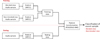 |
Figure 2 Block diagram of the proposed classification model. |
Audio samples were grouped into training and test sets for this blending classification modelling process. The training data, which includes the pre-defined blended and non-blended classes, and test data are then transformed using the chosen feature transformation methods to a low-dimensional feature space, and the distance between clusters is used as a parameter for the blending classification of the test sample. The feature transformation techniques and modelling are explained in Sections 2.2.2 and 2.2.3.
2.1 Preparation of sound samples
A string ensemble consisting of 9 violins was performed at Detmold concert house (Reverb time RT60 = 1.62 s), and the individual instruments were recorded simultaneously using DPA 4099 clip-on microphones attached to each instrument. Two musical pieces (Symphony No. 6 in Bminor, I. Adagio – Allegro non troppo by Tchaikovsky, and Sonata No. 12 in Aflatmajor, II. Scherzo by Beethoven) were sequentially performed in unison by the string ensemble having different numbers of violins (from 1 to 9) and subsequently recorded. The musicians in the ensemble were seated with a separation of roughly 0.8–1 m, and equal gain was applied for all the DPA microphone tracks in the sound card (more details can be found at [7]). DPA 4099 clip-on microphones attached on the instruments were kept close to the violin bridge in order to better capture individual source signals from the joint performance. These microphones have a frequency response of 20 Hz to 20 kHz with an effective frequency range of 80 Hz to 15 kHz (±2 dB) at 20 cm distance. Due to the super-cardioid directivity characteristic of the DPA microphones, the instrument recordings are expected to minimize cross-talk from other instruments and room reflections [21]. These close-miking recordings are assumed to be authentic and intrinsic representatives of realistic musical performances possessing minimal ambient noise and microphone cross-talk, and hence they were utilized in this investigation to obtain sound samples of joint performances.
From these recordings of the 9 violins, 50 sound samples consisting of 2 violin signals were extracted for evaluation. These samples had a duration of approximately 3–5 s each, and they included different musical fragments. The 2 violins in each sample were randomly chosen from the 9 violin tracks, and hence the influence of the coordination effect due to spatial proximity can be assumed to be negligible in the selected samples. The basis of the selection of these samples was that these samples should not provide salient cues for distinguishing the 2 constituent violins such as pitch difference, onset timing asynchrony, etc., and significant noise level from bow & musician. Nevertheless, these 50 samples were differing in terms of blending impressions due to the unavoidable differences in the aforementioned musical factors (see Sect. 1).
The samples were extracted and post-processed in Reaper digital audio workstation; breathing and violin bow noises were minimized using a high pass filter with a cutoff frequency of 200 Hz without attenuating the low notes in the musical pieces. Furthermore, fade-in and fade-out filters of less than 0.3 s duration were added at the beginning and end of the signals. Subsequently, the 2 channels from the violins were rendered by downmixing to a mono-aural sound sample with equal gains on each track at 44.1 kHz/16-bit depth, and these samples were used for the perceptual evaluation.
2.1.1 Perceptual labelling of sound samples
Fourteen musically ear-trained participants including Tonmeister students and professional musicians (4 female, 10 male, mean value of age 28.7 ± 7.2) participated in the listening test. The participants had prior experience in critical listening, and previous studies have shown their sensitivity over non-musicians in selectively attending to and analyzing the complex spectral and temporal features of sounds [22, 23]. So, we expect such a population to better conceive the notion of blending and provide the blending ratings with concordance.
The objective of the listening test and the test procedure were described to the participants at the beginning of the test. The working definition of blending was stated to the participants as “the perceived fusion of violin sounds where the constituent instruments are indistinguishable”. Similar to earlier studies, the blending impression of each sample was rated on a scale from 0 to 10 in which a low value corresponds to poor blending, and a high value corresponds to very good blending. Since the standard examples of the possible extrema of the blending impression between violins are not known, it was not possible to provide the reference samples for the training phase. This might have limited the listeners in conceiving the possible variation in the blending impression in the chosen set of samples and forming their inner-scale of blending rating. Nevertheless, to prime the listener with the sound of the instrument in the DPA microphone recordings, familiarization audio examples consisting of sound samples from the recording were provided at the beginning of the test.
Five audio files, each with 10 sound samples, were generated for the listening test. The sound samples were randomized in the audio files in order to reduce the memory retention effects in ratings. Each sound sample was played three times and the listeners were asked to rate the blending impression of the particular sample on a scale of 0–10 in a test response form. The participants performed the test using studio-grade headphones of their choice in acoustically treated quiet environments. After each audio file, participants had the option to take a short break and resume the test which helped them to reduce mental fatigue. Including short breaks between each set of audio samples, participants took an average of 30 min to complete the test.
Consistency and reliability of listening test rating: When looking at the listening test responses, some of the samples chosen for the study had a high variation in the sample rating, indicating a high inter-participant disparity in the perceived blending impression among the trained participants. This could be due to the different levels of attention given to the musical aspects (e.g., pitch, timbre, onsets, etc.) by the participants while judging the sample. To tackle this problem, and to use sound samples with a considerably consistent rating, a threshold value of standard deviation of 2 was chosen in this study. Accordingly, sound samples with a standard deviation value smaller than 2 were chosen for the classification evaluation which resulted in a final set of 31 sound samples from 50.
The assessment of inter-rater reliability was performed to further evaluate the degree of agreement between the listeners using Cronbach’s alpha [24]. The Cronbach’s alpha value for the selected 31 sound samples was obtained to be 0.93, indicating high reliability among the test participants on the rating of blending.
The probability distribution of the blending ratings of the short-listed 31 sound samples is shown in Figure 3, which demonstrates a bi-modal distribution having 2 maxima around 5.25 and 7.75 and a minimum around 6.5. Based on the bi-modal distribution of blending perception ratings, 2 classes of samples were established – the “blended class” that includes samples with a mean rating > 6.5/10, and the “non-blended class” that includes samples with a mean rating < 6.5/10. Resulting in, the selected sample set having 13 samples from the blended class and 18 samples from the non-blended class.1
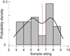 |
Figure 3 Probability distribution of the blending ratings of 31 sound samples (the thick black line shows the probability distribution function; dashed red line indicates the minimum arising between the 2 maxima in the distribution function). |
2.2 Classification modelling
2.2.1 Feature extraction
The Mel Frequency Cepstral Coefficients based subjectively on a nearly logarithmic sense of human auditory pitch perception [26] have been shown to successfully represent perceptually related characteristics of signals [27]. Therefore, they have been used widely in speech signal analysis including speech recognition [27, 28], speaker identification [29], and verification [30]. Other studies further demonstrate their relevance in music modeling [31], musical instrument recognition [32], and voice and musical emotion detection [33, 34], thereby showing performance superior to conventional audio features in MIR applications.
The process of extraction of MFCC features begins with converting the audio signals into frames using a moving time window and performing Discrete Fourier Transformation (DFT) on each frame to get the power spectrum. A filter-bank derived from the Mel scale is then applied to the power spectrum to obtain the Mel-scale power spectrum. The logarithm of the amplitude spectrum is then taken. Finally, a Discrete Cosine Transform (DCT) of the log filter-bank energies generates the Mel Frequency Cepstral Coefficients.
Silent regions at the start and end of the audio samples were removed, and the first 14 MFCCs [35] were extracted for every 100 ms of the audio signal with an overlapping length of 50 ms using a Hamming window. Along with the raw MFCC features, standardized (Z-score normalized) MFCC features were also computed for further analysis due to their applicability in similar related studies [36].
2.2.2 Feature transformation methods
The fundamental purpose of feature transformation using techniques adapted from dimensionality reduction is to project the higher-dimensional data into a lower-dimensional space yet retaining most of the relevant information and removing the redundant or correlated information as well as the undesired noise. It helps in decreasing the complexity of high-dimensional features and also supports in low-dimensional visualization of the features. They have also been shown to improve the performance of the statistical modeling method or machine learning algorithms [37, 38]. Depending on the size, quality, and characteristics of input data (i.e., the feature set), different types of feature transformation algorithms can be used for dimensionality reduction. They can be classified into three main groups — linear vs. non-linear, supervised vs. unsupervised, and random-projection vs. manifold-based [37]. The three feature transformation techniques used in this investigation are detailed below.
Principal Component Analysis (PCA): PCA is a widely used unsupervised and linear dimensionality reduction method. It linearly projects higher-dimensional data into Principal Components (PCs) while maximally preserving input data variance [39]. The principal components are mutually orthogonal and they represent directions of the data that explain a maximal amount of variance.
Estimation of PCs starts by calculating the covariance matrix of the n-dimensional (n = 14 here) input data (X). Next, the Eigenvalue decomposition is done on the covariance matrix to estimate the Eigenvalues and Eigenvectors. A transformation matrix (Wn×k) made up of top k Eigenvectors is used to project X onto a lower-dimensional feature space. The PC transformation minimizes redundancy, noise, and feature collinearity. Non-linear feature extraction techniques outperform the PCA on artificial tasks and can deal with complicated data structures, but studies suggest that they do not outperform PCA in natural data sets [40]. Furthermore, PCA was shown to enhance modeling accuracy and efficiency by transforming MFCCs [28, 32, 41].
Linear Discriminant Analysis (LDA): LDA is a supervised and linear feature transformation technique that uses Fisher’s criterion – maximizing inter-class variance while minimizing intra-class variation – resulting in minimal overlap of features corresponding to different classes (maximum class separation) in new dimensional transformed space [42].
To derive low-dimensional features, 2 scattering matrices are estimated for the predefined classes – (1) within the class scattering matrix (Swc), and (2) between the class scattering matrix (Sbc). The Eigenvalue decomposition is done on the matrix  to derive the Eigenvalues and Eigenvectors. Eigenvectors corresponding to the highest Eigenvalues in the new feature space maximize class separation in the transformed space. Similar to the PCA, a transformation matrix W with the top k Eigenvectors is constructed, which transforms the input data X onto a lower dimension. Unlike PCA, the features in the low dimensional basis are not necessarily orthogonal in LDA [42, 43].
t-Stochastic Neighbourhood Embedding (t-SNE): t-SNE is an unsupervised, non-linear feature transformation that can capture most of the necessary local structure information from a high-dimensional feature space while simultaneously revealing information about the global distribution of the data [44]. In the t-SNE transformation, a probability distribution on pairings in higher dimensions is firstly created by assigning a higher probability to similar objects and a lower value to dissimilar ones. Secondly, the same probability distribution is iteratively replicated on the lower dimension till the Kullback–Leibler divergence is minimized. Euclidean distance was used in this study for the similarity estimation between data points.
2.2.3 Test-train split up and classification criteria
Due to the limited sample size available in our study, implementation of advanced machine learning modelling algorithms like Deep Neural Networks has limitations. Comparison of similarity using distance measures between clusters is a conventional method in statistical modelling [45, 46], and a similar technique is used in this investigation.
The first phase of the modelling process started with randomly dividing the samples into training and testing data sets; in this investigation, we included 23 training and 8 test samples, respectively. The training data included 10 samples from the blended class and 13 samples from the non-blended class, and the test data included 3 samples from the blended class and 5 from the non-blended class. The transformation of the training data (including the pre-defined blended and non-blended classes) and test data to a low-dimensional feature space is performed using the proposed feature transformation methods.
The centroid of the data distribution – the Euclidean coordinate which corresponds to the arithmetic mean of data points across the dimensionality-reduced feature space – is estimated for the blended class, non-blended class, and test data. The Euclidean distance between the centroids of these blended, non-blended classes and the testing audio sample in the low-dimensional feature space was used as the metric for the classification of blending impression. In our classification criteria, if the Euclidean distance between the centroid of the blended class and test data is less than the distance between the centroid of the non-blended class and test data, then the test sample is classified as “blended”, and vice versa. For each test sample, the predicted class from the model was compared with its perceptually labelled class. Accordingly, the performance of each feature transformation technique is estimated.
The results of this evaluation could be biased due to the chosen samples in the training and testing data sets and the limited sample size. To overcome this issue of bias and the possible randomness in the result, the accuracy of the best-performing feature transformation models when evaluated using a distinct training and test set is further validated using Leave-One-Out Cross-Validation (LOOCV). LOOCV involves training the model with all of the data except for one data point, for which a prediction is made. A total of 31 unique models must be trained using 31 data samples; while this is a computationally expensive strategy, it ensures an accurate and unbiased measure of model performance.
3 Results
3.1 Statistical analysis of transformed features
The hypothesis that the distribution of 2 classes (blended and non-blended) in transformed features have equal mean values (null hypothesis) or not was tested using the Mann–Whitney U test [47]. Transformed features corresponding to all 31 samples (13 blended and 18 non-blended) were considered for this analysis. In PCA and LDA, the transformation that preserves maximum data variance (95% in this investigation) was considered. This has resulted in four transformed features for raw MFCC and 9 transformed features for standardized MFCC for PCA transformation, and one transformed feature for both raw and standardized MFCCs for LDA transformation. For t-SNE, the default transformed dimension of three was used for both raw and standardized MFCCs.
PCA feature analysis: The Mann–Whitney U test was performed on the PCA-transformed raw and standardized MFCC features, and the results are shown in Table 1. Additionally, the box plot and probability density function of the 2 classes corresponding to each feature shown in Figures 4 and 5 describe the distribution of PCA-transformed features. Since the distributions of PC7 to PC9 are very similar to those of PC6, they were omitted from Figure 5.
 |
Figure 4 Distribution of PCA-transformed raw MFCC. |
 |
Figure 5 Distribution of PCA-transformed standardized MFCC. |
Mann–Whitney U test summary of the PCA features.
For Mann–Whitney U test results comparing 2 transformed feature sets (see Tab. 1), all p-values (with the exception of PC3 and PC4) are less than 0.05, rejecting the null hypothesis that there is no difference between the mean values of PC1 and PC2 corresponding to the PCA transformed MFCC features of blended and non-blended samples. The exception (p-value greater than 0.05) for the standardized MFCC was PC7.
LDA feature analysis: Mann–Whitney U test result of LDA transformed raw and standardized MFCCs is shown in Table 2 and their distributions are depicted in Figure 6a and 6b, respectively. The p-value of the transformed features corresponding to blended and non-blended samples are less than 0.05, implying that the null hypothesis of equal means is rejected once again. The distribution plots of raw and standardized MFCCs clearly demonstrate the differences between the 2 classes of data and validate the Mann–Whitney U test findings.
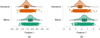 |
Figure 6 Distribution of LDA-transformed (a) raw MFCC, (b) standardized MFCC. |
Mann–Whitney U test result summary of the LDA features.
t-SNE feature analysis: The Mann–Whitney U test findings for t-SNE transformed raw and standardized MFCCs are shown in Table 3, and their respective distributions are illustrated in Figures 7 and 8. The p-value is significant for the second and third t-SNE transformed raw MFCC features, however, the first t-SNE transformed feature is significant for standardized MFCC. Furthermore, the distribution of t-SNE differs from that of PCA and LDA, where notable bimodal characteristics can be detected in the former.
 |
Figure 7 Distribution of t-SNE transformed raw MFCC. |
 |
Figure 8 Distribution of t-SNE transformed standardized MFCC. |
Mann–Whitney U test result summary of the t-SNE features.
3.2 Cluster visualization of PCA, LDA, and t-SNE
Figure 9 shows the cluster distribution of transformed raw MFCC features for blended and non-blended samples. This helps in visualizing the transformation in lower-dimensional space, and the first three transformed features of MFCC were compared across the three transformation techniques. The blended audio features transformed from the training set are represented by red dots, while the non-blended features are represented by green dots. The centroids of blended and non-blended training data distributions are highlighted using red and green spheres. Furthermore, the centroids of the transformed blended audio samples from the test data are shown as red triangles, while that of the non-blended samples are shown as green triangles (see Figs. 9a and 9b). Because the t-SNE transformation matrix is dependent on the test data, the resulting centroid of a non-blended sample (selected as an example) is shown in Figure 9c.
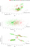 |
Figure 9 Cluster distribution of transformed raw MFCC features for blended and non-blended samples using (a) PCA, (b) LDA, (c) t-SNE. Spheres indicate centroids of blend (red) non-blend (green) training data, while triangles indicate centroids of blend (red) and non-blend (green) test data. |
Because the overall blending rating is considered in this investigation rather than the time varying blending parameter, the 2 classes in training data may overlap, which means that the non-blended sound sample may contain many data points with blended characteristics and vice versa. Looking closely at Figures 9a–9c, the class overlap in PCA, t-SNE, and LDA is visible, though slightly less overlap in the latter. This less overlap could be attributed to the supervised nature of the LDA transformation, which could eventually aid in class identification.
3.3 Classification model result
3.3.1 With separate train-test samples
Table 4 shows the performance of various models for blended-non-blended classification when the model is trained using a fixed training sample set (23 samples) and tested against the remaining eight samples. The table clearly shows that the raw MFCC consistently outperforms the standardized MFCC, which is surprising and contradictory to many previous results on audio classification [48, 49]. Among the six classification models, the transformation of raw MFCC using LDA and subsequent similarity estimation produced the highest accuracy (87.5%). The LDA-supervised transformation, which results in less overlap between the 2 classes (see feature distribution in Fig. 6), could be responsible for this superior performance. PCA and t-SNE transformations of raw MFCCs were relatively worse (75%) as compared to LDA. All the remaining models have resulted in the same accuracy (62.5%). Figure 10 shows the resulting confusion matrices for these models. When using raw MFCC for transformation, LDA misclassified one of the blended signals as non-blended (see Fig. 10c). PCA and t-SNE transformation has an additional non-blended misclassification. The remaining models perform poorly and consistently misclassify blended signals as non-blended.
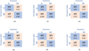 |
Figure 10 Confusion matrices depicting the correct and misclassification rates of the six transformation models trained and validated using separate train and test samples, (number of test samples n = 8). (a) PCA transformed raw MFCC, (b) PCA transformed standardized MFCC, (c) LDA transformed raw MFCC, (d) LDA transformed standardized MFCC, (e) t-SNE transformed raw MFCC and (f) t-SNE transformed standardized MFCC. |
Performance of PCA, LDA and t-SNE transformation models trained and validated using separate train and test samples.
To confirm that the technique selected for feature transformation and classification is free of bias and to assess the likelihood of possible overestimation of accuracy with selected samples from the testing set, a leave-one-out cross-validation technique was finally carried out in this investigation. Although the t-SNE transformation of MFCC exhibits a comparable result to PCA, it can’t be considered to be a generalized solution since the t-SNE transformation is test data-dependent [44]. Further, t-SNE was employed in this study for the completeness of the dimensionality reduction method due to its ability to visualise more sophisticated higher dimensional clustering of data using a non-linear approach. Hence, we limit our LOOCV investigation to the top-performing models from this analysis, i.e., PCA and LDA transformation of raw MFCC. The results of LOOCV are discussed in the following section.
3.3.2 Cross validation of the model
In LOOCV, the model is trained using all of the samples except for one sample, for which a prediction is then made. Table 5 shows the performance of PCA, and LDA transformation models validated using LOOCV, and Figure 11 shows the Confusion matrices depicting correct and misclassification rates in LOOCV (models were trained and validated with 31 separate iterations).
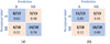 |
Figure 11 Confusion matrices depicting correct and misclassification rates in LOOCV (models were trained and validated with 31 separate iterations). (a) PCA transformed raw MFCC and (b) LDA transformed raw MFCC. |
Performance of PCA and LDA transformation models validated using LOOCV.
LOOCV result is comparable to the earlier result (i.e., from a distinct train-test split). A prediction accuracy of 87.1% for MFCC features transformed using LDA was achieved with 27 correct classifications out of 31. There are 2 misclassifications for both the blended and the non-blended classes. The PCA-transformed MFCC performed marginally worse with 22 correct classifications out of 31. In PCA transformed features, the blended classes misclassified as non-blended are higher than the LDA equivalent (5 out of 13 in PCA compared to 2 out of 13 in LDA). So overall following the result based on the given set of samples, this investigation demonstrates that the MFCC features transformed using Linear Discriminant Analysis are a suitable method for classifying musical score-independent, monophonically rendered dynamic musical signals in terms of their overall perception of the source-level blending impression.
4 Discussion
This study used a computational approach to classify monophonic recordings of unison performances by 2 violins into blended or non-blended classes based on their overall impression of source-level blending, while the 2 latter classes were perceptually validated through a listening experiment with expert listeners. The classification accuracy reached up to 87%, indicating a promising method that considered realistic sound samples with different musical content without accessing individual source recordings. Our study shows that a computational approach can model certain aspects of complex psychoacoustic phenomena such as musical blending, and thus introduces a new tactic to address a stubborn and difficult auditory puzzle. In this regard, this study differs from earlier studies on understanding and assessing blending in that it directly incorporated “ecologically” realistic sound samples containing musical excerpts representing diverse musical contents, and was not restricted only to musical notes or chords [3, 9, 10]. Given that this ecologically representative approach has never been attempted before increases the novelty and impact of our study. Moreover, we advanced the state-of-the-art by incorporating methods from the disciplines of Music Information Retrieval (MIR) and Machine Learning in this music perception-related research problem.
Unfortunately, a direct comparison of this study with earlier investigations that treated blending as a continuous variable is not possible since this study performed the binary classification of sound samples into blended and non-blended classes. Further, while rating sound samples that contained musical excerpts, only a single-valued rating that represents the “overall” impression of blending was given for each sample, which was not finely resolved in time. Hence, we acknowledge this subjective rating may not always be useful in explaining the temporally continuous variation of musical attributes in other contexts (e.g. a short performance mistake that occurred for 100 ms in a highly blended sample may have a stronger effect on its final overall impression of the blend for the whole sample). Nevertheless, we observed the bi-modal probability distribution of sample ratings (see Fig. 3), therefore the naive classification of the samples into 2 categories is not unreasonable.
The notion and perception of musical blending can differ across individuals from a heterogeneous background, thus this feasibility study was performed “only” among musically ear-trained critical listeners (who are expected to be sensitive and perceptive to audio cues and hence offer good convergence in terms of the musical agreement), and thereby expected to reduce variance and inconsistencies in perceptual labeling. Additionally, in contrast to previous studies which employed instrument recordings from sophisticated recording conditions [9, 10], this study utilized in-situ recordings of an ensemble performance from a concert hall which was carried out by intentionally not restricting the natural environment of the musicians and the auditory and visual feedback from the performers and acoustic space, and thus represents an “ecological” musical and listening context. Therefore, unlike the necessity of having “acoustically clean” signals, this study made use of authentic and natural representative sound samples of joint musical performance having natural ambient noise and negligible microphone crosstalk – this increased representativeness of natural musical performance thus broadens the relevance when studying other in-situ joint musical performances.
Although MFCCs are widely used in Music Information Retrieval (MIR) to describe spectral and timbre information [50], we note that the coefficients alone offer limited insight into music perception [51] and by extension, limited utility to explain blending impression in terms of temporal, spectral, and energy-based musical attributes. In our approach, we did not incorporate certain prominent feature parameters from time and frequency domains that were explored in earlier blending studies [3, 9, 10] such as pitch, spectral centroid, attack contrast, and loudness correlation, etc. The reason for not using them in our approach is that our study focuses on monophonically rendered audio samples, while those parameters were specifically designed for individual source channels. Since this work is limited to MFCC features, alternative MIR features would be studied and included in future studies for modelling the blending perception.
By performing a 2-fold evaluation (test-train split up, and cross-validation), we have also checked for bias or chance predictions arising from the proposed classification model. Having developed the blending classification model, we now have a tool that allows future work to focus on the estimation of blending impressions of dynamic music samples using large and diverse datasets (that includes samples having different numbers and combinations of instruments, or samples manipulated to explore audio features like pitch, spectral centroid, onset time, loudness, etc.,) and also further extending the modelling to machine learning models such as decision trees, Support Vector machines (SVM), Neural Networks, etc. The final goal would be to finally comprehensively assess the blending of sound sources as a time-varying parameter by also incorporating room acoustic contribution.
5 Conclusion
This investigation demonstrates the feasibility of classifying musically realistic sound samples based on their overall blending impression perceived between 2 musical instruments in a unison performance. Musical score-independent monophonically rendered sound samples extracted from in-situ recordings of an ensemble performance were used for the perceptual evaluation of blending impressions and the corresponding classification modelling. The results show that the Linear Discriminant Analysis paired with the Euclidean distance measure performed on the raw MFCC features extracted from the sound samples is an effective method of classifying these sound samples into blended and non-blended classes. The model was tested and verified using a separate train-test data set, and leave-one-out cross-validation which showed an accuracy of 87.5%, and 87.1% respectively. This outperforms the other models tested in this study which were developed using the PCA and t-SNE transformations of raw and standardized MFCC features. Unlike the previous research on the estimation of source-level blending impression which employed musically constrained sound samples (such as notes or chords) of instruments from sophisticated recording conditions, this study surpasses earlier limitations by implementing the classification of “ecological” sound samples of joint performances even without accessing the individual source recordings.
This investigation serves as a proof of concept for the capability of feature transformations to categorize the perception of multivariate psychoacoustic blending phenomenon, despite the fact that the perceptual rating scale is subjective and may vary depending on the listeners’ backgrounds and the characteristics of the audio samples. The proposed method could be further expanded using a larger sample size and applied in various domains such as joint musical performance training, and real and virtual orchestral sound evaluation because it is independent of the musical content of the signal and does not require access to the individual source signals. Given that the method is applicable for sound signals from joint performance recording with minimal microphone cross-talk and background noise, this expands its utility in in-situ applications.
Conflict of interest
Author declared no conflict of interests.
Data availability statement
The sound samples associated with this article and the cluster distribution plots (Fig. 9) are available in Zenodo under the reference [25]. The data uploaded to the Zenodo repository are under the scientific responsibility of the authors.
Acknowledgments
The authors thank the musicians and listening test participants for their kind cooperation. Thanks to Boris Alex Bolles and Stefanos Ioannou for their support in recording the string Ensemble. The authors acknowledge the ODESSA project participants, a collaborative project in the context of the ACTOR project, for the planning of the ODESSA-III recording.
Funding
This work has been performed within the project VRACE (Virtual Reality Audio for Cyber Environments) which has received funding from the European Union’s Horizon 2020 research and innovation program under the Marie Sklodowska Curie actions (grant agreement number 812719).
The selected sound samples are available at [25].
References
- A.W. Goodwin: An acoustical study of individual voices in choral blend. Journal of Research in Music Education 28, 2 (1980) 119–128. [CrossRef] [Google Scholar]
- R.A. Kendall, E.C. Carterette: Identification and blend of timbres as a basis for orchestration. Contemporary Music Review 9, 1–2 (1993) 51–67. [CrossRef] [Google Scholar]
- G.J. Sandell: Roles for spectral centroid and other factors in determining “blended” instrument pairings in orchestration. Music Perception 13, 2 (1995) 209–246. [CrossRef] [Google Scholar]
- S.A. Lembke, S. Levine, S. Mcadams: Blending between bassoon and horn players: An analysis of timbral adjustments during musical performance. Music Perception: An Interdisciplinary Journal 35 (2017) 144–164. [CrossRef] [Google Scholar]
- M. De Francisco, M. Kob, J.F. Rivest, C. Traube: ODESSA – orchestral distribution effects in sound, space and acoustics: an interdisciplinary symphonic recording for the study of orchestral sound blending, in: Proceedings of International Symposium on Musical Acoustics (ISMA), 13–17 November 2019, Detmold, Germany, 2019, pp. 33–41. [Google Scholar]
- S. Ioannou, M. Kob: Investigation of the blending of sound in a string ensemble, in: Proceedings of International Symposium on Musical Acoustics (ISMA), 13–17 November 2019, Detmold, Germany, 2019, pp. 42–49. [Google Scholar]
- J. Thilakan, M. Kob: Evaluation of subjective impression of instrument blending in a string ensemble, in: Fortschritte der Akustik – DAGA 2021, 15–18 August 2021, Vienna, Austria, 2021, pp. 524–527. [Google Scholar]
- J. Thilakan, O.C. Gomes, M. Kob: The influence of room acoustic parameters on the impression of orchestral blending, in: Proceedings of Euronoise 2021, 25–27 October 2021, Madeira, Portugal/Online, 2021. [Google Scholar]
- S.A. Lembke, S. Mcadams: The role of spectral-envelope characteristics in perceptual blending of wind-instrument sounds. Acta Acustica united with Acustica 101, 5 (2015) 1039–1051. [CrossRef] [Google Scholar]
- S.A. Lembke, K. Parker, E. Narmour, S. Mcadams: Acoustical correlates of perceptual blend in timbre dyads and triads. Musicae Scientiae 23, 2 (2019) 250–274. [CrossRef] [Google Scholar]
- A.S. Bregman: Auditory scene analysis: the perceptual organization of sound, The MIT Press, Cambridge MA, 1990. [CrossRef] [Google Scholar]
- S. Ternström: Preferred self-to-other ratios in choir singing. Journal of the Acoustical Society of America 105, 6 (1999) 3563–3574. [CrossRef] [PubMed] [Google Scholar]
- J. Daugherty: Choir spacing and formation: choral sound preferences in random, synergistic, and gender-specific chamber choir placements. International Journal of Research in Choral Singing 1, 1 (2003) 48–59. [Google Scholar]
- W. Goebl, C. Palmer: Synchronization of timing and motion among performing musicians. Music Perception 26, 5 (2009) 427–438. [CrossRef] [Google Scholar]
- S. Bolzinger, O. Warusfel, E. Kahle: A study of the influence of room acoustics on piano performance. Le Journal de Physique IV 4, C5 (1994) 617–620. [Google Scholar]
- Z.S. Kalkandjiev, S. Weinzierl: The influence of room acoustics on solo music performance: an experimental study. Psychomusicology: Music, Mind and Brain 25, 3 (2015) 195–207. [CrossRef] [Google Scholar]
- S.V.A. Garí, M. Kob, T. Lokki: Analysis of trumpet performance adjustments due to room acoustics, in: Proceedings of International Symposium on Room Acoustics (ISRA) 2019, 15–17 September 2019, Amsterdam, Netherlands, 2019. [Google Scholar]
- P.F. Assmann, Q. Summerfield: Modeling the perception of concurrent vowels: vowels with different fundamental frequencies. Journal of the Acoustical Society of America 88, 2 (1990) 680–697. [CrossRef] [PubMed] [Google Scholar]
- A. de Cheveigné, H. Kawahara, M. Tsuzaki, K. Aikawa: Concurrent vowel identification. I. Effects of relative amplitude and F0 difference. Journal of the Acoustical Society of America 101, 5 (1997) 2839–2847. [CrossRef] [Google Scholar]
- R.A. Rasch: Synchronization in performed ensemble music. Acustica 43, 2 (1979) 121–131. [Google Scholar]
- https://www.dpamicrophones.com/instrument/4099-instrument-microphone. [Google Scholar]
- D.R. Soderquist: Frequency analysis and the critical band. Psychonomic Science 21, 2 (1970) 117–119. [CrossRef] [Google Scholar]
- B.C.J. Moore: An introduction to the psychology of hearing, Elsevier Ltd, London, 2004. [Google Scholar]
- L.J. Cronbach: Coefficient alpha and the internal structure of tests. Psychometrika 16, 3 (1951) 297–334. [CrossRef] [Google Scholar]
- J. Thilakan, B. BT, J. Chen, M. Kob: Sound samples for the evaluation of source-level blending between violins (Version 1.1) [Audio data set]. Zenodo. Available at: https://doi.org/10.5281/zenodo.8278236. [Google Scholar]
- S.S. Stevens, J. Volkmann, E.B. Newman: A scale for the measurement of the psychological magnitude pitch. Journal of the Acoustical Society of America 8, 3 (1937) 185–190. [CrossRef] [Google Scholar]
- S. Davis, P. Mermelstein: Comparison of parametric representations for monosyllabic word recognition in continuously spoken sentences. IEEE Transactions on Acoustics, Speech and Signal Processing 28 (1980) 357–366. [CrossRef] [Google Scholar]
- A. Winursito, R. Hidayat, A. Bejo: Improvement of MFCC feature extraction accuracy using PCA in Indonesian speech recognition, in: International Conference on Information and Communications Technology (ICOIACT), IEEE, 2018, pp. 379–383. [Google Scholar]
- L. Muda, M. Begam, I. Elamvazuthi: Voice recognition algorithms using Mel frequency cepstral coefficient (MFCC) and dynamic timewarping (DTW) techniques, 2010. arxiv:1003.4083. [Google Scholar]
- S.H. Chen, Y.R. Luo: Speaker verification using MFCC and support vector machine, in: Proceedings of the International MultiConference of Engineers and Computer Scientists (IMECS) 2009, vol. 1, 18–20 March 2009, Hong Kong, 2009, pp. 18–20. [Google Scholar]
- B. Logan: Mel frequency cepstral coefficients for music modeling, in: Proceedings of International Symposium on Music Information Retrieval (Music IR) 2000, vol. 270, no. 1, 23–25 October 2000, Massachusetts, USA, 2000. [Google Scholar]
- R. Loughran, J. Walker, M. O’Neill, M. O’Farrell: The use of Mel-frequency cepstral coefficients in musical instrument identification, in: Proceedings of International Computer Music Conference Proceedings (ICMA) 2008, 24–29 August 2008, Belfast, Ireland, 2008. [Google Scholar]
- M. Gilke, P. Kachare, R. Kothalikar, V.P. Rodrigues, M. Pednekar. MFCC-based vocal emotion recognition using ANN, in: Proceedings of International Conference on Electronics Engineering and Informatics (ICEEI) 2012, vol. 49, 1–2 September 2012, Phuket, Thailand, 2012, pp. 150–154. [Google Scholar]
- S. Rajesh, N.J. Nalini: Musical instrument emotion recognition using deep recurrent neural network. Procedia Computer Science 167 (2020) 16–25. [CrossRef] [Google Scholar]
- A.B. Kandali, A. Routray, T.K. Basu: Emotion recognition from Assamese speeches using MFCC features and GMM classifier, in: TENCON 2008–2008 IEEE Region 10 Conference, IEEE, 2008, pp. 1–5. [Google Scholar]
- C. Richter, N.H, Feldman, H. Salgado, A. Jansen: A framework for evaluating speech representations, in: Proceedings of the Annual Conference of the Cognitive Science Society, 2016. [Google Scholar]
- F. Anowar, S. Sadaoui, B. Selim: Conceptual and empirical comparison of dimensionality reduction algorithms (PCA, KPCA, LDA, MDS, SVD, LLE, ISOMAP, LE, ICA, t-SNE). Computer Science Review 40 (2021) 100378. [CrossRef] [Google Scholar]
- S. Dupont, T. Ravet, C. Picard-Limpens, C. Frisson: Nonlinear dimensionality reduction approaches applied to music and textural sounds, in: Proceedings of International Conference on Multimedia and Expo (ICME), IEEE, 2013, 1–6. [Google Scholar]
- H. Hotelling: Analysis of a complex of statistical variables into principal components. Journal of Educational Psychology 24, 6 (1933) 417. [CrossRef] [Google Scholar]
- L. Van Der Maaten, E.O. Postma, H.J. Van den Herik: Dimensionality reduction: a comparative review. Journal of Machine Learning Research 10 (2009) 66–71. [Google Scholar]
- C. Ittichaichareon, S. Suksri, T. Yingthawornsuk: Speech recognition using MFCC, in: Proceedings of International Conference on Computer Graphics, Simulation and Modeling (ICGSM) 2012, vol. 9, 28–29 July 2012, Pattaya, Thailand, 2012. [Google Scholar]
- A. Tharwat, T. Gaber, A. Ibrahim, A.E. Hassanien: Linear discriminant analysis: a detailed tutorial. AI Communications 30, 2 (2017) 169–190. [CrossRef] [Google Scholar]
- J. Ye, T. Xiong, D. Madigan: Computational and theoretical analysis of null space and orthogonal linear discriminant analysis. Journal of Machine Learning Research 7, 7 (2006) 1183–1204. [Google Scholar]
- L. Van Der Maaten, G. Hinton: Visualizing data using t-SNE. Journal of Machine Learning Research 9 (2008) 2579–2605. [Google Scholar]
- K.L. Elmore, M.B. Richman. Euclidean distance as a similarity metric for principal component analysis. Monthly Weather Review 129, 3 (2001) 540–549. [CrossRef] [Google Scholar]
- M.K. Singh, N. Singh, A.K. Singh: Speaker’s voice characteristics and similarity measurement using Euclidean distances, in: Proceedings of International Conference on Signal Processing and Communication (ICSC), IEEE, 2019, pp. 317–322. [Google Scholar]
- H.B. Mann, D.R. Whitney: On a test of whether one of two random variables is stochastically larger than the other. Annals of Mathematical Statistics 18, 1 (1947) 50–60. [Google Scholar]
- D. Perna, A. Tagarelli: Deep auscultation: predicting respiratory anomalies and diseases via recurrent neural networks, in: Proceedings of 32nd International Symposium on Computer-Based Medical Systems (CBMS), IEEE, 2019. [Google Scholar]
- S.F. Chang, D. Ellis, W. Jiang, K. Lee, A. Yanagawa, A.C. Loui, J. Luo: Large-scale multimodal semantic concept detection for consumer video, in: Proceedings of the 9th ACM SIGMM International Workshop on Workshop on Multimedia Information Retrieval (MIR 2007), 24–29 September 2007, Bavaria, Germany, 2007, pp. 255–264. [Google Scholar]
- H. Terasawa, J. Berger, S. Makino: In search of a perceptual metric for timbre: dissimilarity judgments among synthetic sounds with MFCC-derived spectral envelopes. Journal of the Audio Engineering Society 60, 9 (2012) 674–685. [Google Scholar]
- K. Siedenburg, I. Fujinaga, S. McAdams: A comparison of approaches to timbre descriptors in music information retrieval and music psychology. Journal of New Music Research 45, 1 (2016) 27–41. [CrossRef] [Google Scholar]
Cite this article as: Thilakan J. BT Balamurali Chen J-M. & Kob M.. 2023. Classification of the perceptual impression of sourcelevel blending between violins in a joint performance. Acta Acustica, 7, 62.
All Tables
Performance of PCA, LDA and t-SNE transformation models trained and validated using separate train and test samples.
All Figures
 |
Figure 1 Acoustic path of ensemble sound formation and information, based on [8]. |
| In the text | |
|
Figure 2 Block diagram of the proposed classification model. |
| In the text | |
|
Figure 3 Probability distribution of the blending ratings of 31 sound samples (the thick black line shows the probability distribution function; dashed red line indicates the minimum arising between the 2 maxima in the distribution function). |
| In the text | |
|
Figure 4 Distribution of PCA-transformed raw MFCC. |
| In the text | |
|
Figure 5 Distribution of PCA-transformed standardized MFCC. |
| In the text | |
|
Figure 6 Distribution of LDA-transformed (a) raw MFCC, (b) standardized MFCC. |
| In the text | |
|
Figure 7 Distribution of t-SNE transformed raw MFCC. |
| In the text | |
|
Figure 8 Distribution of t-SNE transformed standardized MFCC. |
| In the text | |
|
Figure 9 Cluster distribution of transformed raw MFCC features for blended and non-blended samples using (a) PCA, (b) LDA, (c) t-SNE. Spheres indicate centroids of blend (red) non-blend (green) training data, while triangles indicate centroids of blend (red) and non-blend (green) test data. |
| In the text | |
|
Figure 10 Confusion matrices depicting the correct and misclassification rates of the six transformation models trained and validated using separate train and test samples, (number of test samples n = 8). (a) PCA transformed raw MFCC, (b) PCA transformed standardized MFCC, (c) LDA transformed raw MFCC, (d) LDA transformed standardized MFCC, (e) t-SNE transformed raw MFCC and (f) t-SNE transformed standardized MFCC. |
| In the text | |
|
Figure 11 Confusion matrices depicting correct and misclassification rates in LOOCV (models were trained and validated with 31 separate iterations). (a) PCA transformed raw MFCC and (b) LDA transformed raw MFCC. |
| In the text | |
Current usage metrics show cumulative count of Article Views (full-text article views including HTML views, PDF and ePub downloads, according to the available data) and Abstracts Views on Vision4Press platform.
Data correspond to usage on the plateform after 2015. The current usage metrics is available 48-96 hours after online publication and is updated daily on week days.
Initial download of the metrics may take a while.