© The Author(s), Published by EDP Sciences, 2025

1 Introduction

Improvement in the acoustic performances of maritime vessels, such as submarines [1, 2], pipeline systems [3, 4] and autonomous underwater vehicles, rely on vibroacoustics simulations. Therefore, efficient numerical modeling of relevant underwater vibroacoustic systems underpins ocean engineering applications. The finite element method (FEM) has been an important numerical method in resolving such systems. However, the application of FEM necessitates careful meshing and mesh resolution that scales with higher frequencies resulting in computational inefficiencies. Such analysis is then limited to the low frequency. Sub-structuring is then introduced as a means to circumvent the issues of sizable models. The premise of sub-structuring involves decomposing the target system into smaller subsystems that are analyzed individually. Transfer functions can be determined based on coupling and decoupling principles to re-assemble the target system based on the analysis of the simpler subsystems. The advantage is that the subsystems possess simpler geometries which enable improved computational performance with FEM, and in some circumstances, an analytical solution may be available, making the computation significantly efficient.

Early sub-structuring techniques involved coupling with the so-called admittance approach, where admittance is a transfer function defined as a ratio between velocity and force for an element on the structure. Its origin is presented in a work by Gardonio and Brennan [5]. The target system is analyzed as subsystems that are coupled to each other by transfer functions based on the mechanical continuity at the coupling lines. The modal characteristics of ring-stiffened cylindrical shells were analyzed with the admittance approach by Wilken and Soedel [6], which can be recognized to be relevant in maritime engineering applications. As a special case to the admittance approach, the circumferential admittance approach (CAA) was developed by Maxit [7], in which the formulation is tailored to axisymmetric line coupled systems. An extension of the admittance approach was then introduced by Ouisse et al. [8], known as the patch transfer function (PTF) approach. The PTF approach was developed to couple surfaces rather than points. This scheme involves discretizing the coupling surfaces into elementary surfaces known as patches, which together form a transfer matrix. Studies have been focused on both automotive systems [9] and in complex vibroacoustic environments [10]. In recent works, a generalization of the previous approaches was developed by Meyer et al. [11, 12], namely, the condensed transfer function (CTF) approach. Its formulation enables the coupling of subsystems along lines or surfaces. Therefore, the PTF approach is a special case of the CTF approach. The CTF approach was subsequently applied in the analysis of stiffened fluid-loaded cylindrical shells to predict its acoustic radiation [11] and scattering [12]. Additionally, its reverse formulation (i.e., decoupling scheme), known as the reverse condensed transfer function (rCTF) approach, was recently developed [13]. Noticeably, the study of a partially coated cylindrical shell was presented [14], in which a portion of the coating is decoupled from the fluid-loaded cylindrical shell as a demonstration of the subtractive aspect of rCTF. Together with its coupling counterpart, the CTF-rCTF provides a generalized approach to solving complex vibroacoustic analysis.

It is recognized that underwater vibroacoustic systems are typically involved in an acoustic free field (deep oceans). However, the influence of acoustic boundaries such as the sea surface and seabed significantly alters the vibroacoustic behaviour of underwater structures (see for examples, Refs. [15–17]). Relevant to ocean engineering is the shallow water environment, which can be represented as a fluid domain of a perfect underwater waveguide. This refers to a rigid floor to represent the seabed. The sea surface is represented by a free surface. Therefore, this investigation aims to present a preliminary study to showcase the potential of CTF-rCTF in its novel application of a cylindrical shell in a perfect underwater waveguide. As previously mentioned, the problem of complex geometry has been tackled by CTF [11, 12], and in missing coating with rCTF [14]. The novelty of this work is in applying the CTF-rCTF sub-structuring technique to a vibroacoustic system in which the fluid domain is made relatively complex by the involvement of acoustic boundaries. Contrary to an unbounded domain considered in the previous studies, this acoustic domain exhibits a more complex behavior (in particular, standing waves in the vertical direction can appear at specific frequencies). Particular attention will be given to the strong fluid-structure interaction as the decoupling boundary is located at the interface between the structure and the surrounding fluid. The system of interest involves an infinitely-long cylindrical shell under harmonic line excitation and immersed in a fluid domain of a perfect underwater waveguide. Recently, an analytical solution has been provided [18] and will be used as a reference to validate the accuracy of the predictions made using CTF-rCTF. This work, therefore, asserts the possibility of future investigations of complex structures immersed in complex fluid domains, made efficient by the use of CTF-rCTF. It must be underlined that the main objective of this paper is to be able to reproduce the results of reference [18] using the coupled CTF-rCTF approach. Even if this is not the most straightforward way to tackle the considered problem, the versatility of the CTF-rCTF approach allows considering the perspective of applying it on a three-dimensional system with a finite cylindrical shell, contrary to the analytical formulation derived in [18]. Contrary to a full scale 3-D FE model, the addition of internal structures to the model of the cylindrical shell such as stiffeners or bulckheads would not add much complexity to the calculation (as it was already done using CTF approach in references [19] and [20]. Besides, in this paper, the potential of the coupled CTF-rCTF approach is strengthened in the sense that it deals with purely acoustical and mechanical subsystems to subsequently study a coupled vibroacoustic system, highlighting the novelty of the approach.

A comprehensive outline of the theoretical formulation necessary to applying the CTF-rCTF procedure to the system of interest is proposed in Section 2. For more details on the fundamentals of these approaches, it is recommended to refer to Ref. [13]. Results are then presented in Section 3. The analysis is presented for two types of condensation functions used to define the condensed transfer functions as well as two partitions of the global system. Finally, concluding remarks and recommendations for possible future works are described in Section 4.

2 Subtractive modeling applied to a shell immersed in a waveguide

2.1 Presentation of the model and the coupling/decoupling procedure

The system of interest involves an infinitely long cylindrical shell of thickness h_s, radius R, Young’s modulus E_s, Poisson’s ratio ν and density ρ_s, immersed in an acoustic waveguide filled by a heavy fluid of density ρ_f and sound speed c_f, as shown in Figure 1. The waveguide is closed on its upper boundary by a free surface, that is modeled by a pressure release boundary condition, and on its lower boundary by a rigid floor. The total depth of the waveguide is H, where the distance from the origin to the free surface is H_fs, and the distance from the origin to the rigid floor is H_sb. The origin is the center of the shell.

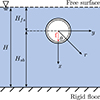Figure 1 Cylindrical shell in a perfect acoustic waveguide.

The shell is excited by a harmonic line force f along the z direction at an angle θ₀ from the x axis. The system is described by cylindrical coordinates (r, θ, z). As the system is uniform along the z-coordinate, it can be reduced to a 2-D problem where the shell is excited by a mechanical point force at the coordinate z = 0.

Two steps are required to study this problem with sub-structuring, as illustrated in Figure 2. The first step, as shown in Figure 2a, called the decoupling procedure, involves removing a disk of fluid (subsystem 2) from a perfect acoustic waveguide (system 1+2). The disk of fluid must occupy the water volume that will ultimately be filled by the cylindrical shell. This step can be performed using the rCTF approach [13]. It results in an intermediary subsystem consisting of the perfect acoustic waveguide with a rigid disk replacing the initial water disk (subsystem 1). In the second step, the excited shell (subsystem 3) is then recoupled using the CTF method [11], as illustrated in Figure 2b.

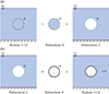Figure 2 (a) Decoupling procedure. (b) Recoupling procedure.

2.2 Theoretical formulation

2.2.1 Definition of the condensed transfer functions

In this section, the definition of the Condensed Transfer Functions (CTFs) used in the CTF and rCTF approaches is reminded. Two systems coupled along a boundary Ω are considered. A set of N orthonormal functions, called condensation functions, is defined on Ω: {φ^ζ}_1≤ζ≤N. For each system α, the pressures p_α and normal velocities u_α on Ω can be expressed as a linear combination of the condensation functions

$$\{\begin{array}{l}{p}_{\alpha }\left(\theta \right)\simeq \sum _{\zeta =1}^N\mathrm{}{P}_{\alpha }^{\zeta }{\phi }^{\zeta }\left(\theta \right)\\ u_{\alpha }\left(\theta \right)\simeq \sum _{\zeta =1}^N\mathrm{}{U}_{\alpha }^{\zeta }{\phi }^{\zeta }\left(\theta \right)\end{array}, \theta \in \mathrm{\Omega },$$(1)

where $P_{\alpha }^{\zeta }$ and $U_{\alpha }^{\zeta }$ are unknowns which will be estimated by the CTF-rCTF approach.

The CTFs are defined based on the nature of the subsystem (acoustic or mechanical) and the decoupling or coupling boundary Ω (tangible or fictitious):

• As system 1+2 is an acoustic system with a fictitious decoupling boundary, the CTFs are defined by prescribing a velocity jump δu₁₊₂ = φ^ξ on Ω, meaning that the CTFs will result in condensed impedances [13, 21]

$$Z_{1+2}^{\zeta \xi }=\frac{P_{1+2}^{\zeta }}{\delta U_{1+2}^{\xi }}=\frac{\langle {\overline{p}}_{1+2},{\phi }^{\zeta }\rangle }{\langle \delta u_{1+2},{\phi }^{\xi }\rangle }=\langle {\overline{p}}_{1+2},{\phi }^{\zeta }\rangle ,$$(2)

where $\langle f,g\rangle ={\int }_{\mathrm{\Omega }}\mathrm{}f\left(\mathbf{x}\right)g^{\mathrm{*}}\left(\mathbf{x}\right)\mathbf{x}$ (with * denoting the complex conjugate and x a point of coordinates (x,y)), and ${\overline{p}}_{1+2}$ corresponds to the resulting pressure on Ω when the system is excited by δu₁₊₂ = φ^ξ.

• Subsystems 1 and 2 are acoustic subsystems with a tangible boundary Ω. The CTFs are then defined by applying a prescribed velocity u_α = φ^ξ on Ω, meaning that the CTFs will result in condensed impedances

$$Z_{\alpha }^{\zeta \xi }=\frac{P_{\alpha }^{\zeta }}{U_{\alpha }^{\xi }}=\frac{\langle {\overline{p}}_{\alpha },{\phi }^{\zeta }\rangle }{\langle u_{\alpha },{\phi }^{\xi }\rangle }=\langle {\overline{p}}_2,{\phi }^{\zeta }\rangle ,$$(3)

with α = 1 or 2.

• Subsystem 3 is a mechanical subsystem with a tangible boundary. Hence the CTFs are defined by applying a mechanical pressure p₃ = φ^ξ on Ω, meaning that the CTFs will result in condensed admittances

$$Y_3^{\zeta \xi }=\frac{U_3^{\zeta }}{P_3^{\xi }}=\frac{\langle {\overline{u}}_3,{\phi }^{\zeta }\rangle }{\langle p_3,{\phi }^{\xi }\rangle }=\langle {\overline{u}}_3,{\phi }^{\zeta }\rangle ,$$(4)

where ${\overline{u}}_3$ corresponds to the normal velocity on Ω when the system is excited by p₃ = φ^ξ. For all of the involved (sub)systems, the condensed transfer functions are calculated for each couple of condensation functions, subsequently defining the matrix as ${\mathbf{X}}_{\mathbf{\alpha }}={\left[X_{\alpha }^{\zeta \xi }\right]}_{N\times N}$, with X being either Y or Z.

As stated above, the problem is solved in two steps: the decoupling and the recoupling procedures. The aim of the decoupling procedure is to obtain quantities related to subsystem 1 (i.e., the waveguide with a rigid disk). Then, the quantities obtained from the decoupling procedure are reinjected into the equations of the CTF method (i.e., the recoupling procedure) to obtain the final quantity, which is the pressure radiated in the waveguide. Those developments will be presented hereafter in reverse order: the recoupling procedure will be addressed first as though the quantities related to subsystem 1 are known. This will highlight the quantities that must be derived from the decoupling procedure, which will be subsequently addressed.

2.2.2 Recoupling procedure

In the recoupling procedure, two subsystems are considered: the waveguide with a rigid disk (subsystem 1), and the uncoupled cylindrical shell excited by a mechanical force (subsystem 3), as illustrated in Figure 2b. Subsystem 1 is an acoustic subsystem, so the condensed impedances of this subsystem can be expressed according to equation (3), and is only subjected to the coupling forces at the boundary Ω. Subsystem 3 is a mechanical system, and its condensed admittances are defined by equation (4). It is subjected to the coupling forces at the boundary Ω and to the external mechanical point force. In response to these coupling forces and the external force, the superposition principle for linear passive systems [11] allows expressing the condensed velocity and pressure vectors on Ω as

$$\{\begin{array}{l}{\mathbf{P}}_{\mathbf{1}}={\mathbf{Z}}_{\mathbf{1}}{\mathbf{U}}_{\mathbf{1}},\\ {\mathbf{U}}_{\mathbf{3}}={\tilde{\mathbf{U}}}_{\mathbf{3}}+{\mathbf{Y}}_{\mathbf{3}}{\mathbf{P}}_{\mathbf{3}}.\end{array}$$(5)

It is worth mentioning that the quantities P_α and U_α are condensed pressure and condensed velocity vectors respectively, and are defined as ${\mathbf{\Gamma }}_{\mathbf{\alpha }}={\left[{\mathrm{\Gamma }}_{\alpha }^{\zeta }\right]}_{N\times 1}$, with Γ being either P or U. ${\tilde{\mathbf{U}}}_{\mathbf{3}}$ (i.e., ${\tilde{U}}_3^{\zeta }=\langle {\tilde{u}}_3,{\phi }^{\zeta }\rangle$, where ${\tilde{u}}_3$ is the shell displacement on Ω when the shell is excited by the external force) is then the vector of the free condensed velocities of subsystem 3 associated with the external mechanical force. The continuity conditions at the coupling boundary Ω and the projection of those conditions on the condensation functions reads

$$\{\begin{array}{l}{\mathbf{P}}_{\mathbf{1}}={\mathbf{P}}_{\mathbf{3}},\\ {\mathbf{U}}_{\mathbf{1}}={\mathbf{U}}_{\mathbf{3}}.\end{array}$$(6)

Then, the combination of equations (5) and (6) allows deducing the coupling condensed velocities between the two subsystems, U₁₊₃ (i.e., U₁₊₃ = U₁ = U₃)

$${\mathbf{U}}_{\mathbf{1}+\mathbf{3}}={\left(\mathbf{I}-{\mathbf{Y}}_{\mathbf{3}}{\mathbf{Z}}_{\mathbf{1}}\right)}^{-1}{\tilde{\mathbf{U}}}_{\mathbf{3}}.$$(7)

Finally, the pressure radiated in the waveguide can be calculated from the knowledge of the coupling velocity as being

$$p_{1+3}\left(M_1\right)={\left({\mathbf{Z}}_{\mathbf{1}}^{{\mathbf{M}}_{\mathbf{1}}}\right)}^T{\left(\mathbf{I}-{\mathbf{Y}}_{\mathbf{3}}{\mathbf{Z}}_{\mathbf{1}}\right)}^{-1}{\tilde{\mathbf{U}}}_{\mathbf{3}}.$$(8)

where I is the identity matrix and ${\mathbf{Z}}_{\mathbf{1}}^{{\mathbf{M}}_{\mathbf{1}}}$ is the vector of the point condensed impedances of subsystem 1. The component ζ of this vector corresponds to the pressure at point M₁ in the uncoupled subsystem 1 when Ω is excited by the condensation function φ^ζ. Following those developments, it appears that the two quantities related to subsystem 1, which must be obtained from the decoupling process, are Z₁ and ${\mathbf{Z}}_{\mathbf{1}}^{{\mathbf{M}}_{\mathbf{1}}}$. The procedure to obtain those quantities using the rCTF method will be described in the next paragraph.

Similarly, the vibration of the shell can be inferred from equations (5) and (7) at any point M₃, initially belonging to subsystem 3

$$u_{1+3}\left(M_3\right)={\tilde{u}}_3\left(M_3\right)+{\left({\mathbf{Y}}_{\mathbf{3}}^{{\mathbf{M}}_{\mathbf{3}}}\right)}^T{\mathbf{Z}}_{\mathbf{1}}{\left(\mathbf{I}-{\mathbf{Y}}_{\mathbf{3}}{\mathbf{Z}}_{\mathbf{1}}\right)}^{-1}{\tilde{\mathbf{U}}}_{\mathbf{3}},$$(9)

where ${\tilde{u}}_3\left(M_3\right)$ is the free velocity of the uncoupled cylindrical shell at point M₃ (due to the external force), and ${\mathbf{Y}}_{\mathbf{3}}^{{\mathbf{M}}_{\mathbf{3}}}$ is the vector of the point condensed velocities of subsystem 3. Analogously to ${\mathbf{Z}}_{\mathbf{1}}^{{\mathbf{M}}_{\mathbf{1}}}$, the component ζ of this vector corresponds to the velocity at point M₃ in the uncoupled subsystem 3 when Ω is excited by the condensation function φ^ζ.

2.2.3 Decoupling procedure

In the decoupling procedure, the water disk (subsystem 2) is removed from the perfect acoustic waveguide (system 1+2) to form the waveguide with a rigid disk consisting of subsystem 1, as illustrated in Figure 2a. Following the developments in Section 2.2.2, the two quantities that must be computed during the decoupling procedure are Z₁ and ${\mathbf{Z}}_{\mathbf{1}}^{{\mathbf{M}}_{\mathbf{1}}}$.

For Z₁, the condensed impedance matrix of subsystem 1, the procedure to obtain this quantity is described in reference [13]. The direct problem in deriving Z₁₊₂ from Z₁ and Z₂ is firstly addressed. Then, the inversion of the direct problem provides the following expression

$${\mathbf{Z}}_{\mathbf{1}}={\mathbf{Z}}_{\mathbf{2}}{\left({\mathbf{Z}}_{\mathbf{2}}-{\mathbf{Z}}_{\mathbf{1}+\mathbf{2}}\right)}^{-1}{\mathbf{Z}}_{\mathbf{1}+\mathbf{2}}.$$(10)

While, to determine ${\mathbf{Z}}_{\mathbf{1}}^{{\mathbf{M}}_{\mathbf{1}}}$, the use of a reciprocity principle [22, 23] allows expressing the term as being the complex conjugate of the condensed pressure of subsystem 1 (i.e., the pressure on Ω projected on the condensation functions) when the excitation is a monopole of unit volume velocity located at point M₁

$$Z_1^{M_1,\zeta }={P_1^{M_1,\zeta }}^{\mathrm{*}}=\langle p_1^{{M_1}^{\mathrm{*}}},{\phi }^{\zeta }{\rangle }^{\mathrm{*}}.$$(11)

The vector of condensed pressures ${\mathbf{P}}_{\mathbf{1}}^{{\mathbf{M}}_{\mathbf{1}}}$ must then be inferred from system 1+2 and subsystem 2. Consider the calculation of Z₁ (i.e., the coupling between subsystems 1 and 2, forming system 1+2) with a monopole excitation located in subsystem 1. The superposition principle for passive linear systems provides the following

$$\{\begin{array}{l}{\mathbf{P}}_{\mathbf{1}}={\tilde{\mathbf{P}}}_{\mathbf{1}}+{\mathbf{Z}}_{\mathbf{1}}{\mathbf{U}}_{\mathbf{1}},\\ {\mathbf{P}}_{\mathbf{1}}={\mathbf{Z}}_{\mathbf{2}}{\mathbf{U}}_{\mathbf{2}}.\end{array}$$(12)

In equation (12), ${\tilde{\mathbf{P}}}_{\mathbf{1}}$ corresponds to the condensed pressure stemming from the monopole excitation when subsystem 1 is uncoupled from subsystem 2. This is, hence, the quantity of interest to obtain. Similarly to the developments in Section 2.2.2, the velocity and force equilibrium can be written at the boundary Ω

$$\{\begin{array}{l}{\mathbf{P}}_{\mathbf{1}}={\mathbf{P}}_{\mathbf{2}},\\ {\mathbf{U}}_{\mathbf{1}}+{\mathbf{U}}_{\mathbf{2}}=0.\end{array}$$(13)

The combination of equations (12) and (13) allows deducing ${\tilde{\mathbf{P}}}_{\mathbf{1}}$ and, ultimately, ${\mathbf{Z}}_{\mathbf{1}}^{{\mathbf{M}}_{\mathbf{1}}}$

$${\mathbf{Z}}_{\mathbf{1}}^{{\mathbf{M}}_{\mathbf{1}}}=\left({\mathbf{Z}}_{\mathbf{1}}+{\mathbf{Z}}_{\mathbf{2}}\right){{\mathbf{Z}}_{\mathbf{2}}}^{-1}{\mathbf{P}}_{\mathbf{1}+\mathbf{2}}^{{{\mathbf{M}}_{\mathbf{1}}}^{\mathbf{*}}},$$(14)

where ${\mathbf{P}}_{\mathbf{1}+\mathbf{2}}^{{\mathbf{M}}_{\mathbf{1}}}$ is the vector of the condensed pressures at the surface Ω of system 1+2, induced by a monopole source of unit volume velocity located at point M₁.

2.3 Numerical application

2.3.1 Definition of the condensation functions

To apply the sub-structuring approach presented in Section 2.2, the condensation functions must be defined. In this work, as it has been done in previous studies related to the CTF-rCTF approach [11, 21], gate functions are chosen as the condensation functions. These condensation functions are illustrated in Figure 3a on the water disk (i.e., subsystem 2).

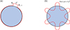Figure 3 Illustration of the condensation functions on the water disk: (a) gate function; (b) complex exponential function.

Using gate functions as condensation functions is equivalent to dividing the coupling/decoupling boundary Ω into a number of segments, as shown in Figure 3a. The gate functions are then defined on Ω according to their length L_ζ

$${\phi }^{\zeta }\left(\theta \right)=\{\begin{array}{l}\frac{1}{\sqrt{L_{\zeta }}}\hspace{0.33em} \mathrm{if}\hspace{0.33em} \theta \in \left[{\theta }_{\zeta -1},{\theta }_{\zeta }\right]\\ 0 \mathrm{elsewhere}\end{array},\zeta \in 1,N,$$(15)

where θ_ζ−1 and θ_ζ are the boundaries of the segment ζ. In practice, when using gate functions, the condensed transfer function between two segments of the subsystems is computed by exciting a single segment and measuring the response on the given receiving segment (while keeping all others rigid).

As it has already been observed in previous studies [11, 12], the number N of condensation functions taken into account for the calculation plays a key role in the convergence of the sub-structuring approach. The number of condensation functions follows a wavelength-based criterion at the highest considered frequency, accounting for the acoustic wavelength in the fluid and the flexural wavelength of the shell. In the considered frequency range, the flexural wavelength of the shell remains lower than the acoustic wavelength in the fluid, so the criterion will be based on the flexural wavelength of the shell. For the gate functions, it yields

$$L_{\zeta }\le \frac{{\lambda }_f}{2},$$(16)

where λ_f is the flexural wavelength of the shell.

Additionally, an alternative choice of condensation functions could be that of the complex exponential functions. As an example, it is illustrated on the water disk (i.e., subsystem 2) in Figure 3b. The complex exponential functions are defined on Ω as the set of N = 2K+1 condensation functions by the following

$${\phi }^{\zeta }\left(\theta \right)=\frac{1}{\sqrt{2\pi R}}{\mathrm{e}}^{\mathrm{j}\zeta \theta }, \zeta \in -K,K.$$(17)

When the condensation functions are complex exponentials, the boundary Ω is excited by a sinusoidal function for which the number of lobes corresponds to the index of the condensation function ζ in equation (17). Those functions are continuous on Ω, in contrast to the gate functions. For the complex exponential functions, the maximum index K is defined as

$$K\ge \frac{L_s}{{\lambda }_f}-\frac{1}{2},$$(18)

where L_s is the circumference of the shell.

2.3.2 Synthesis of the numerical procedure

Once the condensation functions have been defined, the CTFs can be calculated for each subsystem. In the present case, they are computed as follows:

• for Z₁₊₂ and ${\mathbf{P}}_{\mathbf{1}+\mathbf{2}}^{{\mathbf{M}}_{\mathbf{1}}}$, an analytical formulation is implemented with the image source method to account for the infinite reflections of acoustic waves off the waveguide boundaries [18].

• for Z₂, an analytical formulation is implemented based on a decomposition of the acoustic pressure on the circumferential orders of the subsystem.

• for Y₃ and ${\tilde{\mathbf{U}}}_{\mathbf{3}}$, an analytical formulation is implemented based on the resolution of Flügge’s equations of motion of the shell.

Details for these calculations are given in Appendix. Once these quantities have been calculated, the CTF-rCTF can be carried out:

• Z₁ is obtained from Z₂ and Z₁₊₂ from equation (10);

• ${\mathbf{Z}}_{\mathbf{1}}^{{\mathbf{M}}_{\mathbf{1}}}$ is deduced from ${\mathbf{P}}_{\mathbf{1}+\mathbf{2}}^{{\mathbf{M}}_{\mathbf{1}}}$ and the previous quantities using equation (14);

• U₁₊₃ is then evaluated using Y₃ and ${\tilde{\mathbf{U}}}_{\mathbf{3}}$ from equation (7);

• Finally, the radiated pressure in the fluid domain of an underwater waveguide is estimated using equation (8), ${\mathbf{Z}}_{\mathbf{1}}^{{\mathbf{M}}_{\mathbf{1}}}$ and the previous quantities.

3 Results and discussion

The numerical process described in the previous section is now applied to predict the vibration and sound radiated from the shell excited by a radial harmonic force at a point θ = 0 (i.e., a vertical load at the bottom of the shell) of an infinitely-long cylindrical shell under a harmonic line force and immersed in a perfect underwater waveguide. All the parameters of the calculation (i.e., dimensions of the shell, material properties of the shell and of the surrounding fluid) are given in Table 1. The calculation is performed between 5 Hz and 3000 Hz with 5 Hz increments, as to maintain a consistent comparison with the results obtained in Ref. [18].

In the following study, the two vibroacoustic indicators of interest include:

• the pressure radiated by the shell at a point located at 1 m to the right from the surface of the shell, that is a point of coordinate (0,1+R) (see Fig. 1). This quantity is obtained using equation (8) (as described in Sect. 2.3.2), and,

• the mean quadratic velocity of the shell which is expressed by

$$\langle u^2\rangle =\frac{1}{2\pi R}\underset{0}{\overset{2\pi }{\int }}\mathrm{}\left|u\right(\theta ){|}^{2}R\mathrm{d}\theta =\frac{1}{2\pi R}\sum _{\zeta }\mathrm{}|U_{1+3}^{\zeta }{|}^2,$$(19)

where U₁₊₃ is obtained from equation (7).

3.1 Using gate functions as the condensation functions

The gate functions are chosen as the condensation functions to be used in the CTF-rCTF approach. According to the criteria related to the number of condensation functions (see Eq. 16), it is necessary to divide Ω into 110 gates (N = 110). The results are then presented in Figures 4 and 5, and compared against the analytical solution from Ref. [18]. For the structural response, which is presented as a mean quadratic velocity, the result is shown in Figure 4. The result obtained by the CTF-rCTF approach seem to provide the same number of resonances that is consistent with the analytical result. However, there are issues with amplitude and slight frequency shifts throughout the frequency range. For the acoustic response, which is presented as a radiated sound pressure level received at a point in the fluid domain, the result is shown in Figure 5. It is shown that the general trend of the spectrum matches with the analytical solution. However, throughout the frequency range, there are discrepancies in the form of the persistence of singularities in the fluid domain. It can be explained from the application of gate functions, which have an inherent piece-wise description, that the convergence to the correct solution can be difficult. The bounds of each gate presents a discontinuity whereas the physics that is described (i.e., wave propagation) is continuous by nature. This does not lead to significant discrepancies in many applications in light fluid (see Refs. [8, 24]). In the present case of a heavy fluid loaded structure, these discontinuities in the reconstructed velocity field at the junction between the shell and fluid can lead to the frequency shift observed here. As it has been previously stated, the convergence of the calculation is directly linked with the number of condensation functions. The criterion proposed in equation (16) led us to divide Ω into 110 gates. To ensure that this criterion is sufficient and that the poor results observed in Figures 4 and 5 are indeed linked to the piecewise nature of the condensation function rather than the insufficient number of gates, a calculation was performed up to 1000 Hz using 199 and 331 gates (corresponding respectively to a λ/6 and λ/10 criterion at 1000 Hz). The results from those two calculation are not shown here as they did not significantly differ from what was obtained with the λ/2 criterion, which means that the lack of convergence is not linked to the number of condensation functions here. This result could have been expected as the discrepancies appear also in the low-frequency range, while a poor convergence due to an insufficient number of condensation functions would have converged in the low frequencies, up until a cutoff frequency for which the criterion would not have been sufficient anymore. Therefore, it is demonstrated in the following discussions, the possibility to improve the result by applying an improvement to the CTF-rCTF procedure.

Figure 4 Mean square velocity of the shell.

Figure 5 Pressure radiated from the shell.

3.2 Improvement of the process by partitioning outside the near field of the shell

It is shown in previous studies related to sub-structuring approaches (see, for example, Ref. [25] for the PTF method) that partitioning the subsystems at the fluid-structure interface leads to poor convergence of the method for the case of heavy fluid. Indeed, for frequencies well below the critical frequency (which is the case here), the pressure in the near field of the structure varies mainly according to the flexural wavelength of the structure. To circumvent this issue, Maxit et al. [26] proposed to shift the coupling boundary inside the fluid domain at a sufficiently large distance from the structure so it can be considered that the partitioning is no longer located in its near field. Following this suggestion, a new subtractive modeling problem is proposed, illustrated in Figure 6. Instead of considering the uncoupled cylindrical shell for the recoupling procedure (subsystem 3), the recoupled subsystem is a cylindrical shell coupled to a thin fluid layer for which the thickness is determined according to the procedure described in [26] (h_f = 0.3 m). Subsequently, the removed subsystem of the decoupling procedure (subsystem 2) will be a water disk of the same size of the volume occupied by the shell surrounded by the fluid layer.

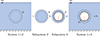Figure 6 Subtractive modeling when partitioning outside of the near field of the shell.

As a result of this change in the subsystems, a new formulation must be derived. This new formulation differs from the one in Section 2.2 in the recoupling procedure, as we are dealing now with acoustic boundaries only. As such, condensed impedances instead of condensed admittances must be computed for subsystem 3, which is the cylindrical shell surrounded by a fluid layer. Similarly, condensed pressures must be computed instead of condensed admittances. The superposition principle of equation (5) becomes

$$\{\begin{array}{l}{\mathbf{P}}_{\mathbf{1}}={\mathbf{Z}}_{\mathbf{1}}{\mathbf{U}}_{\mathbf{1}},\\ {\mathbf{P}}_{\mathbf{3}}={\tilde{\mathbf{P}}}_{\mathbf{3}}+{\mathbf{Z}}_{\mathbf{3}}{\mathbf{U}}_{\mathbf{3}},\end{array}$$(20)

with Z₃ being the condensed impedance matrix of subsystem 3 and ${\tilde{\mathbf{P}}}_{\mathbf{3}}$ the vector of the condensed pressures at the boundary Ω induced by the external mechanical force applied on the shell. The continuity conditions of equation (6) remain unchanged, allowing to express the coupling condensed velocities

$${\mathbf{U}}_{\mathbf{1}+\mathbf{3}}=-{\left({\mathbf{Z}}_{\mathbf{1}}+{\mathbf{Z}}_{\mathbf{3}}\right)}^{-1}{\tilde{\mathbf{P}}}_{\mathbf{3}}.$$(21)

where Z₁ is given by equation (10). To compute the radiated pressure from the knowledge of the coupling velocities, it is necessary to make the distinction between a point located outside of Ω (initially belonging to subsystem 1) and a point located inside of Ω (initially belonging to the fluid layer in subsystem 3). For the first case scenario, the pressure at point M₁ located outside of Ω can be expressed as

$$p_{1+2}\left(M_1\right)=-{\left({\mathbf{Z}}_{\mathbf{1}}^{{\mathbf{M}}_{\mathbf{1}}}\right)}^T{\left({\mathbf{Z}}_{\mathbf{1}}+{\mathbf{Z}}_{\mathbf{3}}\right)}^{-1}{\tilde{\mathbf{P}}}_{\mathbf{3}},$$(22)

where ${\mathbf{Z}}_{\mathbf{1}}^{{\mathbf{M}}_{\mathbf{1}}}$ is given by equation (14). As for the pressure at M₃ located inside of Ω

$$p_{1+2}\left(M_3\right)={\tilde{p}}_3\left(M_3\right)+{\left({\mathbf{P}}_{\mathbf{3}}^{{\mathbf{M}}_{\mathbf{3}}}\right)}^T{\left({\mathbf{Z}}_{\mathbf{1}}+{\mathbf{Z}}_{\mathbf{3}}\right)}^{-1}{\tilde{\mathbf{P}}}_{\mathbf{3}},$$(23)

Where

• ${\tilde{p}}_3\left(M_3\right)$ is the pressure radiated at point M₃ of the uncoupled subsystem 3 induced by the external mechanical force applied on the shell.

• ${\mathbf{P}}_{\mathbf{3}}^{{\mathbf{M}}_{\mathbf{3}}}$ is the vector of the condensed pressures at the surface Ω of the uncoupled subsystem 3, induced by a monopole source of unit volume velocity located at point M₃.

One of the consequences of this alternative formulation is that, as we are dealing now with acoustic boundaries only, the criterion established in equation (16) now refers to the acoustic wavelength in the fluid, which is greater than the flexural wavelength of the shell. This means that, in theory, less gate functions are necessary to correctly converge at the highest considered frequency. Following this criterion, the decoupling boundary Ω must be divided into 33 gates to ensure convergence at 3000 Hz. However, after a convergence check, it appeared that the calculation reached convergence using 133 gates instead of 33, which is related to a criterion close to λ/8. The results presented in this paragraph are then obtained using 133 gates.

In the following, the point at which the calculations are performed is located outside of Ω, meaning that only equation (22) is of interest in this paragraph. As such, the procedure for the calculation of Z₃ and ${\tilde{\mathbf{P}}}_{\mathbf{3}}$ using an analytical formulation is detailed in Appendix. In this section, the vibration response of the shell is not investigated as it would require supplementary calculations from the fact that Ω is no longer located at the exterior radius of the shell. The new result for the radiated sound pressure level is then shown in Figure 7. It is observed that the comparison against the analytical result is significantly improved. Especially at the low frequency range (approximately up to 700 Hz), the agreement is excellent. However, beyond this frequency range, some discrepancies are evident even if the global tendencies are well respected. These discrepancies can be attributed to the common anti-resonances between the waveguide (system 1+2) and the water disk (subsystem 2), which arise as an effect from the decoupling process. This has been previously observed in Ref. [13].

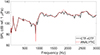Figure 7 Pressure radiated by the shell when partitioning outside of the near-field of the shell.

3.3 Using complex exponential functions as the condensation functions

The calculations have been performed considering the initial partitioning (i.e., at the surface of the shell) and the complex exponential functions as condensation functions. Using the criterion defined by equation (18) for the complex exponential functions, a maximum index K = 55 (N = 111) for the complex exponential functions. The mean quadratic velocity is shown in Figure 8, and the radiated sound pressure level in Figure 9. From these results, it is observed that: (a), an excellent agreement between the CTF-rCTF and the analytical results; (b) an improvement of the calculation convergence compared to the results considering the gate functions (as shown in Figs. 4 and 5). The only notable discrepancy is in the radiated sound pressure level at some particular frequencies. As described previously, it is owed to anti-resonances that appear in the decoupling process. However, in this case, the effect is much less impactful on the result, and the acoustic response achieves a very good comparison. Therefore, the sub-structuring technique of CTF-rCTF is validated against the analytical result. In general, any orthonormal function can be applied to condense the transfer functions. In previous studies, the complex exponential function has been applied as CFs to contrast the gate functions. It can be inferred from the analytical approaches in solving the shell equations that the circumferential Fourier decomposition involves complex exponential functions. Therefore, it is not surprising that the complex exponential functions perform better in CFs than the gate functions as shown from the better agreement of results. It can better model the natural circumferential modal shapes of the cylindrical shell.

Figure 8 Mean square velocity of the shell using complex exponentials as condensation functions.

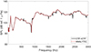Figure 9 Pressure radiated by the shell using complex exponentials as condensation functions.

4 Conclusions

A two-dimensional vibroacoustic model of a forced cylindrical shell immersed in an underwater waveguide has been developed using the CTF-rCTF coupling/decoupling technique. The model of target system is obtained from a perfect underwater waveguide that is decoupled with a water disk. The excited shell is then coupled in-place of the water disk. The numerical process to address this fluid-structure problem as well as the analytical expressions of the condensed transfer functions for the different subsystems have been proposed in this paper. In order to study the convergence of the proposed process, the results were compared and verified against corresponding ones from an analytical calculation.

It was recognized that partitioning the system at the fluid-structure interface and using gate functions as the choice of CFs can lead to some inaccuracies in the prediction. For this case of a vibrating structure immersed in heavy fluid, the results have been improved by considering two different options: (a) including a layer of fluid domain that extends beyond the near field surrounding the shell; (b) by using the complex exponential functions as the CFs. For future works, the use of complex exponential functions as CFs with partitioning at the structure surface is recommended. The results are accurate whereas the CTFs of the structure can be easily estimated with a finite element model by using modal expansion. In the framework of the CTF-rCTF developments, the novelty of these investigations involves complicating the fluid domain by adding acoustic boundaries and heavy fluid loading, rather than complicating the structural component of the system, which has been done in the past [11, 12]. It is anticipated that this preliminary effort will inspire future analysis of complex vibroacoustic systems that involve complex structural geometries and fluid domains with acoustic boundaries. As an example of future work, the investigation could be tailored to a system of a submarine in shallow waters. The objective to investigate the 3-D counterpart of the preliminary study could involve the finite-length cylindrical shell immersed in a shallow water environment, such as the Pekeris waveguide and range-dependent waveguides, such that reflections on the seabed are dependent on the incident angle and the profile changes of the seabed. This provides a more realistic influence of acoustic propagation in shallow water. The cylindrical shell could be further complicated by involving conical end-caps, stiffener structures and bulkheads that converge the numerical simulation to a more realistic construction.

Conflicts of interest

The authors declare that they have no known competing financial interests of personal relationships that could have appeared to influence the work reported in this paper.

Data availability statement

Data are available on request from the authors.

Appendix

Condensed impedances of the perfect acoustic waveguide

A.1 Condensed impedances of the perfect acoustic waveguide

The condensed impedances of the perfect waveguide constituting system 1+2 are defined by equation (2). They are calculated by applying on Ω a velocity jump corresponding to a condensation function. To emulate this velocity jump, an integral formulation is considered where the pressure field can be expressed from the single layer potential due to a layer of monopole sources [13]

$$p\left(M\right)={\iint }_{\mathrm{\Omega }}\mathrm{}\nu \left(P\right)G(M,P)\mathrm{\Omega }\left(P\right), M\in \mathrm{\Omega }, P\in \mathrm{\Omega },$$(A1)

with ν(P) being the single layer potential, and G(M,P) the Green function of the system, corresponding to the response at point P when a monopole is located at point M. The Green function of the system can be calculated using the image-source method [18] to account for the infinite reflections of acoustic waves off the waveguide boundaries. The principle of this approach is that an infinite number of identical monopole sources exist due to the reflections off the free surface, rigid floor and both, as illustrated in Figure A1. For a perfect acoustic waveguide, the free surface has a reflection coefficient of −1, and the rigid floor has a reflection coefficient of +1. With this in mind, it is convenient to label the free surface as (−) and the rigid floor as (+). In this way, the acoustic waves travelling from the images to the observer point will “pass” through the acoustic boundaries and collect the sign of the acoustic boundaries it has passed through. For example, the upper image 2 will collect (−)(+).

Figure A1 Schematic diagram of the image-source method.

Following this approach, the Green function for the monopole source between points M(x₁,y₁) and P(x₂,y₂) can be written

$$G_{\mathrm{WG}}(x_1,y_1|x_2,y_2)=G_{\mathrm{FF}}(x_1,y_1|x_2,y_2)+\sum _{i=1}^{\infty }\mathrm{}{R}^i{G}^i(x_1,y_1|x_2,y_2),$$(A2)

where G_FF is the Green’s function for the original monopole source, which is equivalent to the free-field Green function, Rⁱ are corresponding coefficients based on reflection for the Green functions of the image monopole sources Gⁱ. The following distances and coefficients it collects between the image sources and the observer point are determined to be

for upper images

$$\{\begin{array}{ll}\sqrt{(x_2-x_1{)}^2+(y_2-2H_{\mathrm{fs}}+y_1{)}^2} & \mathrm{and} (-),\\ \sqrt{(x_2-x_1{)}^2+(y_2-2H_{\mathrm{fs}}-y_1{)}^2} & \mathrm{and} (-)(+),\\ \sqrt{(x_2-x_1{)}^2+(y_2-2H-2H_{\mathrm{fs}}+y_1{)}^2} & \mathrm{and} (-)(+)(-),\\ \sqrt{(x_2-x_1{)}^2+(y_2-4H-y_1{)}^2} & \mathrm{and} (-)(+)(-)(+),\\ \dots & \end{array}$$(A3)

and

for lower images

$$\{\begin{array}{ll}\sqrt{(x_2-x_1{)}^2+(y_2+2H_{\mathrm{sb}}+y_1{)}^2} & \mathrm{and} (-),\\ \sqrt{(x_2-x_1{)}^2+(y_2+2H_{\mathrm{fs}}-y_1{)}^2} & \mathrm{and} (-)(+),\\ \sqrt{(x_2-x_1{)}^2+(y_2+2H+2H_{\mathrm{sb}}+y_1{)}^2} & \mathrm{and} (-)(+)(-),\\ \sqrt{(x_2-x_1{)}^2+(y_2+4H-y_1{)}^2} & \mathrm{and} (-)(+)(-)(+),\\ \dots .& \end{array}$$(A4)

It is recognized that there are four unique cases for the images: reflection off the free surface (−), reflection off the rigid floor (+), reflection off the free surface and then the rigid floor (−)(+), and reflections off the rigid floor and then the free surface (+)(−). Subsequent reflections are encompassed by one of these four unique cases. Thus, the Green function can be expressed as

$$\begin{array}{c}{G}_{\mathrm{WG}}(x_1,y_1|x_2,y_2)=G_{\mathrm{FF}}(x_1,y_1|x_2,y_2)+\sum _{i=1}^{\infty }\mathrm{}\left[\right(-1\left)\right(+1){]}^{i-1}\\ \cdot \left((-1)G_{(-)}^i+(+1)G_{(+)}^i+(-1)(+1)G_{(-)(+)}^i+(+1)(-1)G_{(+)(-)}^i\right).\end{array}$$(A5)

These Green functions take the form of the zero-th order Hankel function of the second kind (assuming e^jωt)

$$G_{\mathrm{FF}}=\frac{-j}{4}{H}_0^{\left(2\right)}\left(\mathrm{kr}\right), G_M^i=\frac{-j}{4}{H}_0^{\left(2\right)}\left(k{r}_M^i\right)$$(A6)

The distances for the image sources are given as

$$r_M^i=\{\begin{array}{ll}\sqrt{(x_2-x_1{)}^2+(y_2-2H(i-1)-2H_{\mathrm{fs}}+y_1{)}^2} & \mathrm{if} M=(-),\\ \sqrt{(x_2-x_1{)}^2+(y_2-2H(i-1)+2H_{\mathrm{sb}}+y_1{)}^2} & \mathrm{if} M=(+),\\ \sqrt{(x_2-x_1{)}^2+(y_2-2\mathrm{Hi}-y_1{)}^2} & \mathrm{if} M=(-)(+),\\ \sqrt{(x_2-x_1{)}^2+(y_2+2\mathrm{Hi}-y_1{)}^2} & \mathrm{if} M=(+)(-),\\ \dots .& \end{array}$$(A7)

It is important to mention that the sum in equation (A5) is infinite. In practice, it is truncated to a finite value N, which has been set to N = 300 for this study in order to obtain a correct convergence of the calculation while keeping the computing time relatively low. Now that the Green function of the system has been defined, the pressure in the waveguide due to a velocity jump corresponding to a condensation function φ^ξ is given by

$$p_{1+2}\left({\theta }_M\right)=\mathrm{j}\omega {\rho }_0{\int }_0^{2\pi }\mathrm{}{\phi }^{\xi }\left({\theta }_P\right)G({\theta }_M,{\theta }_P){\theta }_P,$$(A8)

with the single layer potential being ν(P) = jωρ₀φ^ξ(θ_P), and ρ₀ the fluid density. Then, the condensed impedance between φ^ξ and φ^ζ is

$$Z_{1+2}^{\zeta \xi }=\mathrm{j}\omega {\rho }_0{R}^2{\int }_0^{2\pi }\mathrm{}{\int }_0^{2\pi }\mathrm{}{\phi }^{\xi }\left({\theta }_P\right)G({\theta }_M,{\theta }_P){\phi }^{\zeta \mathrm{*}}\left({\theta }_M\right){\theta }_P{\theta }_M.$$(A9)

In practice, the integrals in equation (A9) are discretized into a finite sum corresponding to the number R of monopole sources constituting the single layer potential

$$Z_{1+2}^{\zeta \xi }=\mathrm{j}\omega {\rho }_0{R}^2\sum _{r=1}^R\mathrm{}\sum _{q=1}^R\mathrm{}{\phi }^{\xi }\left({\theta }_P^q\right)G({\theta }_M^r,{\theta }_P^q){\phi }^{\zeta \mathrm{*}}\left({\theta }_M^r\right)\delta {\theta }^2.$$(A10)

When the condensation functions are gate functions, according to their definition in equation (15), and assuming both gates are discretized into the same number S of points constituting the monopoles and have the same length

$$Z_{1+2}^{\zeta \xi }=\frac{\mathrm{j}\omega {\rho }_{0}R}{{\theta }_{\max }-{\theta }_{\min }}\sum _{s=1}^S\mathrm{}\sum _{q=1}^S\mathrm{}G({\theta }_M^s,{\theta }_P^q)\delta {\theta }^2,$$(A11)

where θ_max−θ_min corresponds to the angular difference between two boundaries of a gate. The total number R of monopoles on Ω and the number S of monopoles in a gate are linked via the following relation R = N × S, where N is the number of gates.

When the condensation functions are complex exponentials, according to their definition in equation (17)

$$Z_{1+2}^{\zeta \xi }=\frac{\mathrm{j}\omega {\rho }_{0}R}{2\pi }\sum _{r=1}^R\mathrm{}\sum _{q=1}^R\mathrm{}G({\theta }_M^r,{\theta }_P^q){\mathrm{e}}^{\mathrm{j}\theta (\xi -\zeta )}\delta {\theta }^2.$$(A12)

Similarly, the condensed pressure term appearing in equation (14), corresponding to the pressure on Ω, projected on the condensation function φ^ξ, when the excitation is a monopole of unit volume velocity located at point M₁, can be expressed from the discretization of equation (A8)

$$P_{1+2}^{M_1,\xi }=\mathrm{j}\omega {\rho }_{0}R\sum _{q=1}^R\mathrm{}{\phi }^{\xi }\left({\theta }_P^q\right)G\left({\theta }_{M_1},{\theta }_P^q\right)\delta \theta .$$(A13)

This expression is made possible by the reciprocity principle [22, 23], stating that the pressure on Ω due to a monopole source located at M₁ is equivalent to the pressure at M₁ due to a layer of monopole source on Ω. Then, the expression of equation (A13) can be applied for the gate functions as

$$P_{1+2}^{M_1,\xi }=\frac{\mathrm{j}\omega {\rho }_0}{\sqrt{{\theta }_{\max }-{\theta }_{\min }}}\sum _{q=1}^S\mathrm{}G\left({\theta }_{M_1},{\theta }_P^q\right)\delta \theta ,$$(A14)

and for complex exponentials as

$$P_{1+2}^{M_1,\xi }=\frac{\mathrm{j}\omega {\rho }_0}{\sqrt{2\pi }}\sum _{q=1}^S\mathrm{}G\left({\theta }_{M_1},{\theta }_P^q\right){\mathrm{e}}^{\mathrm{j}\theta \xi }\delta \theta ,$$(A15)

A.2 Condensed impedances of the water disk

The condensed impedances of the water disk are calculated from their definition in equation (3). For this subsystem, an analytical formulation is implemented based on a decomposition of the acoustic pressure on the circumferential orders of the subsystem. In practice, the calculation is performed in the wavenumber domain by means of a Fourier series decomposition along θ defined as

$$\tilde{f}\left(n\right)=\frac{1}{2\pi }{\int }_0^{2\pi }\mathrm{}f\left(\theta \right){\mathrm{e}}^{-\mathrm{j}n\theta }\theta \hspace{0.33em} \mathrm{and} \hspace{0.33em}f\left(\theta \right)=\sum _{n=-\infty }^{\infty }\mathrm{}\tilde{f}\left(n\right){\mathrm{e}}^{\mathrm{j}n\theta }.$$(A16)

Using this formalism, the pressure in the water disk can be expressed as

$$\tilde{p}(r,n)=A_n{J}_n\left(k_{0}r\right)+B_n{Y}_n\left(k_{0}n\right),$$(A17)

where J_n and Y_n are the Bessel functions of the first and second kind, respectively. Then, the unknowns A_n and B_n can be inferred from the boundary conditions of the system. When r tends to 0, Y_n tends to infinity; as the pressure is finite in r = 0, B_n must necessarily be 0. When r = R, the Euler condition must be satisfied (assuming e^jωt)

$$\frac{\partial p}{\partial r}(r=R,\theta )=-\mathrm{j}\omega {\rho }_0{\phi }^{\xi }\left(\theta \right),$$(A18)

where ρ₀ is the density of the fluid, and φ^ξ is the condensation function associated with the excitation. From those boundary conditions, the circumferential pressure at the surface of the disk p(R,θ) can be expressed as

$$p(R,\theta )=-\sum _{n=-\infty }^{\infty }\mathrm{}\frac{\mathrm{j}\omega {\rho }_0{J}_n\left(k_{0}R\right)}{k_0{J}_n^{\mathrm{\prime }}\left(K_{0}R\right)}{\tilde{\phi }}^{\xi }\left(n\right){\mathrm{e}}^{\mathrm{j}n\theta },$$(A19)

with $J_n^{\mathrm{\prime }}$ being the derivative of the Bessel function of the first kind with respect to its argument. Then, from equation (3), the condensed impedance between φ^ξ and φ^ζ is

$$Z_2^{\zeta \xi }=-2\pi R\sum _{n=-\infty }^{\infty }\mathrm{}\frac{\mathrm{j}\omega {\rho }_0{J}_n\left(k_{0}R\right)}{k_0{J}_{\mathrm{n\text{'}}}\left(K_{0}R\right)}{\tilde{\phi }}^{\xi }\left(n\right){\tilde{\phi }}^{\zeta \mathrm{*}}\left(n\right).$$(A20)

When the condensation functions are gate functions, equation (A20) must be applied with

$${\tilde{\phi }}^{\xi }\left(n\right)=\frac{1}{2\pi }\sqrt{\frac{{\theta }_{\max }^{\xi }-{\theta }_{\min }^{\xi }}{R}}{\mathrm{e}}^{-\mathrm{j}n\left(\frac{{\theta }_{\max }^{\xi }+{\theta }_{\min }^{\xi }}{2}\right)}\mathrm{sinc}\left(n\frac{{\theta }_{\max }^{\xi }-{\theta }_{\min }^{\xi }}{2}\right),$$(A21)

where ${\theta }_{\max }^{\xi }$ and ${\theta }_{\max }^{\xi }$ are the boundaries of the segment ζ, and sinc is the cardinal sinus function. Once again, the sum in equation (A20) must be truncated to a finite value. In this work, this value was chosen to be N = 200. As the calculation is analytical, the calculation time remains very low for this subsystem.

When the condensation functions are complex exponentials, by deduction from the definition of the Fourier series decomposition in equation (A16)

$${\tilde{\phi }}^{\xi }\left(n\right)=\{\begin{array}{ll}-\frac{1}{2\pi R} & \mathrm{if} n=\xi ,\\ 0 & \mathrm{otherwise}.\end{array}$$(A22)

Then, the condensed impedance between φ^ξ and φ^ζ is

$$Z_2^{\zeta \xi }=\{\begin{array}{ll}-\frac{\mathrm{j}\omega {\rho }_0{J}_{\xi }\left(k_{0}R\right)}{k_O{J}_{\xi \text{'}}\left(k_{0}R\right)} & \mathrm{if} \xi =\zeta ,\\ 0 & \mathrm{otherwise}.\end{array}$$(A23)

A.3 Condensed admittances of the uncoupled cylindrical shell

The condensed admittances of the uncoupled cylindrical shell are calculated from their definition in equation (4). For this subsystem, an analytical formulation is implemented based on the resolution of the Flügge’s equations of motion of the shell [18, 27]. Following this theory, the radial displacement of the uncoupled shell in response to a mechanical excitation corresponding to a condensation function can be described as

$$\frac{1}{\gamma }\left(-\frac{\frac{{\mathrm{d}}^2}{{\mathrm{d}\theta }^2}}{\frac{{\mathrm{d}}^2}{{\mathrm{d}\theta }^2}+R^2{\mathrm{\Phi }}^2}+K^2\frac{{\mathrm{d}}^4}{{\mathrm{d}\theta }^4}+2\frac{{\mathrm{d}}^2}{{\mathrm{d}\theta }^2}+1+K^2-R^2{\mathrm{\Phi }}^2\right)w\left(\theta \right)={\phi }^{\xi },$$(A24)

where w is the radial displacement of the shell, $\gamma =R^2(1-{\nu }_s^2)/E_s{h}_s$, $\mathrm{\Phi }=\omega \sqrt{{\rho }_s{R}^2(1-{\nu }_s^2)/E_s}$ is a frequency parameter non-dimensionalized by the ring frequency of the shell, and $K = h_s^2/\left(12R^2\right)$. Similarly to the calculation of the condensed impedances of the water disk in Appendix A.2, the problem is solved in the wavenumber domain by the means of a Fourier series decomposition along θ, defined in equation (A16). Equation (A24) can be re-written in the Fourier domain as

$$\frac{1}{\gamma }\left(-\frac{n^2}{n^2-R^2{\mathrm{\Phi }}^2}+1+K(n^4-2n^2+1)-R^2{\mathrm{\Phi }}^2\right)\tilde{W}\left(n\right)={\tilde{\phi }}^{\xi }\left(n\right),$$(A25)

where $\tilde{W}\left(n\right)$ and ${\tilde{\phi }}^{\xi }\left(n\right)$ are the Fourier series coefficients of the shell radial displacement and condensation function excitation, respectively. Then, the Fourier displacement coefficients can be solved by inverting equation (A25)

$$\begin{array}{ll}\tilde{W}\left(n\right)& =\gamma {\left(-\frac{n^2}{n^2-R^2{\mathrm{\Phi }}^2}+1+K(n^4-2n^2+1)-R^2{\mathrm{\Phi }}^2\right)}^{-1}{\tilde{\phi }}_{\xi }\left(n\right)\\ & =\gamma T^{-1}{\tilde{\phi }}^{\xi }\left(n\right).\end{array}$$(A26)

The radial displacement is then expressed as

$$w\left(\theta \right)=\gamma \sum _{n=-\infty }^{\infty }\mathrm{}{T}^{-1}{\tilde{\phi }}^{\xi }\left(n\right){\mathrm{e}}^{\mathrm{j}n\theta }.$$(A27)

In practice, to compute the condensed admittances and velocities of the uncoupled shell

The condensed admittance between φ^ξ and φ^ζ is then

$$Y_3^{\zeta \xi }=2\pi R\gamma \sum _{n=-\infty }^{\infty }\mathrm{}{T}^{-1}{\tilde{\phi }}^{\xi }\left(n\right){\tilde{\phi }}^{\zeta \mathrm{*}}\left(n\right).$$(A28)

When the condensation functions are gate functions, equation (A28) must be applied, with ${\tilde{\phi }}^{\psi }$ (ψ = ξ or ζ) being determined by equation (A21). While, for condensation functions being complex exponentials, equation (A22) allows expressing the condensed admittance as

$$Y_3^{\zeta \xi }=\{\begin{array}{ll}\gamma T^{-1} & \mathrm{if} \xi =\zeta ,\\ 0 & \mathrm{otherwise}.\end{array}$$(A29)

Alternatively, to calculate the condensed velocity term of the uncoupled shell appearing in equation (8), the circumferential radial velocity can be expressed from equation (A26), with the mechanical excitation term replacing the condensation function excitation

$$\tilde{W}\left(n\right)=\gamma T^{-1}{F}_n,$$(A30)

with $F_n=\frac{{\mathrm{e}}^{-\mathrm{j}n{\theta }_0}}{2\pi R}$, θ₀ being the angle of application of the force. The radial displacement can then be expressed as

$$w\left(\theta \right)=\frac{\gamma }{2\pi R}\sum _{n=-\infty }^{\infty }\mathrm{}{T}^{-1}{\mathrm{e}}^{\mathrm{j}n(\theta -{\theta }_0)}.$$(A31)

The condensed velocity can then be obtained by projecting the expression of equation (A31) on the condensation function φ^ξ

$$U_3^{\xi }=\gamma \sum _{n=-\infty }^{\infty }\mathrm{}{T}^{-1}{\tilde{\phi }}^{\xi }\left(n\right){\mathrm{e}}^{-\mathrm{j}n{\theta }_0}$$(A32)

When the condensation functions are gate functions, equation (A32) must be applied, with ${\tilde{\phi }}^{\xi }$ being determined by equation (A21). While, for condensation functions being complex exponentials, equation (A22) allows expressing the condensed velocity as

$$U_3^{\xi }=\frac{\gamma }{\sqrt{2\pi R}}{T}^{-1}{\mathrm{e}}^{-\mathrm{j}\xi {\theta }_0}$$(A33)

A.4 Condensed impedances of the cylindrical shell surrounded by a layer of water

In Section 3.2, the partitioning is performed outside of the near field of the shell, and the recoupled subsystem is now the cylindrical shell surrounded by a layer of water (see Fig. 6). As the boundary Ω is acoustic, the condensed transfer functions of this subsystem will be condensed impedances and are defined according to equation (3). Once again, the calculation is performed in the wavenumber domain as in Appendix A.2. The circumferential pressure in the water layer is reminded

$$\tilde{p}(r,n)=A_n{J}_n\left(k_{0}r\right)+B_n{Y}_n\left(k_{0}n\right).$$(A34)

Now, to solve the considered problem, the calculation must be done in two steps. The first one consists of expressing the circumferential fluid loading impedance ${\tilde{Z}}_f$. The second step consists of expressing the blocked pressure (i.e., the pressure in the fluid layer arising from the prescribed velocity, as though the shell was rigid) at the surface of the shell. This blocked pressure will then serve as a mechanical excitation term to express the total pressure on Ω.

A.4.1 Calculation of the circumferential fluid loading impedance

To calculate the circumferential fluid loading impedance, the solutions of equation (A34) are re-written

$${\tilde{p}}_{\mathrm{imp}}(r,n)=A_n^{\mathrm{imp}}{J}_n\left(k_{0}r\right)+B_n^{\mathrm{imp}}{Y}_n\left(k_{0}r\right).$$(A35)

This problem can be solved by considering the boundary conditions, which are the rigid boundary of the external fluid layer and the kinematic condition at the shell’s surface assuming unit displacement of the shell. They yield

$$\{\begin{array}{l}\frac{\partial \tilde{p}}{\partial r}(r=R,n)={\rho }_0{\omega }^2,\\ \frac{\partial \tilde{p}}{\partial r}(r=R_{\mathrm{ext}},n)=0.\end{array}$$(A36)

The resolution of the system of equation (A36) allows expressing the circumferential pressure in the fluid layer as

$$\begin{array}{ll}\tilde{p}(r,n)& =\frac{{\rho }_0{\omega }^2}{k_0}\frac{J_{\mathrm{n\text{'}}}\left(k_0{R}_{\mathrm{ext}}\right)Y_n\left(k_{0}r\right)-Y_{\mathrm{n\text{'}}}\left(k_0{R}_{\mathrm{ext}}\right)J_n\left(k_{0}r\right)}{J_{\mathrm{n\text{'}}}\left(k_0{R}_{\mathrm{ext}}\right)Y_{\mathrm{n\text{'}}}\left(k_{0}R\right)-J_{\mathrm{n\text{'}}}\left(k_{0}R\right)Y_{\mathrm{n\text{'}}}\left(k_0{R}_{\mathrm{ext}}\right)}\\ & =\frac{{\rho }_0{\omega }^2}{k_0}{\mathrm{\Theta }}_n^{\mathrm{imp}}(r,n).\end{array}$$(A37)

The circumferential fluid loading impedance can then be expressed as

$${\tilde{Z}}_f=\tilde{p}(R,n)=\frac{{\rho }_0{\omega }^2}{k_0}{\mathrm{\Theta }}_n^{\mathrm{imp}}(r=R,n).$$(A38)

A.4.2 Calculation of the blocked circumferential pressure at the surface of the shell

To calculate the circumferential fluid loading impedance, the solutions of equation (A34) are re-written

$${\tilde{p}}_{\mathrm{blo}}(r,n)=A_n^{\mathrm{blo}}{J}_n\left(k_{0}r\right)+B_n^{\mathrm{blo}}{Y}_n\left(k_{0}r\right).$$(A39)

Once again, the following boundary conditions are used to solve this problem. At the exterior surface of the fluid layer, a prescribed velocity ${\tilde{\phi }}_{\zeta }\left(n\right)$ is imposed, while the surface of the shell is considered rigid. The Euler relation then yields

$$\{\begin{array}{l}\frac{\partial \tilde{p}}{\partial r}(R,n)=0,\\ \frac{\partial \tilde{p}}{\partial r}(R_{\mathrm{ext}},n)=-\mathrm{j}\omega {\rho }_0{\tilde{\phi }}^{\zeta }\left(n\right).\end{array}$$(A40)

The resolution of this system of equations allows expressing the blocked pressure in the fluid layer as

$$\begin{array}{ll}{\tilde{p}}_{\mathrm{blo}}(r,n)& =-\frac{\mathrm{j}{\rho }_0\omega }{k_0}\frac{J_{\mathrm{n\text{'}}}\left(k_{0}R\right)Y_n\left(k_{0}r\right)-Y_{\mathrm{n\text{'}}}\left(k_{0}R\right)J_n\left(k_{0}r\right)}{J_{\mathrm{n\text{'}}}\left(k_0{R}_{\mathrm{ext}}\right)Y_{\mathrm{n\text{'}}}\left(k_{0}R\right)-J_{\mathrm{n\text{'}}}\left(k_{0}R\right)Y_{\mathrm{n\text{'}}}\left(k_0{R}_{\mathrm{ext}}\right)}{\tilde{\phi }}^{\zeta }\left(n\right)\\ & =-\frac{\mathrm{j}{\rho }_0\omega }{k_0}{\mathrm{\Theta }}_n^{\mathrm{blo}}(r,n){\tilde{\phi }}^{\zeta }\left(n\right).\end{array}$$(A41)

The blocked pressure at the surface of the shell is then

$${\tilde{p}}_{\mathrm{blo}}(R,n)=-\frac{\mathrm{j}{\rho }_0\omega }{k_0}{\mathrm{\Theta }}_n^{\mathrm{blo}}(r=R,n){\tilde{\phi }}^{\zeta }\left(n\right).$$(A42)

A.4.3 Resolution of the problem

The problem can now be solved classically by using the Flügge’s operator to express the circumferential radial displacement of the shell as

$$\tilde{W}\left(n\right)=\frac{\gamma {\tilde{p}}_{\mathrm{blo}}(R,n)\left({\tilde{Z}}_{\mathrm{UU}}{\tilde{Z}}_{\mathrm{VV}}-{\tilde{Z}}_{\mathrm{UV}}^2\right)}{\tilde{\Delta }},$$(A43)

where ${\tilde{Z}}_{\mathrm{IJ}}$ are the coefficients of the Flügge’s operator and $\tilde{\Delta }$ is the determinant of the Flügge’s operator taking into account the fluid loading impedance. It can be expressed as

$$\tilde{\Delta }={\tilde{Z}}_{\mathrm{UW}}({\tilde{Z}}_{\mathrm{UV}}{\tilde{Z}}_{\mathrm{VW}}-{\tilde{Z}}_{\mathrm{UW}}{\tilde{Z}}_{\mathrm{VV}})+{\tilde{Z}}_{\mathrm{VW}}({\tilde{Z}}_{\mathrm{UW}}{\tilde{Z}}_{\mathrm{UV}}-{\tilde{Z}}_{\mathrm{VW}}{\tilde{Z}}_{\mathrm{UU}})+({\tilde{Z}}_{\mathrm{WW}}+\gamma {\tilde{Z}}_f)({\tilde{Z}}_{\mathrm{UU}}{\tilde{Z}}_{\mathrm{VV}}-{\tilde{Z}}_{\mathrm{UV}}^2).$$(A44)

Then, the total circumferential pressure at the exterior boundary of the fluid layer can be written as the sum of the blocked pressure at the exterior boundary of the fluid layer and the elastic pressure arising from the radial displacement of the shell

$$\begin{array}{ll}{\tilde{p}}_{t\mathrm{ot}}(R_{\mathrm{ext}},n)& =\frac{{\rho }_0{\omega }^2}{k_0}{\mathrm{\Theta }}_n^{\mathrm{imp}}(R_{\mathrm{ext}},n)\tilde{W}\left(n\right)-\frac{\mathrm{j}{\rho }_0\omega }{k_0}{\mathrm{\Theta }}_n^{\mathrm{blo}}(R_{\mathrm{ext}},n){\tilde{\phi }}^{\zeta }\left(n\right)\\ & =-\frac{\mathrm{j}\omega {\rho }_0}{k_0}\left[\frac{{\rho }_0{\omega }^2}{k_0}{\mathrm{\Theta }}_n^{\mathrm{imp}}(R_{\mathrm{ext}},n)\frac{\gamma \left({\tilde{Z}}_{\mathrm{UU}}{\tilde{Z}}_{\mathrm{VV}}-{\tilde{Z}}_{\mathrm{UV}}^2\right)}{\tilde{\Delta }}{\mathrm{\Theta }}_n^{\mathrm{blo}}(R,n)-{\mathrm{\Theta }}_n^{\mathrm{blo}}(R_{\mathrm{ext}},n)\right]{\tilde{\phi }}^{\zeta }\left(n\right)\\ & =-\frac{\mathrm{j}\omega {\rho }_0}{k_0}{\mathrm{\Theta }}_n^{\mathrm{tot}}(R_{\mathrm{ext}},n){\tilde{\phi }}^{\zeta }\left(n\right).\end{array}$$(A45)

References

- S. Merz, R. Kinns, N. Kessissoglou: Structural and acoustic responses of a submarine hull due to propeller forces, Journal of Sound and Vibration 325, 1–2 (2009) 266–286. [CrossRef] [Google Scholar]
- S. Merz, N. Kessissoglou, R. Kinns, S. Marburg: Minimisation of the sound power radiated by a submarine through optimisation of its resonance changer, Journal of Sound and Vibration 329, 8 (2010) 980–993. [CrossRef] [Google Scholar]
- P. Williams, R. Kirby, M. Karimi: Sound power radiated from acoustically thick, fluid loaded, axisymmetric pipes excited by a central monopole, Journal of Sound and Vibration 527 (2022) 116843. [CrossRef] [Google Scholar]
- P. Williams, R. Kirby, M. Karimi: The effect of axial boundary conditions on breakout noise from finite cylindrical ducts, International Journal of Mechanical Sciences 242 (2023) 107951. [CrossRef] [Google Scholar]
- P. Gardonio, M. Brennan: On the origins and development of mobility and impedance methods in structural dynamics, Journal of Sound and Vibration 249 (2002) 557–573. [CrossRef] [Google Scholar]
- I. Wilken, W. Soedel: The receptance method applied to ring-stiffened cylindrical shells: analysis of modal characteristics, Journal of Sound and Vibration 44 (1976) 563–576. [CrossRef] [Google Scholar]
- L. Maxit, C. Yang, L. Cheng, J.-L. Guyader: Modeling of micro-perforated panels in a complex vibro-acoustic environment using patch transfer function approach, Journal of the Acoustical Society of America 131 (2012) 2118–2130. [CrossRef] [PubMed] [Google Scholar]
- M. Ouisse, L. Maxit, C. Cacciolati, J.-L. Guyader: Patch transfer functions as a tool to couple linear acoustic problems, Journal of Vibration and Acoustics 127 (2005) 458–466. [CrossRef] [Google Scholar]
- J. Rejlek, G. Veronesi, C. Albert, E. Nijman, A. Bocquillet: A combined computational-experimental approach for modelling of coupled vibro-acoustic problems, in: Tech. Rep., SAE Technical Paper, 2013. [Google Scholar]
- X. Yu, L. Cheng, J.-L. Guyader: Modeling vibroacoustic systems involving cascade open cavities and micro-perforated panels, Journal of the Acoustical Society of America 136 (2014) 659–670. [CrossRef] [PubMed] [Google Scholar]
- V. Meyer, L. Maxit, J.-L. Guyader, T. Leissing: Prediction of the vibroacoustic behavior of a submerged shell with non-axisymmetric internal substructures by a condensed transfer function method, Journal of Sound and Vibration 360 (2016) 260–276. [CrossRef] [Google Scholar]
- V. Meyer, L. Maxit, C. Audoly: A substructuring approach for modeling the acoustic scattering from stiffened submerged shells coupled to non-axisymmetric internal structures, Journal of the Acoustical Society of America 140 (2016) 1609–1617. [CrossRef] [PubMed] [Google Scholar]
- F. Dumortier: Principle of vibroacoustic subtractive modelling and application to the prediction of the acoustic radiation of partially coated submerged cylindrical shells. PhD thesis, INSA de Lyon, 2021. [Google Scholar]
- F. Dumortier, V. Meyer, L. Maxit: Scattering from a partially coated shell immersed in water using a subtractive modelling technique, Journal of Theoretical and Computational Acoustics 31 (2023) 2350020. [CrossRef] [Google Scholar]
- L. Chen, X. Liang, H. Yi: Vibro-acoustic characteristics of cylindrical shells with complex acoustic boundary conditions, Ocean Engineering 126 (2016) 12–21. [CrossRef] [Google Scholar]
- W. Guo, T. Li, X. Zhu, Y. Miao: Sound-structure interaction analysis of an infinite-long cylindrical shell submerged in a quarter water domain and subject to a line-distributed harmonic excitation, Journal of Sound and Vibration 422 (2018) 48–61. [CrossRef] [Google Scholar]
- A. Marsick, G.S. Sharma, D. Eggler, L. Maxit, V. Meyer, N. Kessissoglou: On the vibro-acoustic response of a cylindrical shell submerged near a free sea surface, Journal of Sound and Vibration 511 (2021) 116359. [CrossRef] [Google Scholar]
- J. Kha, M. Karimi, L. Maxit, A. Skvortsov, R. Kirby: Forced vibroacoustic response of a cylindrical shell in an underwater acoustic waveguide, Ocean Engineering 273 (2023) 113899. [CrossRef] [Google Scholar]
- L. Maxit, J.-M. Ginoux: Sound radiated by a submerged irregularly ribbed shell: the circumferential admittance approach, Journal of the Acoustical Society of America 128 (2010) 127–151. [Google Scholar]
- Maxit L.: Scattering model of a cylindrical shell with internal axisymmetric frames by using the circumferential admittance approach, Applied Acoustics 80 (2014) 10–22. [CrossRef] [Google Scholar]
- F. Dumortier, L. Maxit, V. Meyer: Vibroacoustic subtractive modeling using a reverse condensed transfer function approach, Journal of Sound and Vibration 499 (2021) 115982. [CrossRef] [Google Scholar]
- C. Marchetto, L. Maxit, O. Robin, A. Berry: Vibroacoustic response of panels under diffuse acoustic field excitation from sensitivity functions and reciprocity principles, Journal of the Acoustical Society of America 141 (2017) 4508–4521. [CrossRef] [PubMed] [Google Scholar]
- F.J. Fahy: Some applications of the reciprocity principle in experimental vibroacoustics, Acoustical Physics 49 (2003) 217–229. [CrossRef] [Google Scholar]
- J.-D. Chazot, J.-L. Guyader: Prediction of transmission loss of double panels with a patch-mobility method, Journal of the Acoustical Society of America 121, 1 (2007) 267–278. [CrossRef] [Google Scholar]
- M. Aucejo, L. Maxit, N. Totaro, J.-L. Guyader: Convergence acceleration using the residual shape technique when solving structure–acoustic coupling with the patch transfer functions method, Computers & Structures 88 (2010) 728–736. [CrossRef] [Google Scholar]
- L. Maxit, M. Aucejo, J.-L. Guyader: Improving the patch transfer function approach for fluid-structure modelling in heavy fluid, Journal of Vibration and Acoustics 134 (2012) 051011. [CrossRef] [Google Scholar]
- A.W. Leissa: Vibration of Shells. NASA SP. Scientific and Technical Information Office, National Aeronautics and Space Administration, Washington DC, 1993. [Google Scholar]
- M. Abramowitz, I.A. Stegun: Handbook of mathematical functions. Dover Publications, New York, 1970. [Google Scholar]
Cite this article as: Dumortier F. Kha J. Karimi M. Meyer V. & Maxit L, et al. 2025. A subtractive modelling approach for predicting the radiation of a cylindrical shell in a waveguide. Acta Acustica, 9, 29. https://doi.org/10.1051/aacus/2024065.