| Issue |
Acta Acust.
Volume 9, 2025
Topical Issue - Numerical, computational and theoretical acoustics
|
|
|---|---|---|
| Article Number | 3 | |
| Number of page(s) | 13 | |
| DOI | https://doi.org/10.1051/aacus/2024044 | |
| Published online | 13 January 2025 | |
Scientific Article
A time-domain finite element formulation of the equivalent fluid model for the acoustic wave equation
Graz University of Technology (TU Graz) Institute of Fundamentals and Theory in Electrical Engineering, Inffeldgasse 18, 8010 Graz, Austria
* Corresponding author: This email address is being protected from spambots. You need JavaScript enabled to view it.
Received:
6
November
2023
Accepted:
24
July
2024
Abstract
Sound-absorptive materials such as foam can be described by the equivalent fluid (EF) model. The homogenized fluid’s acoustic behavior is thereby described by complex-valued, frequency-dependent acoustic material parameters. When transforming the acoustic wave equation for the EF model from the frequency domain to the time domain, convolution integrals arise. The auxiliary differential equation (ADE) method is used to circumvent the direct calculation of these convolution integrals. The wave equation and the coupled set of ordinary ADEs are solved in the time domain using the finite element (FE) method. The approach relies on approximating the complex-valued frequency response functions of the inverse equivalent bulk modulus and density by a sum of rational functions consisting of real and complex poles. The order of the rational function approximation defines the number of additionally introduced auxiliary variables per nodal degree of freedom. The presented FE formulation includes a narrow-band non-reflecting boundary condition (NRBC) for normal incidence. The implementation in openCFS shows optimal temporal and spatial convergence for a semi-infinite duct based on the analytic plane wave solution for harmonic excitation. The simulation of a pressure pulse propagating in an infinite EF domain with a scatterer demonstrates the capability for multidimensional, actual transient problems.
Key words: Time domain equivalent fluid (TDEF) / Auxiliary differential equation (ADE) / Narrow-band non-reflecting boundary condition / FEM
© The Author(s), Published by EDP Sciences, 2025
 This is an Open Access article distributed under the terms of the Creative Commons Attribution License (https://creativecommons.org/licenses/by/4.0), which permits unrestricted use, distribution, and reproduction in any medium, provided the original work is properly cited.
1 Introduction
Although acoustic waves can be typically described by harmonic oscillations of fluid particles, the solution of certain problems relies on time-domain simulations. Time-domain acoustic simulations are inevitable in hybrid computational aeroacoustics (CAA) when the transformation of the sources obtained from unsteady flow simulations into the frequency domain (e.g., via fast-Fourier transformation) should be avoided [1]. Moreover, employing transient simulations in room acoustics to directly compute room impulse response might be advantageous in terms of computational efficiency [2, 3]. Also, real-time applications such as virtual sensing [4, 5] or digital sound reconstruction [6] rely on numerical solutions in the time domain. In acoustic field simulations, the impact of porous material or acoustic metamaterials on an adjacent propagation domain is either considered by an impedance boundary condition or an EF model. The latter approach requires a discretization of the EF domain, resulting in a larger number of degrees of freedom (DoF) and increased computational effort. The more general EF model allows modelling non-locally reacting absorber configurations such as perforated sheets with an adjacent air cavity. Both the impedance boundary condition and the EF model entail convolution integrals when transforming the governing equations from the frequency domain to the time domain due to the frequency-dependent material parameters. Numerous time-domain impedance boundary conditions (TDIBC) can be found in the literature. Among them are transmission boundary conditions [7, 8], an alternative approach to the EF model for simulating perforated sheets with an adjacent air cavity. Other formulations considering background flow [9–16] or a non-linear impedance, depending on the sound pressure [17–19], are also known. Despite a similar purpose and the same challenge, only a few publications on time-domain formulations of an equivalent fluid (TDEF) are available. Both approaches model frequency-dependent acoustic characteristics (e.g., impedance or EF model parameters), which entail time convolution integrals with the physical unknowns when transforming the governing equations into the time domain. The substantial difference is that the convolution integrals of TDIBCs arise only in the boundary condition. In contrast, convolution integrals have to be solved in the entire TDEF domain representing the sound-absorptive material. Several approaches are available to represent the convolution integrals of TDIBCs to efficiently compute the arising convolution integrals. Among them are the auxiliary differential equation (ADE) method [7, 13, 14, 17, 18, 20–22], generalized recursive convolution [20, 23–29], or methods based on the Z-transform [9, 10, 30]. The last two concepts are very similar and require storing the history of a number of previous time steps. In terms of temporal discretization, they are at best second-order accurate due to the assumption of piece-wise constant acoustic variables [20]. In contrast to that, the accuracy of the numerical solution is not degraded when using the ADE method while maintaining low memory requirements [13]. From a computational perspective, all strategies cause an additional computational workload compared to the ordinary wave equation. Either additional auxiliary unknowns are introduced, or the solution history has to be stored for several time steps [20].
A first time-domain approach to simulate the propagation of acoustic waves in porous media based on an EF model was proposed by Fellah and Depollier for the linearized Euler equations [31]. The drawback of the proposed method is that it is split into a high- and low-frequency asymptotic approximation, where isothermal and adiabatic change is assumed, respectively. Wilson et al. developed a time-domain version of the relaxation model for sound propagation in rigid-frame porous media, without any restriction on the frequency range [32]. The model reduces to the asymptotic approximations given by [31]. The formulation involves convolution integrals, whereby an approach to overcome the direct solution of the convolutions is not provided. A first one-dimensional (1D) field simulation of sound propagation in rigid porous material was presented by Umnova and Turo using the finite difference method (FDM) [33]. Based on the Johnson-Champoux-Allard-Lafarge (JCAL) model [34–36], they derived a set of equations corresponding to a time-domain expression of the EF model. Also, no approach to circumvent the direct computation of the convolution integrals was proposed. Therefore, an application to multi-dimensional problems is not feasible. To the best of the authors’ knowledge, Zhao et al. derived the first time-domain formulation of the EF, which circumvents the direct convolution computation by introducing a rational function approximation and exploiting the shifting properties of the Z-transform [37]. They solved the conservation equations of mass and momentum using FDM and a first model applicable to real-world problems, as demonstrated in [38, 39]. Bellis and Lombard developed a time-domain formulation for sound propagation in acoustic metamaterials [40]. Motivated by the eigenfrequencies of the Helmholtz resonators composing the metamaterial, they used specific rational functions to approximate the EF parameters. Similarly to the ADE method, auxiliary partial differential equations (PDEs) are coupled to the governing PDE. These ADEs are obtained by a suitable choice of variable substitution, motivated by the metamaterial’s frequency response functions (FRFs) of the EF parameters. Alomar et al. [41] proposed a pole identification method to extract the rational function approximation of EF parameters used in a TDEF from measurements. They showed that elastic resonances of the sample induce complex poles, which wave to be discarded for proper material characterization of porous materials exhibiting no local resonance. A formulation based on the linearized Euler equations (LEE) is given in [42], allowing the modelling of a mean flow with an adjacent dissipative liner. In [43], another ADE-based TDEF approach is derived based on the acoustic conservation equations. In [44], an ADE-based approach using the discontinuous Galerkin (DG) method is presented. TDEF formulations for the scalar wave equation are rare. Recently, Cai et al. [5] presented an approach based on an interconnection of passive systems representing the losses in the equivalent fluid, focusing on a model order reduction approach to enhance numerical efficiency. Furthermore, Yoshida et al. [45] proposed an FE formulation applying the ADE method on the scalar acoustic wave equation. The ADEs are coupled to the wave equation via a right-hand side and are solved by an external Runge-Kutta solver for ordinary differential equations (ODE). We propose a similar FE formulation based on the ADE method. Unlike in [45], the ADEs are treated as additional FE unknowns, allowing to straightforwardly implement the formulation into an existing FE framework without the need for additional solvers. It is also shown that for complex-conjugated poles of the rational function approximation, one of the two induced auxiliary variables can be eliminated to enhance the computational efficiency. Moreover, a narrowband NRBC for normal incidence is derived and verified for a 1D and 2D problem, which particularly differentiates the work from the mentioned publications.
The article is organized as follows. Section 2 describes the theoretical background of the TDEF and the numerical discretization using the FE method. In Section 3.1, the spatial and temporal convergence rates are evaluated based on 1D wave propagation in a duct with harmonic excitation. Section 3.2 addresses wave propagation of a transient pressure pulse in a dissipative medium, where the TDEF formulation and the NRBC are verified for a two-dimensional problem. Conclusions on the implementation and numerical results are drawn in Section 4.
2 Theory
Applying the inverse Fourier transform to the Helmholtz equation for an inhomogeneous domain with space- and frequency-dependent equivalent bulk modulus Keq and density ρeq yields
 (1)
(1)
with pac denoting the acoustic pressure, * the time-convolution operator, and the dots above the variable indicating the second-order partial time derivative. Since the EF parameters occur in their inverse form in the wave equation (1), the rational function approximation is applied to the reciprocal of the EF model parameters. In doing so, the FRF of the equivalent compressibility  being the inverse of the equivalent compression modulus
  and the equivalent specific volume
  being the inverse of the equivalent density
  are approximated by a sum of rational functions
![Mathematical equation: $$ {\widehat{C}}_{\mathrm{eq}}\left(\omega \right)=\frac{1}{{\widehat{K}}_{\mathrm{eq}}}={C}_{\mathrm{\infty }}+\sum_{j=1}^{{N}^C}\frac{{A}_j^c}{{\alpha }_j^c-{i\omega }}+\frac{1}{2}\sum_{k=1}^{{M}^c}\left[\frac{{B}_k^c+i{C}_k^c}{{\beta }_k^c+i{\gamma }_k^c-{i\omega }}+\frac{{B}_k^c-i{C}_k^c}{{\beta }_k^c-i{\gamma }_k^c-{i\omega }}\right] $$](/articles/aacus/full_html/2025/01/aacus230096/aacus230096-eq6.gif) (2a)
(2a)
![Mathematical equation: $$ {\widehat{v}}_{\mathrm{eq}}\left(\omega \right)=\frac{1}{{\widehat{\rho }}_{\mathrm{eq}}}={v}_{\mathrm{\infty }}+\sum_{l=1}^{{N}^v}\frac{{A}_l^v}{{\alpha }_l^v-{i\omega }}\enspace +\frac{1}{2}\enspace \sum_{m=1}^{{M}^v}\left[\frac{{B}_m^v+i{C}_m^v}{{\beta }_m^v+i{\gamma }_m^v-{i\omega }}+\frac{{B}_m^v-i{C}_m^v}{{\beta }_m^v-i{\gamma }_m^v-{i\omega }}\right]. $$](/articles/aacus/full_html/2025/01/aacus230096/aacus230096-eq7.gif) (2b)
(2b)
Herein, the superscripts C and v indicate the assignment of coefficients and variables to the equivalent compressibility Ceq and specific volume veq and i denotes the imaginary unit. The order of the approximation is defined by the number of real poles NC and Nv and complex conjugate pole pairs MC and Mv, respectively. Different methods for the parameter fitting process of the rational functions are available, where special attention must be paid to maintain the conditions for passivity, reality, and causality [46, 47]. The inverse Fourier transforms  of the FRFs (2a) and (2b) read
![Mathematical equation: $$ {C}_{\mathrm{eq}}(t)={\mathcal{F}}^{-1}\left({\widehat{C}}_{\mathrm{eq}}\right)={C}_{\infty }\delta (t)+\sum_{j=1}^{{N}^C} {A}_j^C{e}^{-{\alpha }_j^Ct}\enspace \mathrm{H}(t)+\sum_{k=1}^{{M}^C} {e}^{-{\beta }_k^Ct}\left[{B}_k^C\mathrm{cos}\left({\gamma }_k^Ct\right)+{C}_k^C\mathrm{sin}\left({\gamma }_k^Ct\right)\right]H(t) $$](/articles/aacus/full_html/2025/01/aacus230096/aacus230096-eq9.gif) (3a)
(3a)
![Mathematical equation: $$ {v}_{\mathrm{eq}}(t)={\mathcal{F}}^{-1}\left({\widehat{v}}_{\mathrm{eq}}\right)={v}_{\infty }\delta (t)+\sum_{l=1}^{{N}^v} {A}_l^v{e}^{-{\alpha }_l^vt}\enspace \mathrm{H}(t)+\sum_{m=1}^{{M}^v} {e}^{-{\beta }_m^vt}\left[{B}_m^v\mathrm{cos}\left({\gamma }_m^vt\right)+{C}_m^v\mathrm{sin}\left({\gamma }_m^vt\right)\right]H(t), $$](/articles/aacus/full_html/2025/01/aacus230096/aacus230096-eq10.gif) (3b)
(3b)
with Δ(t) and H(t) being the Dirac and Heaviside distributions, respectively. By looking at the inverse Fourier transforms of the FRFs, it becomes clear that the real poles cause a damped response, while the complex poles entail an oscillatory response damped with time. The first is the behavior expected from sound-absorptive materials, whereas the latter is typical of acoustic metamaterials, which exhibit local resonances. A study on transient wave propagation in an acoustic metamaterial composed of homogenized Helmholtz resonators entailing a local resonance is given by Bellis and Lombard [40]. The constants C∞ and ρ∞ in (3a) and (3b) constitute the high-frequency limit of the FRFs and corresponds to the instantaneous response to the excitation. Considering the time convolution integrals, the wave equation (1) becomes
 (4)
(4)
Plugging (3a) and (3b) into (4) yields a modified form of the wave equation representing a time-domain formulation of the EF
![Mathematical equation: $$ {C}_{\mathrm{\infty }}{\ddot{p}}^{\mathrm{ac}}+\sum_{j=1}^{{N}^C} {A}_j^C{\mathrm{\Phi }}_j^C+\sum_{k=1}^{{M}^C} {B}_k^C{\mathrm{\Psi }}_k^{C,\mathrm{*}}+{C}_k^C{\mathrm{\Psi }}_k^C-\nabla \middot \left[{v}_{\mathrm{\infty }}\nabla {p}^{\mathrm{ac}}+\sum_{l=1}^{{N}^v} {A}_l^v{{\zeta }}_l^v+\sum_{m=1}^{{M}^v} {B}_m^v{{\chi }}_m^{v,\mathrm{*}}+{C}_m^v{{\chi }}_m^v\right]=0, $$](/articles/aacus/full_html/2025/01/aacus230096/aacus230096-eq12.gif) (5)
(5)
where the scalar auxiliary variables  ,
,  , and
, and  substitute the convolutions entailed by the rational approximation of the equivalent compressibility
 (6a)
(6a)
 (6b)
(6b)
 (6c)
(6c)
The vector-valued accumulator variables  ,
,  , and
, and  represent the convolutions assigned to the equivalent specific volume
 (7a)
(7a)
 (7b)
(7b)
 (7b)
(7b)
2.1 Application of the ADE method
Instead of directly solving the convolution integrals of the accumulator variables, the sets of integrals are differentiated with respect to time according to the ADE method [20]. Therewith, (6a) and (7a) become
 (8a)
(8a)
 (8b)
(8b)
 (8c)
(8c)
and
 (9a)
(9a)
 (9b)
(9b)
 (9c)
(9c)
resulting in a total of N = NC + 2MC + Nv + 2Mv auxiliary differential equations. Scalar potentials can be introduced for the vector auxiliary variables ( ) justified by applying a Helmholtz decomposition to the vector auxiliary variables, which only act on the acoustic pressure by its divergence [48] in (5). Moreover, we can rearrange (8c) to isolate the auxiliary variable
  and plug it together with its time derivative
  into (8b) and (5). By doing the same for
  in (9b) and (9c), the auxiliary variables
  and
and  can be eliminated.
2.2 Scalar wave equation for a time-domain equivalent fluid (TDEF)
Finally, the wave equation for the EF reads
![Mathematical equation: $$ {C}_{\mathrm{\infty }}{\ddot{p}}^{\mathrm{ac}}+\sum_{j=1}^{{N}^C} {A}_j^C{\mathrm{\Phi }}_j^C+\sum_{k=1}^{{M}^C} {D}_k^C{\mathrm{\Psi }}_k^C+\frac{{B}_k^C}{{\gamma }_k^C}{\stackrel{\dot }{\mathrm{\Psi }}}_k^C-\nabla \middot \underset{-{{a}}^{\mathrm{ac}}}{\underbrace{\left[{v}_{\mathrm{\infty }}\nabla {p}^{\mathrm{ac}}+\sum_{l=1}^{{N}^v} {A}_l^v\nabla {\mathrm{\Phi }}_l^v+\sum_{m=1}^{{M}^v} {D}_m^C\nabla {\mathrm{\Psi }}_m^v+\frac{{B}_m^v}{{\gamma }_m^v}\nabla {\stackrel{\dot }{\mathrm{\Psi }}}_m^v\right]}}=0. $$](/articles/aacus/full_html/2025/01/aacus230096/aacus230096-eq37.gif) (10)
(10)
The corresponding set of ADEs assigned to the equivalent compressibility Ceq are found to be
 (11a)
(11a)
 (11b)
(11b)
and for the equivalent specific volume veq we arrive at
 (12a)
(12a)
 (12b)
(12b)
Therein, the constants
 (13)
(13)
were introduced for better readability and the gradients in (12) were canceled out. The elimination of the auxiliary variables reduces the number of additional unknowns to MC + Mv and induces a second-order time derivative of the auxiliary variables  and
and  . With the introduction of the potential and the elimination of variables, only one scalar auxiliary variable per real and complex pole is introduced, respectively. Note that by considering (1) and invoking the linearized balance of momentum, the acoustic particle acceleration aac can be determined, as emphasized in (10). In the case of multiple media (to another equivalent fluid or a non-dissipative medium), the continuity of the normal acoustic particle acceleration
  at the interface which results in vanishing surface integrals, which arise from integration by parts of the divergence term (see next section).
2.3 Weak Form of the TDEF wave equation
Next, the variational form of the system of differential equations is derived for a homogeneous EF domain Ω as displayed in Figure 1. The boundary Γ = ΓSH ∪ ΓEX ∪ ΓNR is composed of a rigid (sound-hard) boundary aac · n = 0, a boundary with excitation  , and a non-reflecting boundary NNR. We introduce appropriate test functions
  for the wave equation and ADEs, respectively. The space and time dependence of the unknowns
  are described by considering them as elements of the function spaces
  , and
, and  for each time t ≥ 0. The test functions
  are elements of the function spaces
  ,
,  , and
, and  , where zero Dirichlet values are assumed at the boundary Γ i.e.,
 (14)
(14)
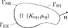 |
Figure 1 Computational domain consisting of an EF with with non-reflecting boundary NNR, excitation boundary ΓEX, sound-hard boundary ΓSH and normal vector n. |
L2 denotes the space of square-integrable functions, and H1 the space of square-integrable functions with square-integrable first derivatives. The additional subscript 0 in (14) denotes zero boundary values.
The modified wave equation (10) is multiplied by the test function p′ and integrated over the subdomains to obtain its weak form
 (15)
(15)
where the acoustic particle acceleration aac emphasized in (10) is substituted and n denotes the normal vector at the boundary. The submatrices resulting from applying the Galerkin procedure are emphasized by the underbraces indicating the coupling between the variables. The underlined variables are vectors of unknowns collecting the nodal degrees of freedom. The boundary term on the excitation boundary ΓEX becomes
 (16)
(16)
The boundary term on the non-reflecting boundary ΓNR is derived in Section 2.4. In case of an adjacent non-dispersive domain, the term becomes an interface condition. When the continuity of the normal acceleration is enforced, the interface term vanishes due to the opposite direction of the normal vectors of the connected domains at the interface.
The ADEs related to the equivalent compressibility (i.e., bulk modulus) read as
 (17)
(17)
 (18)
(18)
and for the ADEs related to the equivalent specific volume (i.e., density) as
 (19)
(19)
 (20)
(20)
2.4 Non-reflecting boundary condition
Analogous to an absorbing boundary condition (ABC), a boundary condition can be established for the TDEF formulation, where outgoing plane waves with normal incidence are fully absorbed. However, due to the dispersive nature of an equivalent fluid, the proposed non-reflecting boundary condition (NRBC) is only exact at a specified target frequency ftr. Hence, the applicability of the introduced NRBC is restricted to problems where the bandwidth of interest is limited. As for the conventional ABC, the knowledge of the plane wave solution for 1D wave propagation in positive x-direction
 (21)
(21)
is exploited, where αtr and βtr denote the real and imaginary part of the complex wavenumber
 (22)
(22)
at the target angular frequency ωtr = 2πftr, respectively. For strongly damped materials, the exponentially decaying term entailed by the imaginary part of the wavenumber βtr becomes relevant and must be considered in the NRBC. Hence, assuming normal incidence of an outgoing wave on ΓNR, the normal derivative computes as
 (23)
(23)
where the relation  was considered. Consequently, the boundary integral on ΓNR in (15) becomes
 (24)
(24)
Unlike for the pressure, where the plane wave solution is exploited, no physical boundary condition can be found for the auxiliary variables. However, this is not required since spatial derivatives only occur in the primary PDE (for the primary variable pac). Hence, the surface normal derivative operator  remains for the auxiliary variables Φv and
  resulting in a bilinear form ∫DNi∇Nj dΓ after applying the Galerkin procedure, where D denotes a coefficient. It is noted that the NRBC is tailored to a specific frequency because the material parameters are evaluated at this discrete angular frequency ωtr. Consequently, the narrow-band NRBC is only applicable for harmonic excitation with target frequency ftrg when transients have vanished. According to [49], multiple narrow-band NRBC operators can be combined to achieve an extended effective bandwidth (Huygens ABC [50]).
In the case of narrow-band excitation, the NRBC can be used to model a thick absorber, where the sound waves are approximately decayed when reaching the end of the absorptive medium. Applying the NRBC allows modeling only a part of the EF, resulting in a reduced number of unknowns and hence computational effort. Typically, the sound propagation in the EF is not of interest, but the impact on the adjacent air domain. In this case, the absorber can be modeled using a few element layers in combination with a narrow-band NRBC resulting in a computational effort comparable to a TDIBC. For oblique incidence, the NRBC is not applicable. In this case, PMLs are necessary, which require special treatment for dispersive material [51].
2.5 Semidiscrete system of equations
Using nodal finite elements, the acoustic pressure as well as the auxiliary variables are approximated as
 (25)
(25)
using FE-Ansatz functions (basis functions) Na according the FEM with n1 being the number of nodes with unknown acoustic pressure (existing in the full domain) and n2 the number of nodes with unknown auxiliary variables (existing in the EF domain only). Applying the Galerkin procedure, we arrive at the following semidiscrete system of equations with the sub-system matrices defined in (15)–(20)
![Mathematical equation: $$ \begin{array}{c}\enspace \underset{\mathbf{M}}{\underbrace{\left[\begin{array}{lllll}\enspace {\mathbf{M}}_{{pp}}\enspace & \mathbf{0}& \mathbf{0}& \mathbf{0}& \mathbf{0}\\ \enspace {\mathbf{M}}_{\mathrm{\Phi }p,j}^C\enspace & \mathbf{0}& \mathbf{0}& \mathbf{0}& \mathbf{0}\\ \enspace {\mathbf{M}}_{\mathrm{\Psi }p,k}^C\enspace & \mathbf{0}& \enspace {\mathbf{M}}_{\mathrm{\Psi \Psi },k}^C\enspace & \mathbf{0}& \mathbf{0}\\ \mathbf{0}& \mathbf{0}& \mathbf{0}& \mathbf{0}& \mathbf{0}\\ \mathbf{0}& \mathbf{0}& \mathbf{0}& \mathbf{0}& \enspace {\mathbf{M}}_{\mathrm{\Psi \Psi },m}^v\enspace \end{array}\right]}}\underset{\stackrel{\dot }{\underline{u}}}{\underbrace{\left[\begin{array}{l}{\underline{\ddot{p}}}^{\mathrm{ac}}\\ {\stackrel{\ddot }{\underline{\mathrm{\Phi }}}}_j^C\\ {\underline{\stackrel{\ddot }{\mathrm{\Psi }}}}_k^C\\ {\underline{\stackrel{\ddot }{\mathrm{\Phi }}}}_l^v\\ {\underline{\stackrel{\ddot }{\mathrm{\Psi }}}}_m^v\end{array}\right]}}+\underset{\mathbf{C}}{\underbrace{\left[\begin{array}{lllll}{\mathbf{C}}_{{pp}}^{\mathrm{NR}}& \mathbf{0}& \enspace {\mathbf{C}}_{p\mathrm{\Psi },k}^C\enspace & \mathbf{0}& \enspace {\mathbf{C}}_{p\mathrm{\Psi },m}^v\enspace +\enspace {\mathbf{C}}_{p\mathrm{\Psi },m}^{\mathrm{NR}}\enspace \\ \mathbf{0}& \enspace {\mathbf{C}}_{\mathrm{\Phi \Phi },j}^C\enspace & \mathbf{0}& \mathbf{0}& \mathbf{0}\\ \mathbf{0}& \mathbf{0}& \enspace {\mathbf{C}}_{\mathrm{\Psi \Psi },k}^C\enspace & \mathbf{0}& \mathbf{0}\\ \mathbf{0}& \mathbf{0}& \mathbf{0}& \enspace {\mathbf{C}}_{\mathrm{\Phi \Phi },l}^v\enspace & \mathbf{0}\\ \mathbf{0}& \mathbf{0}& \mathbf{0}& \mathbf{0}& \enspace {\mathbf{C}}_{\mathrm{\Psi \Psi },m}^v\enspace \end{array}\right]}}\underset{\underline{u}}{\underbrace{\left[\begin{array}{l}{\underline{\dot{p}}}^{\mathrm{ac}}\\ {\underline{\stackrel{\dot }{\mathrm{\Phi }}}}_j^C\\ {\underline{\stackrel{\dot }{\mathrm{\Psi }}}}_k^C\\ {\underline{\stackrel{\dot }{\mathrm{\Phi }}}}_l^v\\ {\underline{\stackrel{\dot }{\mathrm{\Psi }}}}_m^v\end{array}\right]}}\\ +\underset{\mathbf{K}}{\underbrace{\left[\begin{array}{lllll}\enspace {\mathbf{K}}_{{pp}}\enspace +{\mathbf{K}}_{{pp}}^{\mathrm{NR}}& \enspace {\mathbf{K}}_{p\mathrm{\Phi },j}^C\enspace & \enspace {\mathbf{K}}_{p\mathrm{\Psi },k}^C\enspace & \enspace {\mathbf{K}}_{p\mathrm{\Phi },l}^v\enspace +\enspace {\mathbf{K}}_{p\mathrm{\Phi },l}^{\mathrm{NR}}\enspace & \enspace {\mathbf{K}}_{p\mathrm{\Psi },m}^v\enspace +\enspace {\mathbf{K}}_{p\mathrm{\Psi },m}^{\mathrm{NR}}\enspace \\ \mathbf{0}& \enspace {\mathbf{K}}_{\mathrm{\Phi \Phi },j}^C\enspace & \mathbf{0}& \mathbf{0}& \mathbf{0}\\ \mathbf{0}& \mathbf{0}& \enspace {\mathbf{K}}_{\mathrm{\Psi \Psi },k}^C\enspace & \mathbf{0}& \mathbf{0}\\ \enspace {\mathbf{K}}_{\mathrm{\Phi }p,l}^v\enspace & \mathbf{0}& \mathbf{0}& \enspace {\mathbf{K}}_{\mathrm{\Phi \Phi },l}^v\enspace & \mathbf{0}\\ \enspace {\mathbf{K}}_{\mathrm{\Psi }p,m}^v\enspace & \mathbf{0}& \mathbf{0}& \mathbf{0}& \enspace {\mathbf{K}}_{\mathrm{\Psi \Psi },m}^v\enspace \end{array}\right]}}\underset{\stackrel{\dot }{\underline{u}}}{\underbrace{\left[\begin{array}{l}{\underline{p}}^{\mathrm{ac}}\\ {\underline{\mathrm{\Phi }}}_j^C\\ {\underline{\mathrm{\Psi }}}_k^C\\ {\underline{\mathrm{\Phi }}}_l^v\\ {\underline{\mathrm{\Psi }}}_m^v\end{array}\right]}}=\underset{\underline{f}}{\underbrace{\left[\begin{array}{l}{\underline{f}}^{\mathrm{ac}}\\ \underline{0}\\ \underline{0}\\ \underline{0}\\ \underline{0}\end{array}\right]}}\\ \mathrm{for}\enspace j=\mathrm{1,2},\dots,{N}^C,\enspace k=\mathrm{1,2},\dots,{M}^C,\enspace l=\mathrm{1,2},\dots,{N}^v,\enspace m=\mathrm{1,2},\dots,{M}^v,\end{array} $$](/articles/aacus/full_html/2025/01/aacus230096/aacus230096-eq71.gif) (26)
(26)
where 0 and 0 denote a zero matrix and vector of appropriate dimension, respectively. In matrix form, the semidiscrete Galerkin formulation reads
 (27)
(27)
where u collects all nodal unknowns. Observation of the elements of the system matrices reveals, that for the case of a non-locally resonant material having only real poles, no damping term is present in the wave equation itself when no NRBC is used. The only contribution to the damping matrix is given by the ADEs. Therefrom, we can conclude, that energy dissipation is achieved by the ADEs coupled to the wave equation. The imaginary part of complex pole pairs additionally contributes to the stiffness matrix. For time integration of the derived second-order system of ODEs (26), the Newmark-β method is applied.
3 Results
3.1 Study of spatial and temporal convergence
In the following, plane wave propagation in a semi-infinite duct with a strongly damped EF is computed to evaluate the temporal and spatial convergence rates and to demonstrate the effect of the NRBC. The FE mesh of the 2D problem consisting of a 1D arrangement of square elements is depicted in Figure 2. At Γe, a time-harmonic pressure excitation of the form
 (28)
(28)
with a pressure amplitude  Pa and excitation frequency fexc = 1 kHz is imposed. The remaining wall boundary ΓW is assumed sound-hard (vac = 0). Zero initial conditions are considered for the pressure and the auxiliary variables. Hence, the simulation result is expected to match the time-harmonic analytical solution (21) after a sufficiently long simulation time. For the analysis, the fictitious porous material mat1 derived from Yoshida et al. [45] is considered. The EF model exhibits strong damping to emphasize the role of the stiffness term (entailed by the imaginary part of the wave number) and the normal derivatives of the auxiliary variables in the NRBC. The FRFs of the equivalent compressibility
  and specific volume
  are depicted in Figure 3, where the excitation frequency fexc is highlighted. The corresponding rational function approximation coefficients of the EF parameters according to the rational function definition (2a) and (2b) are listed in Table 1.
 |
Figure 2 2D computational domain of a duct considered for the convergence study with a generic mesh consisting of Nel square quadrilateral elements. |
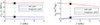 |
Figure 3 Real and imaginary parts of the equivalent compressibility |


Coefficients of the rational function approximation of the equivalent parameters of the fictitious material mat1: residues A, poles α, and constants C∞ and v∞.
In the convergence study, the four different discretization parameters are investigated. The target element size htrg,k determining the spatial discretization is varied as
 (29)
(29)
The initial discretization h0 with htrg,0 = 0.05 m resolving the wavelength λeq = 0.1459 m by approximately 2.9 elements. To verify the NRBC, the duct length L = μl λeq is varied between the maximum length discretization l0 and minimum length discretization l6, where the factor μl ∈ [4, 2, 1, 0.5, 0.25, 0.125, 0.0625] determines the length of the duct. The actually resulting element size hel,k depends on the length discretization l. A comprehensive overview of the resulting actual element sizes is provided by Table 2 for each combination of the spatial discretization h and length discretization l. Three configurations with larger element sizes than the duct length are excluded from the study. In doing so, 33 transient simulations of different element size and duct length were carried out. FE basis functions of polynomial degrees p = 1 (linear elements) and p = 2 (quadratic elements) are considered, denoted as p1 and p2, respectively. Gauss quadrature with the integration order nint = p + 1 is deployed for the numerical integration of the element matrices within the FE procedure [52]. Finally, the time discretization (t0 to t5) of the Newmark time stepping scheme is determined by the time step size Δt = T/μt, where the T denotes the oscillation period and μt ∈ [4, 8, 16, 32, 64, 128] the discretization factor. The initial discretization t0 with a time step size Δt0 = 250 ms resolves one period of oscillation T = 1/fexc = 1 ms by four time steps.
Overview of resulting element sizes hel for the given combinations of length discretizations l0 to l6 and spatial discretization h0 to h5 considered in the convergence study.
The resulting 1D pressure field in the duct is depicted in Figures 4a–4d at selected time steps for the lengths l1, l3, and l5 with discretizations h2, p1, t5.
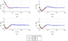 |
Figure 4 1D acoustic pressure field pac(x, t) in a duct filled with homogeneous, sound absorptive material of configurations h2, p1 and temporal discretization t5 for harmonic excitation with fexc. Duct lengths l1, l3, and l5 are considered. The crosses indicate the nodes of the FE mesh. (a) = 0.25 ms ≈ 0.25T; (b) = 1.00 ms ≈ 1.00T; (c) = 2.00 ms ≈ 2.00T; (d) =4.00 ms ≈ 4.00T. |
A strong decay along the x-axis can be observed due to the strong damping in the EF, which essentially wipes out the sound wave over one wavelength λ. The TDEF-based transient simulation matches the analytic solution after about four periods T. The quadratic error
 (30)
(30)
is introduced to quantify the deviation of the transient simulations from the analytical solution. For the computation of the integral, Gauss quadrature with integration order nint = 2p is used, analogous to the FE procedure. The time course of the error ϵΩ(t) is shown exemplarily in Figure 5 for configuration h2, l1, t5 with linear (p1) and quadratic (p2) FE basis functions.
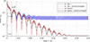 |
Figure 5 Temporal convergence of the quadratic error ϵΩ for time-harmonic excitation of the configuration h2, l1, t5 for linear (p1) and quadratic elements (p2), respectively. After physical transients vanished, the error attributed to the numerical schemes (discretization of time and space) remains. |
The error varies during one period due to the harmonic oscillation of the reference signal  . Therefore, a period-average is computed by applying a moving-mean filter with a sample number corresponding to one period T. The deviation of the transient simulations from the time-harmonic analytic reference decreases non-monotonic due to vanishing transients until the numerical error of the simulation remains. Additionally, a oscillation of the error with a period of approximately 4.3T is superimposed, as indicated in the plot. The subharmonic oscillation is related to the duration of the sound wave inside the duct and therefore depends on the duct length. The remaining error (indicated by the horizontal dashed horizontal lines) can be attributed to the numerical solution.
Figure 6a depicts the quadratic error ϵΩ for the configuration h5, p2, l0 depending on the temporal discretization (t0 to t5). It shows the convergence with second order as expected for the second-order Newmark time integration scheme. Figure 6b reveals that also optimal spatial convergence of order p + 1 is achieved for duct lengths L ≥ λeq (l0 to l2) apart from the highest resolutions where the time discretization prevents the error from falling below 2 × 10⁻⁴ (see Fig. 6a). For a duct length shorter than the wavelength (L < λeq), the NRBC becomes relevant, reducing the order of convergence by one due to the normal derivative of the auxiliary variables (see Sect. 2.4). Obviously, the impact of the NRBC on the error is insignificant for lengths larger than the wavelength because the amplitudes nearly vanish at the non-reflecting boundary ΓNR due to the strong damping in the EF, making the NRBC irrelevant (see Fig. 4).
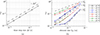 |
Figure 6 Convergence rates of time and space. For the latter, linear (p1) and quadratic (p2) FE basis functions and different duct lengths (l0 to l6) are considered. The dashed grey lines indicate specific orders of convergence. (a) Temporal convergence of configuration h5, p2, l0; (b) Spatial convergence with the finest considered time discretization t5 (Δt = 7.8125 μs). |
3.2 Transient sound propagation in a 2D dissipative domain
Having studied the convergence of the formulation based on harmonic plane-wave propagation, it is now applied to a 2D problem with transient excitation [53]. A smooth pressure pulse defined as (see Fig. 7)
 (31)
(31)
is prescribed at the inner boundary Γe with a radius ri = 0.05 m of the disc, depicted in Figure 8. The transient excitation is chosen according to [40] with the center frequency  , and the coefficients a1 = 1, a2 = −21/32, a3 = 63/768, a4 = −1/512, and βm = 2m−1. The disc with an outer radius of ro = 2.5 m is discretized by approximately 15,800 quadrilateral elements with linear shape functions (p1) and an approximate size of hel = 0.025 m. At the left side of the disc (see Fig. 8), a scatterer with a shape according to [40] is located. At the boundary of the scatterer, the natural sound-hard boundary condition aac · n = 0 is imposed. The dissipative material introduced in Section 3.1 is assigned to the propagation domain (see Tab. 1). At the outer boundary
  , the narrowband NRBC (see Sect. 2.4) is applied. Due to the dispersive nature of an equivalent fluid, the dominating (center) frequency of the excitation signal shifts from fc = 700 Hz to ftr = 40 Hz until the wave reaches the non-reflecting boundary. This target frequency ftr is determined by a preliminary simulation with an extended domain by computing the FFT of a time signal at the position of the boundary r = r0. The NRBC parameters αtr and βtr in (23) are then obtained according to (22) by evaluating the rational function approximations of the equivalent fluid parameters (2a) and (2b) at the target frequency ωtr.
Before the wave reaches the scatterer, the analytic solution on the positive x-axis (y = 0) is given by [53]
 (32)
(32)
where  is the adapted coefficient for satisfying the inhomogeneous Dirichlet boundary condition on Γe at x = ri, and
  denotes the zeroth Hankel function of second kind. The Fourier transformed excitation
  is obtained by applying the fast-Fourier transformation (FFT) to the time signal (31). Computing the inverse FFT of (32) finally yields the semi-analytical solution of (32). The numerical result based on the TDEF formulation is shown in Figure 9 at three selected time steps where the wave has not reached the scatterer. Excellent agreement with the semi-analytical result is achieved apart from the numerical solution at t = 3 ms due to the relatively coarse resolution of the inner boundary Γe, which causes a slight deviation from the semi-analytical solution. Figure 10 shows the instantaneous pressure field at three selected time steps. In the first instance, the wave has not reached the scatterer, while reflections caused by the scatterer are visible in the second instance. To verify the NRBC, the resulting pressure field for a disc with extended radius r0 = 3.75 m is additionally presented in Figure 10b at the time instance t = 36 μs, where the wave pulse has nearly passed the non-reflecting boundary ΓNR. The matching fields inside ΓNR prove the effectiveness of the NRBC for the given application. Note that special care must be taken when setting up the NRBC because the dominating (center) frequency substantially depends on the distance from the source due to the strong dispersive character of the given equivalent fluid. The shift towards smaller frequencies becomes apparent when comparing the changing wavelength in Figure 9. It can be explained by stronger damping at higher frequencies due to an increasing imaginary part of the equivalent compressibility
  and the equivalent specific volume
  (see Fig. 3).
 |
Figure 9 Resulting acoustic pressure along the x-axis of the disc at selected time steps before impingement of the wave at the scatterer. |
 |
Figure 10 Results of 2D wave propagation in a dissipative medium with a sound-hard scatterer at three selected time instances. In (b), the result for an extended domain is shown with an indication of the original size of the disc to verify the NRBC. (a) Acoustic pressure fields at t = 7.5 μs (left) and t = 13.5 μs (right); (b) Acoustic pressure fields at t = 36 μs for the original (left) and extended domain (right). |
4 Conclusions
A time-domain formulation of the equivalent fluid model was derived for the wave equation, allowing the transient analysis of wave propagation in dispersive, sound-absorptive media such as foam. An efficient computation of the arising convolution integral is ensured by applying the auxiliary differential equation method. This method relies on an approximation of the complex-valued frequency response functions of the inverse equivalent bulk modulus (compressibility) and inverse density (specific volume) by a sum of rational functions. The proposed formulation introduces one additional unknown per real or complex-valued pole of the rationals. The ordinary auxiliary equations, indirectly solving the convolution integrals, are coupled to the wave equation, and the auxiliary variables are treated as additional unknowns in the finite element method. Additionally, a narrow-band non-reflective boundary condition for normal incidence is proposed. The derived finite element formulation is implemented and published publicly in openCFS. The validation against the analytical solution for plane wave propagation in a semi-infinite duct showed optimal temporal and spatial convergence rates. Applying it to a 2D wave propagation in an infinite domain with a scatterer further validates the TDEF formulation, including the NRBC. A disadvantage of the proposed NRBC is that it must be tuned to the dominating frequency of the waves passing the non-reflecting boundary. Hence, preliminary knowledge of the frequency content of the wave reaching the boundary is required for dispersive materials because it depends on the distance from the source. Nevertheless, it is favorable regarding computational efficiency because no additional degrees of freedom have to be introduced.
Acknowledgments
We acknowledge the authors of openCFS [54].
Funding
Supported by TU Graz Open Access Publishing Fund.
Conflicts of interest
There are no conflicts to declare.
Data availability statement
The derived finite element formulation is available online through the openCFS repository in GitLab [54], which can be accessed via https://gitlab.com/openCFS/cfs. The data of the convergence study can be found in [53].
References
- S. Schoder, M. Kaltenbacher: Hybrid aeroacoustic computations: State of art and new achievements, Journal of Theoretical and Computational Acoustics 27, 04 (2019) 1950020. [Google Scholar]
- T. Okuzono, T. Otsuru, R. Tomiku, N. Okamoto: Fundamental accuracy of time domain finite element method for sound-field analysis of rooms, Applied Acoustics 71, 10 (2010) 940–946. [CrossRef] [Google Scholar]
- T. Yoshida, T. Okuzono, K. Sakagami: A parallel dissipation-free and dispersion-optimized explicit time-domain fem for large-scale room acoustics simulation, Buildings 12, 2 (2022) 105. [CrossRef] [Google Scholar]
- S. van Ophem, E. Deckers, W. Desmet: Model based virtual intensity measurements for exterior vibro-acoustic radiation, Mechanical Systems and Signal Processing 134 (2019) 106315. [CrossRef] [Google Scholar]
- Y. Cai, S. van Ophem, W. Desmet, E. Deckers: Model order reduction of time-domain vibro-acoustic finite element simulations with admittance boundary conditions for virtual sensing applications, Mechanical Systems and Signal Processing 205 (2023) 110847. [CrossRef] [Google Scholar]
- D. Mayrhofer, M. Kaltenbacher: A new method for sound generation based on digital sound reconstruction, Journal of Theoretical and Computational Acoustics 29 (2021) 2150021. [CrossRef] [Google Scholar]
- H. Wang, J. Yang, M. Hornikx: Frequency-dependent transmission boundary condition in the acoustic time-domain nodal discontinuous Galerkin model, Applied Acoustics 164 (2020) 107280. [CrossRef] [Google Scholar]
- M. Toyoda, S. Ishikawa: Frequency-dependent absorption and transmission boundary for the finite-difference time-domain method, Applied Acoustics 145 (2019) 159–166. [CrossRef] [Google Scholar]
- Y. Özyörük, L.N. Long: A time-domain implementation of surface acoustic impedance condition with and without flow, Journal of Computational Acoustics 5, 3 (1997) 277–296. [CrossRef] [Google Scholar]
- Y. Özyörük, L.N. Long, M.G. Jones: Time-domain numerical simulation of a flow-impedance tube, Journal of Computational Physics 146, 1 (1998) 29–57. [CrossRef] [Google Scholar]
- S. Zheng, M. Zhuang, Verification and validation of time domain impedance boundary condition in lined ducts, AIAA Journal 43, 2 (2005) 306–313. [CrossRef] [Google Scholar]
- J. Bin, M. Yousuff Hussaini, S. Lee: Broadband impedance boundary conditions for the simulation of sound propagation in the time domain, Journal of the Acoustical Society of America 125, 2 (2009) 664–675. [CrossRef] [PubMed] [Google Scholar]
- R. Troian, D. Dragna, C. Bailly, M.-A. Galland: Broadband liner impedance eduction for multimodal acoustic propagation in the presence of a mean flow, Journal of Sound and Vibration 392 (2017) 200–216. [CrossRef] [Google Scholar]
- C. Chen, X. Li: Numerical efficiency analysis of multi-pole time-domain impedance boundary conditions, in 8th European Conference for Aeronautics and Space Sciences, Madrid, Spain, July 1–4, 2019. [Google Scholar]
- R. Fiévet, H. Deniau, E. Piot: Strong compact formalism for characteristic boundary conditions with discontinuous spectral methods, Journal of Computational Physics 408 (2020) 109276. [CrossRef] [Google Scholar]
- F.Q. Hu, D.M. Nark: On the implementation and further validation of a time domain boundary element method broadband impedance boundary condition (AIAA 2022-2898), in 28th AIAA/CEAS Aeroacoustics 2022 Conference, Southampton, UK, June 14–17, 2022. [Google Scholar]
- M. Shur, M. Strelets, A. Travin, T. Suzuki, R. Spalart: Unsteady simulation of sound propagation in turbulent flow inside a lined duct using a broadband time-domain impedance model (AIAA 2020-2535), in AIAA AVIATION 2020 FORUM, Virtual event, 15–19 June, 2020. [Google Scholar]
- M. Shur, M. Strelets, A. Travin, T. Suzuki, P.R Spalart: Unsteady simulations of sound propagation in turbulent flow inside a lined duct, AIAA Journal 59, 8 (2021) 3054–3070. [Google Scholar]
- D. Diab, D. Dragna, E. Salze, M.-A. Galland: Nonlinear broadband time-domain admittance boundary condition for duct acoustics. Application to perforated plate liners, Journal of Sound and Vibration 528 (2022) 116892. [CrossRef] [Google Scholar]
- D. Dragna, P. Pineau, P. Blanc-Benon: A generalized recursive convolution method for time-domain propagation in porous media, Journal of the Acoustical Society of America 138, 2 (2015) 1030–1042. [CrossRef] [PubMed] [Google Scholar]
- H. Wang, M. Hornikx: Broadband time-domain impedance boundary modeling with the discontinuous Galerkin method for room acoustics simulations, in M. Ochmann, V. Michael, J. Fels (Eds.), Proceedings of the 23rd International Congress on Acoustics, 2019: integrating 4th EAA Euroregio 2019, Deutsche Gesellschaft für Akustik, Berlin, Germany, 2019, pp. 779–786. [Google Scholar]
- H. Wang, M. Hornikx: Time-domain impedance boundary condition modeling with the discontinuous Galerkin method for room acoustics simulations, Journal of the Acoustical Society of America 147, 4 (2020) 2534–2546. [CrossRef] [PubMed] [Google Scholar]
- R.J. Luebbers, F. Hunsberger: FDTD for Nth-order dispersive media, IEEE Transactions on Antennas and Propagation 40, 11 (1992) 1297–1301. [CrossRef] [Google Scholar]
- D.F. Kelley, R.J. Luebbers: Piecewise linear recursive convolution for dispersive media using FDTD, IEEE Transactions on Antennas and Propagation 44, 6 (1996) 792–797. [CrossRef] [Google Scholar]
- R. Siushansian, J. LoVetri: Efficient evaluation of convolution integrals arising in FDTD formulations of electromagnetic dispersive media, Journal of electromagnetic waves and applications 11, 1 (1997) 101–117. [CrossRef] [Google Scholar]
- Y. Reymen, M. Baelmans, W. Desmet: Time-domain impedance formulation based on recursive convolution (AIAA 2006–2685), in 12th AIAA/CEAS Aeroacoustics Conference (27th AIAA Aeroacoustics Conference), Cambridge, MA, USA, 8–10 May, 2006. [Google Scholar]
- Y. Reymen, M. Baelmans, W. Desmet: Efficient implementation of tam and auriault’s time-domain impedance boundary condition, AIAA Journal 46, 9 (2008) 2368–2376. [CrossRef] [Google Scholar]
- B. Cotté, C. Blanc-Benon, F. Poisson: Time-domain impedance boundary conditions for simulations of outdoor sound propagation, AIAA Journal 47 (2009) 10. [Google Scholar]
- M. Miller III, S. van Ophem, E. Deckers, W. Desmet: Time-domain impedance boundary conditions for acoustic reduced order finite element simulations, Computer Methods in Applied Mechanics and Engineering 387 (2021) 114173. [CrossRef] [Google Scholar]
- B. Van den Nieuwenhof, J.-P. Coyette: Treatment of frequency-dependent admittance boundary conditions in transient acoustic finite/infinite-element models, Journal of the Acoustical Society of America 110, 4 (2001) 1743–1751. [CrossRef] [PubMed] [Google Scholar]
- Z. Fellah, C. Depollier: Transient acoustic wave propagation in rigid porous media: a time-domain approach, Journal of the Acoustical Society of America 107, 2 (2000) 683–688. [CrossRef] [PubMed] [Google Scholar]
- D.K. Wilson, V.E. Ostashev, S.L. Collier: Time-domain equations for sound propagation in rigid-frame porous media (L), Journal of the Acoustical Society of America 116, 4 (2004) 1889–1892. [CrossRef] [Google Scholar]
- O. Umnova, D. Turo: Time domain formulation of the equivalent fluid model for rigid porous media, Journal of the Acoustical Society of America 125, 4 (2009) 1860–1863. [CrossRef] [PubMed] [Google Scholar]
- D.L. Johnson, J. Koplik, R. Dashen: Theory of dynamic permeability and tortuosity in fluid-saturated porous media, Journal of Fluid Mechanics 176 (1987) 379–402. [Google Scholar]
- Y. Champoux, J.-F. Allard: Dynamic tortuosity and bulk modulus in air-saturated porous media, Journal of applied physics 70, 4 (1991) 1975–1979. [CrossRef] [Google Scholar]
- D. Lafarge, P. Lemarinier, J.F. Allard, V. Tarnow: Dynamic compressibility of air in porous structures at audible frequencies, The Journal of the Acoustical Society of America 102, 4 (1997) 1995–2006. [CrossRef] [Google Scholar]
- J. Zhao, M. Bao, X. Wang, H. Lee, S. Sakamoto: An equivalent fluid model based finite-difference time-domain algorithm for sound propagation in porous material with rigid frame, Journal of the Acoustical Society of America 143, 1 (2018) 130–138. [CrossRef] [PubMed] [Google Scholar]
- J. Zhao, Z. Chen, M. Bao, H. Lee, S. Sakamoto: Two-dimensional finite-difference time-domain analysis of sound propagation in rigid-frame porous material based on equivalent fluid model, Applied Acoustics 146 (2019) 204–212. [CrossRef] [Google Scholar]
- J. Zhao, Z. Chen, M. Bao, S. Sakamoto: Prediction of sound absorption coefficients of acoustic wedges using finite-difference time-domain analysis, Applied Acoustics 155 (2019) 428–441. [CrossRef] [Google Scholar]
- C. Bellis, B. Lombard: Simulating transient wave phenomena in acoustic metamaterials using auxiliary fields, Wave Motion 86 (2019) 175–194. [CrossRef] [Google Scholar]
- A. Alomar, D. Dragna, M.-A. Galland: Pole identification method to extract the equivalent fluid characteristics of general sound-absorbing materials, Applied Acoustics 174 (2021) 107752. [CrossRef] [Google Scholar]
- A. Alomar, D. Dragna, M.-A. Galland: Time-domain simulations of sound propagation in a flow duct with extended-reacting liners, Journal of Sound and Vibration 507 (2021) 116137. [CrossRef] [Google Scholar]
- I. Moufid, D. Matignon, R. Roncen, E. Piot: Energy analysis and discretization of the time-domain equivalent fluid model for wave propagation in rigid porous media, Journal of Computational Physics 451 (2022) 110888. [CrossRef] [Google Scholar]
- H. Wang, M. Hornikx: Extended reacting boundary modeling of porous materials with thin coverings for time-domain room acoustic simulations, Journal of Sound and Vibration 548 (2023) 117550. [CrossRef] [Google Scholar]
- T. Yoshida, T. Okuzono, K. Sakagami: Time-domain finite element formulation of porous sound absorbers based on an equivalent fluid model, Acoustical Science and Technology 41, 6 (2020) 837–840. [CrossRef] [Google Scholar]
- S. Rienstra: Impedance models in time domain, including the extended Helmholtz resonator model (AIAA 2006–2686), in 12th AIAA/CEAS Aeroacoustics Conference, Cambridge, MA, USA, 8–10 May, 2006. [Google Scholar]
- D. Dragna, P. Blanc-Benon: Physically admissible impedance models for time-domain computations of outdoor sound propagation, Acta Acustica united with Acustica 100, 3 (2014) 401–410. [CrossRef] [Google Scholar]
- S.J. Schoder: Aeroacoustic analogies based on compressible flow data, PhD thesis, Technische Universität Wien, 2018. [Google Scholar]
- B. Abdulkareem, J.- Bérenger, F. Costen, R. Himeno, H. Yokota: An operator absorbing boundary condition for the absorption of electromagnetic waves in dispersive media, IEEE Transactions on Antennas and Propagation 66, 4 (2018) 2147–2150. [CrossRef] [Google Scholar]
- J.- Bérenger: On the huygens absorbing boundary conditions for electromagnetics, Journal of Computational Physics 226, 1 (2007) 354–378. [CrossRef] [Google Scholar]
- V. Vinoles, Problèmes d’interface en présence de métamatériaux: modélisation, analyse et simulations, PhD thesis, Université Paris-Saclay (ComUE), 2016. [Google Scholar]
- M. Kaltenbacher: Numerical simulation of mechatronic sensors and actuators: finite elements for computational multiphysics. 3rd edn., Springer, Berlin, Heidelberg, 2015. [Google Scholar]
- S. Schoder, P. Maurerlehner: Metamat 01: A semi-analytic solution for benchmarking wave propagation simulations of homogeneous absorbers in 1D/3D and 2D, ArXiv preprint, 2024. https://doi.org/10.48550/arXiv.2403.03510. [Google Scholar]
- S. Schoder, K. Roppert: openCFS: Open source finite element software for coupled field simulation-part acoustics, ArXiv preprint, 2022. https://doi.org/10.48550/arXiv.2207.04443. [Google Scholar]
Cite this article as: Maurerlehner P. Mayrhofer D. Kaltenbacher M. & Schoder S. 2025. A time-domain finite element formulation of the equivalent fluid model for the acoustic wave equation. Acta Acustica, 9, 3. https://doi.org/10.1051/aacus/2024044.
All Tables
Coefficients of the rational function approximation of the equivalent parameters of the fictitious material mat1: residues A, poles α, and constants C∞ and v∞.
Overview of resulting element sizes hel for the given combinations of length discretizations l0 to l6 and spatial discretization h0 to h5 considered in the convergence study.
All Figures
|
Figure 1 Computational domain consisting of an EF with with non-reflecting boundary NNR, excitation boundary ΓEX, sound-hard boundary ΓSH and normal vector n. |
| In the text | |
|
Figure 2 2D computational domain of a duct considered for the convergence study with a generic mesh consisting of Nel square quadrilateral elements. |
| In the text | |
|
Figure 3 Real and imaginary parts of the equivalent compressibility |
| In the text | |
|
Figure 4 1D acoustic pressure field pac(x, t) in a duct filled with homogeneous, sound absorptive material of configurations h2, p1 and temporal discretization t5 for harmonic excitation with fexc. Duct lengths l1, l3, and l5 are considered. The crosses indicate the nodes of the FE mesh. (a) = 0.25 ms ≈ 0.25T; (b) = 1.00 ms ≈ 1.00T; (c) = 2.00 ms ≈ 2.00T; (d) =4.00 ms ≈ 4.00T. |
| In the text | |
|
Figure 5 Temporal convergence of the quadratic error ϵΩ for time-harmonic excitation of the configuration h2, l1, t5 for linear (p1) and quadratic elements (p2), respectively. After physical transients vanished, the error attributed to the numerical schemes (discretization of time and space) remains. |
| In the text | |
|
Figure 6 Convergence rates of time and space. For the latter, linear (p1) and quadratic (p2) FE basis functions and different duct lengths (l0 to l6) are considered. The dashed grey lines indicate specific orders of convergence. (a) Temporal convergence of configuration h5, p2, l0; (b) Spatial convergence with the finest considered time discretization t5 (Δt = 7.8125 μs). |
| In the text | |
 |
Figure 7 Smooth transient excitation signal according to Bellis and Lombard [40]. |
| In the text | |
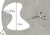 |
Figure 8 Close-up of the FE mesh with the scatterer according to Bellis and Lombard [40]. |
| In the text | |
|
Figure 9 Resulting acoustic pressure along the x-axis of the disc at selected time steps before impingement of the wave at the scatterer. |
| In the text | |
|
Figure 10 Results of 2D wave propagation in a dissipative medium with a sound-hard scatterer at three selected time instances. In (b), the result for an extended domain is shown with an indication of the original size of the disc to verify the NRBC. (a) Acoustic pressure fields at t = 7.5 μs (left) and t = 13.5 μs (right); (b) Acoustic pressure fields at t = 36 μs for the original (left) and extended domain (right). |
| In the text | |
Current usage metrics show cumulative count of Article Views (full-text article views including HTML views, PDF and ePub downloads, according to the available data) and Abstracts Views on Vision4Press platform.
Data correspond to usage on the plateform after 2015. The current usage metrics is available 48-96 hours after online publication and is updated daily on week days.
Initial download of the metrics may take a while.