| Issue |
Acta Acust.
Volume 9, 2025
|
|
|---|---|---|
| Article Number | 49 | |
| Number of page(s) | 13 | |
| Section | Musical Acoustics | |
| DOI | https://doi.org/10.1051/aacus/2025024 | |
| Published online | 06 August 2025 | |
Scientific Article
Sound enrichment of the cristal Baschet by the whiskers
Laboratoire d’Acoustique de l’Université du Mans (LAUM), UMR 6613, Institut d’Acoustique – Graduate School (IA-GS), CNRS, Le Mans Université, Le Mans, France
* Corresponding author: audrey.couineaux@univ-lemans.fr
Received:
11
February
2025
Accepted:
4
June
2025
The cristal Baschet is a musical instrument created during the 50’s by Bernard and Francois Baschet. It is composed of a large number of glass rods arranged in a chromatic scale. Frictional interaction between wet fingers and glass rods triggers self-sustaining vibrations of the resonator, assembly of metal parts and glass rod, which are transmitted to acoustic radiators. The instrument can be equipped with auxiliary elements to modify its timbre. In particular, long thin metal rods called whiskers are commonly added. They act as additional resonators that induce sound enrichment by emphasizing certain higher harmonics. As the manufacturing process of this instrument relies on empirical knowledge, the way whiskers should be tuned to achieve the desired effect is not well known. In this study, modal experimental analysis and numerical modeling are used to understand the dynamic behavior of whiskers and their interaction with the rest of the instrument. First, the simplified structure which is composed of one resonator and one whisker is studied. Experimental measurements are compared with time-domain simulations to gain insight into the role of whiskers and propose tuning guidelines. It is demonstrated that a slow oscillation of the whisker induces a modulation of some specific modes for which the longitudinal and flexural motions are strongly coupled. Such modulation of high order spectral components of the cristal’s sound induces an unusual and characteristic timbre.
Key words: Spectral Enrichment / Time-domain simulation / Modal analysis / Sympathetic resonator
© The Author(s), Published by EDP Sciences, 2025
 This is an Open Access article distributed under the terms of the Creative Commons Attribution License (https://creativecommons.org/licenses/by/4.0), which permits unrestricted use, distribution, and reproduction in any medium, provided the original work is properly cited.
1. Introduction
1.1. Historical context and presentation of the cristal Baschet
The cristal Baschet is a musical instrument created by Bernard and François Baschet in Paris in 1952. This invention is part of a process initiated in 1950, aiming to develop a metal instrument while leveraging the richness and diversity of sounds it enables. This work led to the creation of a wide range of instruments called Structures Sonores [1].
Like other instruments of the Structures Sonores, the cristal Baschet is a modular instrument, designed as assemblies with interchangeable elements. The use of rubbing wet fingers on glass rods attached to threaded shafts to create sound (inspired by the research experiments reported by H. Bouasse [2]) is a common feature across the various versions of the cristal. This evolution is the result of the inventors’ explorations to further develop the instrument: on one hand, to improve the playability of the cristal, and on the other hand, to enhance the efficiency of acoustic radiation. The Baschet brothers collaborated with many musicians, such as Yvonne Lasry, with whom the orientation of the keyboard was modified. The glass rods, initially vertical (Fig. 1a), were then placed horizontally (Figs. 1b and 1c). This completely changed the musician’s gesture and considerably improved ease of playing. Regarding acoustic radiation, they initially used bladders (Fig. 1a), which were later replaced by plates, metal cones, or composite material cones (Fig. 1b).
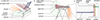 |
Figure 1. (a) Drawing of the first instrument design by the Baschet brothers using friction of glass rods and whiskers, freely colorised and modified from the original drawing [3]; (b) Drawing of a modern cristal Baschet with multiple whiskers, from Structures Sonores Baschet association [1]; (c) Vertical cut of Figure 1b, showing one resonator and its different components. |
In its present form (see Fig. 1b), the cristal Baschet is composed of a large number of glass rods arranged horizontally so as to form a chromatic scale from C1 (65.4 Hz) to C5 (1046.5 Hz). Each glass rod is attached to an assembly consisting of two threaded shafts and a rectangular mass. This assembly, including the glass rod, is called a resonator (see Fig. 1c or beams #1 to #5 in Fig. 2). The present form of the resonator is the result of empirical research by the inventors. The first version of the cristal did not include the rectangular mass and the support threaded shaft (see Fig. 1a). The addition of one threaded shaft and the rectangular mass (named also plongeoir) improved the ease of playing [4] and facilitated the tuning. The mechanical properties of the resonator determine the pitch of the note. All resonators are attached to a thick metal plate called the collector (beam #6 in Fig. 2). Large thin metal panels or cones made of composite materials are connected to the collector to ensure efficient acoustic radiation. These radiating components are not considered in the present study.
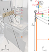 |
Figure 2. (a) Structure R1CW1 on the experimental bench with the position of the accelerometer. Name of the subsystems of R1CW1: 1-rectangular mass (plongeoir), 2-vibrating threaded shaft, 3-support threaded shaft, 4-glass rod,5-connection beam, 6-collector, 7-hanging beam, 8-whisker; (b) Assembly of beams 1 to 8 corresponding to the simplified cristal Baschet (structure R1CW1) used in the FE model. |
The thin and long rods named whiskers, were present right from the start of the cristal’s design (see Fig. 1a). They are usually attached to the collector underneath the highest notes of the instrument (see Fig. 1b) in 3 groups of eight whiskers. They are made of 0.5 mm to 1 mm diameter steel wire with a length, from 60 cm to 150 cm approximately. The way the whiskers are attached can cause them to bend under their own weight (see Fig. 1a). The whiskers were used by the Baschet brothers to create what they called “an echo effect and overtones" [5] and they suggested that whiskers should have different lengths [3].
1.2. Whisker’s effect on the timbre of the cristal
In order to highlight the effect of the whiskers, a structure named R1CW1 is built: it is composed of a single resonator (R1), a single whisker (W1) fixed on a clamped collector (C). The whisker is held in place by a screw on a hanging steel piece attached to the collector (see Fig. 2a).
The structure R1CW1 is played using the nominal gesture: the player applies friction with a wet finger along the glass rod, moving it back and forth. At the end of the excitation, the player stops the friction and holds the glass rod still to prevent free vibrations of the resonator. Two types of gestures are used:
-
soft friction: light contact between the finger and the glass rod, with slow movements of the finger along the glass rod, i.e., low applied normal force F N and low velocity
 of the finger. The approximation of F
N
and
of the finger. The approximation of F
N
and  is illustrated in Figure 3 with FNmax = 0.04 N and
  m/s;
m/s; -
strong friction: firm contact between the finger and the glass rod, with quick movements of the finger along the glass rod, i.e., high applied normal force F N and high velocity
 of the finger. The approximation of F
N
and
of the finger. The approximation of F
N
and  is illustrated in Figure 3 with F
Nmax = 0.4 N and
is illustrated in Figure 3 with F
Nmax = 0.4 N and  m/s;
m/s;
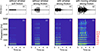 |
Figure 3. Control parameters F
N
and |

The response of the structure R1CW1 under friction excitation is recorded by an accelerometer placed on the back of the collector between the resonator and the whisker (point L). The acceleration at the collector point L can be representative of the sound produced by the instrument, since the collector serves here as a radiating element. This measurement allows for an easy comparison with a time-domain simulation.
As a reference configuration, the structure without whisker (R1C) is played with the two types of gesture. The acceleration recorded at point L and the associated spectrogram are shown in Figures 4a to 4d. The response exhibits a perfect harmonic spectrum, resulting from the periodic self-sustained oscillations induced by friction [6]. The fundamental frequency noted H1 corresponds to a particular mode of the structure for which the deformation is located in the “vibrating threaded shaft" (see mode shape J in Fig. 5). The n-harmonics are noted Hn = nH1. In the case of soft friction, the response is relatively close to a pure tone with the dominance of the two first harmonics (H1 and H2). In the case of strong friction gesture, the produced sound is richer. The vibration stops suddenly at the end of the fourth movement of the finger, with no sustain.
Then, one whisker is added to the structure (R1CW1) and a strong friction gesture is applied. The response is shown in Figures 4e and 4f. Compared to the reference configuration, the second and fourth harmonics are now amplified. Additionally, these frequencies exhibit a long sustain at the end of the fourth movement of the finger. This spectral enrichment and sound sustain on specific harmonics is the first sound effect generated by the whisker. It is hereafter referred to as sympathetic vibration effect. It should be noted that the length of the whisker has been tuned to achieve this effect: a whisker with a different length would give a response similar to that in Figure 4d. The manner in which the tuning is done will be developed in Section 3.
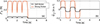 |
Figure 4. Measured acceleration at collector point L during playing situation on the structure composed of one resonator, one collector (a to d), and with one tuned whisker (e to h). In (g and h), the whisker is moving slowly with large amplitude. On the first line are the acceleration versus time; on the second, line the associated spectrogram. The acceleration amplitude is normalized by the maximum amplitude measured. The fundamental frequency is H 1 = 191 Hz. The sounds are available in the complementary materials. |
In a real playing situation, when the musician plays with strong attacks, the lowest global modes of the entire structure may be excited by the back-and-forth motion of the fingers. The lowest modes of the whiskers (typically in the range of Hertz) can also be excited, resulting in low-frequency oscillations in the whiskers, which produce a distinctive sound effect. This phenomenon is reproduced on the structure R1CW1 by initiating a large oscillating motion of the whisker while the instrument is being played. The result is shown in Figures 4g and 4h. The produced sound is quite unusual compared to those commonly produced by musical instruments. The slow oscillation of the whisker induces a frequency modulation occurring between 1900 and 2400 Hz, which is clearlyvisible in the spectrogram. This modulation effect can also be observed at higher frequencies, around 4500 Hz.
The conditions under which these two effects occur are not well known or described by the instrument maker, making the whiskers tuning process difficult. The aim of this article is to understand the conditions in which the sympathetic vibration and modulation effects occur and to provide tuning guidelines from the instrument maker’s perspective.
In order to address this issue, a physical model is developed in Section 2. The proposed model builds on the previous work [7], which describes the interaction between a wet finger and a single resonator of the cristal Baschet. In Section 3, the model will be used to explain the sympathetic vibration effect. In Section 4, the modulation effect at high frequencies will be explained and described.
2. Physical model of a resonator equipped with whisker
Because the cristal Baschet is a little-studied musical instrument [7, 8], the developed physical model is strongly inspired by bowed string models [9, 10], using similar parameters to model the finger like a bow [11]. The modal formulation, commonly employed in the literature to model the dynamic behaviors of strings [12, 13] or bars [14], is also applied in our model. The sound produced by the cristal Baschet arises from friction-induced vibrations, various examples of friction-induced vibrations are presented in Akay’s work [15]. Lot of friction models exist [16], the friction model used in the bowed string [12, 17] allows to describe the stick-slip phenomenon, and are implemented in our model with adaptations for finger contact [18]. The physical model for the cristal Baschet and implementation of the time-domain simulations are discussed in the next paragraphs.
2.1. Equations for the friction induced vibrations
The physical model represents the structure R1CW1 and aims to highlight the spectral enrichment caused by the whiskers. This model is based on the minimal cristal model [7], which describes the interaction between the musician’s finger and an isolated resonator. In this adapted model, the resonator is no longer isolated but attached to the collector, with a whisker added. Therefore, the assumptions regarding the interaction between the finger and the glass rod remain similar to those in the previous model and are briefly summarized below.
The following assumptions are made regarding the musician’s gesture: The rubbing finger is considered as a rigid body which means its own dynamic behavior is ignored. The finger moves along the glass rod in the x-axis with a velocity denoted by  . This uniaxial movement provides a simplified representation of the musician’s gesture. The interaction between the finger and the glass rod is modeled by a point force since the contact surface is assumed to be very small compared to the length of the rod. The contact point is denoted by C (see Fig. 2b) and the normal force (along the z-axis) applied by the finger on the rod is denoted by FN. In order to simplify the time-domain simulation, the point C is considered constant over time. These assumptions simplify the musician’s gesture using two parameters (FN and
  ). In a real playing situation, there are various ways to execute a gesture to express musicality. For example, the cristalist can pinch and grab the glass rod more or less firmly using multiple fingers.
The frictional interaction is based on the following assumptions. The interaction between the finger and the glass rod is described by a friction law that distinguishes between sticking and slipping states. This law expresses a relationship between the frictional force F
T
exerted on the glass rod and the relative velocity  between the glass rod and the finger. In a slipping state, the frictional force F
T
is proportional to the normal force F
N
and acts in opposition to the relative motion between the glass rod and the finger. The friction coefficient μ is assumed to depend on the relative velocity
between the glass rod and the finger. In a slipping state, the frictional force F
T
is proportional to the normal force F
N
and acts in opposition to the relative motion between the glass rod and the finger. The friction coefficient μ is assumed to depend on the relative velocity  . In a sticking state, the maximum frictional force is characterized by a static friction coefficient μ
s
(see more details about the friction curve in the Appendix A). The parameters of the friction law are considered constant over time. In real playing conditions, the amount of water on the glass rod decreases with time, leading to changes in the characteristics of the friction law. Consequently, the musician must periodically “reload” by dipping their fingers into a tank of water.
. In a sticking state, the maximum frictional force is characterized by a static friction coefficient μ
s
(see more details about the friction curve in the Appendix A). The parameters of the friction law are considered constant over time. In real playing conditions, the amount of water on the glass rod decreases with time, leading to changes in the characteristics of the friction law. Consequently, the musician must periodically “reload” by dipping their fingers into a tank of water.
Concerning the structure R1CW1 by itself, we consider the following assumptions. The structure R1CW1 is considered a linear and time-invariant structure, allowing its dynamics to be described by a set of eigenmodes. In practice, to model the modulation effect induced by the whisker, this assumption is considered for a short period of time (see Sect. 4). Its motion is restricted to the (x, z)-plane (see Fig. 2b) that corresponds to the symmetry-plane of the structure, in order to simplify the studied system. The motion is described by an equation of the form:

where x(t) is the [N S , 1] displacement vector, associated to the N S degrees of freedom describing the structure, and f(t) is the [N S , 1] force vector applied (see in the Appendix A the detailed expression of this vector). M S , C S and K S are respectively the [N S , N S ] mass, damping and stiffness matrices. This equation is a rewrite of the equation (1) of [7].
The displacements x(t) are expressed using a modal expansion involving N modes (N ≤ N S ), and take the form x(t)=Φ q(t), where q(t) and Φ are respectively the [N, 1] vector of modal coordinates and the [N s , N] modal matrix (see more details about the expression of the vectors in the Appendix A). The mode shapes Φ k (columns of matrix Φ) are determined from the associated conservative system (C S = 0). The natural frequencies and damping ratios are determined from the complex eigenvalues of the dissipative problem, for which damping values in the various subsystems are different and taken into account by considering complex Young’s modulus E = E 0(1 + j η) (loss factors η listed in Tab. 1).
The orthogonality of conservative modes allows the equation of motion to be written in the modal basis as:

where M = Φ T M s Φ = diag(m k ) is the [N, N] modal mass matrix, C = diag(2ξ k ω k m k ) the [N, N] modal damping matrix involving damping ratios ξ k , K = Φ T K s Φ = diag(m k ω k 2) the [N, N] modal stiffness matrix involving the natural angular frequencies ω k . These modal parameters can be obtained numerically, as described in the Section 2.3.1.
2.2. Time-domain simulations
We aim to account for the whisker effect as observed experimentally. To do so, we consider the structure R1CW1 (resonator, collector, whisker) characterized by its modal base and a frictional contact. The time-domain simulations aim to describe the occurrence of self-sustained oscillations in a playing situation and to qualitatively reproduce the two whisker effects. The method used for performing the simulation is briefly described, as it has already been detailed in previous work [7].
This method is based on an explicit numerical scheme adapted from Demoucron [12] to iteratively solve the modal equations (Eq. (2)). The solution is computed at discrete time steps t
i + 1 = t
i
+ Δt, where Δt is the sampling period. When Δt is sufficiently small compared to the characteristic time of the system’s dynamics, the frictional force can be considered constant over the interval ]t
i
, t
i + 1]. The sampling frequency is set to 48 kHz, which results in a Δt of approximately 21 μs. As a comparison, the highest natural frequency in the modal basis considered here is about 2500 Hz, characteristic time (period) of 0.4 ms. Consequently, the right-hand side of the modal equations (Eq. (2)) remains constant during this interval. An analytical solution can then be used to calculate the state of the system at time t
i + 1, described by the set of modal coordinates q(t
i + 1) and their derivatives  , knowing its state at time t
i
and the constant modal forces f(t
i + 1). This leads to the following explicit recurrence relation:
, knowing its state at time t
i
and the constant modal forces f(t
i + 1). This leads to the following explicit recurrence relation:
The expressions of the matrices A 11, A 12, A 21, A 22, B 1, and B 2 are provided in [7].
To enable a qualitative comparison between the model and experimental measurements, the response of the modeled structure is observed at point L, located approximately at the same position as the accelerometer (equidistant from the resonator and the whisker attachment). Additionally, since the numerical scheme provides displacement or velocity, the acceleration is obtained through numerical differentiation.
The time-domain simulations are performed under two typical gestures, referred to as soft and strong friction. The control parameters used to model these two gestures are shown in Figure 3. The normal force FN and the velocity of the finger  vary over time and describe five steps of finger movement (pushing–pulling–pushing–pulling–stop). When the velocity
  , the movement is referred to as pulling, and when
  , it is called pushing. The transition between the two movements is short and is accompanied by a relaxation of the normal force F
N
. The finger then stops at t = 4 s, but the force remains non-zero for 0.1 s to ensure that the resonator vibrations stop as well. The force and absolute velocity are higher for the strong friction case compared to the soft friction case.
, it is called pushing. The transition between the two movements is short and is accompanied by a relaxation of the normal force F
N
. The finger then stops at t = 4 s, but the force remains non-zero for 0.1 s to ensure that the resonator vibrations stop as well. The force and absolute velocity are higher for the strong friction case compared to the soft friction case.
2.3. Modes of the structure R1CW1
2.3.1. Beam finite element model
In this work, the modes of the structure R1CW1 are obtained through a numerical approach, enabling useful parametric analyses. The numerical modal analysis is conducted using a in-house finite element model composed of an assembly of beam elements, as the majority of the structure’s elements can be modeled by beams. The elements considered account for bending (under Euler–Bernoulli assumptions) as well as tension-compression. Each element is characterized by an elementary stiffness and mass matrix, with expressions derived from [19]. The mesh describes a regular pattern with a mesh size of 1 mm, obtained with a convergence study up to 2500 Hz.
The cristal is divided in beam substructures, ranging from beams #1 to #8. The resonator is described by beams #1 to #5, the collector by beams #6 and #7 and the whiskers beam #8. The geometry and material of each beam are derived from the actual dimensions and materials of the structure R1CW1 (see Fig. 2) and are respectively presented in Tables 2 and 1. Usual values of Poisson’s ratio are considered. The Young’s modulus of steel [21], aluminum and glass [20] are adjusted in order to minimize the frequency deviation between numerical and experimental eigen-frequency of the main mode (see mode shape J in Fig. 5). The frequency of this mode corresponds to the fundamental frequency of the produced sound under friction (fnum = 186 Hz and fexp = 191 Hz). Regarding the geometry, the connection between the resonator and the collector is arranged differently from the experimental arrangement to comply with the restriction of motion in the (x, z)-plane. The threaded rods are modeled with a uniform cross-section, but with a diameter slightly smaller than the actual outer diameter of the threads. The bolts are not included in the model. The connections between beams are considered perfect: the two beams involved in each connection share a common node, ensuring equal displacements and rotations at that node. Clamped boundary conditions are applied at one extremity of the collector (point B see Fig. 2b), the other boundary conditions are free.
Dimensions of the beams used in the FE model.
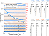 |
Figure 5. Eigenfrequencies of one-note cristal with whisker as a function of whisker length L w . The color and marker type give the modal classification (resonator mode, whisker mode or global mode). Black markers with associated letter indicate mode shape illustrations. The gradient towards light orange on the mode shape reflects the deformation along x on the whisker, highlighting the whisker’s longitudinal mode (N, O, P, Q). |
2.3.2. Variation of the modal parameters
2.3.2.1. Effect of whisker length
A parametric study is conducted on the length of the whisker, denoted L w , as this parameter is the primary criterion used by makers to obtain the sound effects induced by the whisker. The length range studied is reduced to the one used by the instrument maker (0.6 m to 1.5 m). For each length, the modes are calculated using the finite element model.The eigenfrequencies are shown in Figure 5 in the chosen frequency range (from 0 to 2500 Hz). This range is sufficient to observe the two sound effects induced by the whisker in the next sections (Sects. 3 and 4). The modes are then classified into several categories using a Kinetic Energy Ratio (KER) criterion [22], defined as the ratio of the kinetic energy of a substructure (resonator, whisker, or collector) to the total kinetic energy of the structure. When at least 95% of the kinetic energy of a mode is localized within a substructure, it is considered a local mode (of the resonator, whisker, or collector). The remaining modes are classified as global.
Figure 5 presents this parametric study with the classification. The first observation is that no local modes of the collector are observed in this frequency range. A plausible reason for this is that any deformation of the collector systematically causes displacement of the resonator and the whiskers, preventing the kinetic energy from being confined within the collector. An illustration of mode shapes obtained for other categories of modes is presented on the side of the figure. In particular, one local mode of the resonator (J) and two local modes of the whisker (K and L) are shown.
The frequencies of the resonator modes and the majority of global modes vary very little as the length of the whisker increases (see mode M or J in Fig. 5). The frequencies of the whisker bending modes vary with length according to the law f n ∝ 1/L 2, this stems from the known expression of the modes of a clamped-free beam. This can be observed in Figure 5 by examining the trajectory of the orange tiny dots. A trajectory with f n ∝ 1/L is also observed for some modes categorized as global. When the corresponding mode shape is examined, it is noted that it corresponds to the longitudinal mode of the whisker coupled with the rest of the system, this mode plays a major role in the whisker’s effect analysis. The shape evolution of this mode illustrated by mode shape for 4 different lengths: mode shape N, O, P and Q, corresponding to the whisker length L w = 0.85, 1.07, 1.26 m and 1.45 m respectively. The longitudinal deformation of the whisker is highlighted by a gradient of orange. This gradient represents the deformation along the x-axis in the whisker (see Fig. 5).
2.3.2.2. Effect of whisker curvature
In a playing situation, when the musician applies significant pressure on the glass rods, the back-and-forth motion of the finger can induce a rocking motion of the instrument on its feet. This movement then induces oscillations of the whisker, which visually correspond to the first mode of the cantilever beam. The frequency of this first mode is very low (on the order of Hz) compared to the playing frequency (here, 191 Hz). The dynamics of the whisker oscillations are therefore very slow compared to the dynamics of the system involved in the self-oscillations resulting from friction. To take into account this phenomenon in the model, a reasonable hypothesis is to impose a quasi-static oscillation of the whisker during the simulation. Practically, this is achieved by regularly updating the modal basis of the system, in which the shape of the whisker varies. The whisker then vibrates around a position w(x, t), which slowly varies over time, as given by

where ψ(x) is a function that defines the shape of the oscillation, which is supposed to be given by the first mode of a cantilever beam:
with β 1 = 1.875/L w and σ 1 = 0.734 described in [23].
A condition of constant length is added to avoid artificially elongating the whisker by imposing this position. In practice, this amounts to evaluating equation (4) for x ∈ [0, x max], where x max is determined such that
Before the time-domain simulations, we focus specifically on potential modifications of the modal basis induced by the curvature of the whisker, by calculating the modes for fixed values of α. To achieve this, α is varied between −0.4 and 0.4, resulting in the positions shown in Figure 6. This figure illustrates the shortening along x (i.e. xmax ≤ Lw) that results from the condition of constantlength.
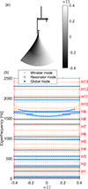 |
Figure 6. (a) Curvature factor illustrated from α = −0.4 (black) to α = 0.4 (white). (b) Eigenfrequencies of the simplified cristal as a function of the curvature factor induced by the first whisker bending mode. |
Figure 6 shows the variation of modal frequencies as a function of α. The same classification of modes as in Figure 5 is used. The frequency of most modes does not change significantly with curvature. However, significant changes occur in a narrow frequency range slightly above 1500 Hz. This corresponds to the first longitudinal mode of the whisker, which couples with various bending modes due to curvature. The greater the curvature, the higher the frequency of this coupled mode. This behavior is symmetrical with respect to zero curvature. Additionally, some modes, whose frequencies remain unchanged with curvature, change classification and transition to the group of global modes. This indicates modal hybridization, which occurs when two modes are close in frequency, a phenomenon known as mode veering [24].
3. Sympathetic vibrations induced by the whisker
In order to highlight the sound effect induced by the whisker, time-domain simulations are performed for several whisker lengths. The curvature of the whiskers is not taken into account in this section. The time-domain simulations allow helping to identify the key parameters necessary for this phenomenon for a qualitative reproduction of the experimentally observed effect.
3.1. Frequency coincidence between whisker mode and harmonics
The whisker’s effect has been described as spectral enrichment and sound sustain on specific harmonics. However several factors can contribute to spectral enrichment and sound sustain, some related to the whisker and others to the musician’s control parameters. This section examines these factors to emphasize the sound effect induced by the whisker and the conditions required to achieve it.
3.1.1. Spectral enrichment due to the excitation
Figure 7 shows the system’s response at point L under friction excitation: the first three columns present the response under soft friction (FN = 0.04 N and  m/s, see Fig. 3), and the last three columns show the response under strong friction (F
N = 0.4 N and
m/s, see Fig. 3), and the last three columns show the response under strong friction (F
N = 0.4 N and  m/s).
m/s).
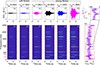 |
Figure 7. Time-domain simulations for two types of control parameters soft friction (a to f) and strong friction (g to l) and 3 different whisker lengths: L w = 0 m (a, b, g, h), L w = 1.20 m (c, d, i, j) and L w = 1.26 m (e, f, k, l). The acceleration of the cristal at the L-point is calculated, the corresponding spectrogram is plotted. (m) The frequency tranfer-function, from the FE model, at the whisker M-point for two whisker lengths L w = 1.2; 1.26 m. The fundamental frequency is H 1 = 186.3 Hz. The acceleration amplitude is normalized by the maximum amplitude calculated. |
When the friction gesture is strong (Figs. 7g to 7l), the spectrum exhibits more harmonics with significant amplitude than under soft friction (columns 1, 2, 3). However, this spectral enrichment occurs regardless of the whisker length. It is a characteristic feature of the stick-slip regime: when the normal force is higher, the sticking phase lasts longer in each period, requiring more harmonics to describe the signal. This phenomenon of spectral enrichment has already been observed in bowed string instruments [25] and can be seen experimentally (Figs. 4).
3.1.2. Spectral enrichment due to the whisker
Time-domain simulations are performed for three different whisker lengths: L w = 0, corresponding to the reference system without whisker, L w = 1.2 m, representing an arbitrary whisker length with no particular effect, and L w = 1.26 m, corresponding to a tuned whisker where a specific sound effect is observed.
The spectrograms show that the responses of the structure without a whisker or with an untuned whisker are very similar. In contrast, for a tuned whisker, the spectrogram in the third column exhibits a clear amplification of the fifth harmonic (H5). When examining the transfer function, calculated with the FE model, with excitation and response at point M, located on the whisker, it is observed that a pronounced resonance coincides with the frequency of the fifth harmonic (H5) in the case of the tuned whisker (magenta curve), which is not the case for the arbitrary length (blue curve). This suggests that a natural frequency of the whisker must coincide with a harmonic to produce a sound enrichment effect.
3.1.3. Sustain on specific harmonics due to whisker
The sound sustain due to the L
w
= 1.26 m whisker is also observed on the same harmonic H5 and is directly linked to the sympathetic vibrations described above. To highlight this sound sustain, a sudden stop of the resonator vibration at the end of the gesture is simulated. This is achieved by maintaining a high normal force F
N
while the finger speed  is rapidly set to zero (see Fig. 3). In the spectrograms, a clear stop of the fundamental frequency can be observed at t = 4 s (see Fig. 7).
This sudden stop is also performed experimentally by the musician, and the sustain effect is similar (see Fig. 4). However, the simulated response also exhibits a sustain of non-harmonic components, which is due to the transient response of weakly damped modes once the periodic regime ends. This phenomenon arises because we did not attempt to precisely adjust the varied damping rates of the numerous modes in the R1CW1 structure to match the experimental damping ratios. Instead, we accounted for structural damping in our model (see Tab. 1), which cannot accurately represent the damping effects caused by the numerous joints and assemblies.
In conclusion, for a specific length (Lw = 1.26 m), a sympathetic vibration effect induced by the whisker is observed, marked by the amplification of a harmonic (spectral enrichment) and a pronounced sustain of this component during the free response phase, at the end of the self-sustained oscillations. This effect results from a frequency coincidence between a harmonic and a whisker mode. The high modal density of the whisker (see Fig. 5) tends to favor such coincidences. However, this condition alone is not sufficient, as there are cases where a whisker natural frequency coincides with a harmonic without producing this effect, for example in Figure 5, at Lw = 0.64; 1.05, 1.47 m whisker modes coincide with the harmonic (H5). Therefore, an additional condition is necessary to achieve the desired effect.
3.2. Importance of collector vibrations in achieving the whisker effect
To quantify the impact of the collector on the whisker’s sympathetic vibration effect, the transfer mobility between the resonator (point C, see Fig. 2) and the collector (point L) is analyzed: The transfer mobility is calculated for each whisker length and is presented in a map visible in Figure 8a. The influence of the whisker length on the amplitude of mobility is very important. Consequently, for specific frequencies (harmonics of the sound played), a significant amplification of sympathetic effect of the whiskers can be obtained if the length is adjusted. At the frequency of the H5 harmonic(horizontal line in Fig. 8), a maximum amplitude of mobility is reached for the length Lw = 1.26 m, which corresponds to the whisker length that produces a sympathetic vibration effect. At the frequency of the H3 harmonic, mobility is high but does not vary with the whisker length. Therefore, the potential spectral enrichment due to this particular harmonic does not depend on the whisker, as observed in the spectrograms in Figure 7. Conversely, the amplitude of the transfer mobility for certain harmonics, such as H2, H4, or H11, is not affected by changes in whisker length. To achieve the whisker effect at these harmonics, modifications to the whisker’s diameter or its coupling with the collector should be explored.
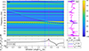 |
Figure 8. (a) Amplitude of the transfer mobility between the resonator (point C) and the collector (point L) |V L z /F C x | versus frequency and whisker length L w ; (b) Transfer mobility for the specific whisker’s length L w = 1.26 m in magenta and L w = 1.20 m in blue as a function of the frequency, these lengths are indicated by dashed vertical lines in (a); (c) Transfer mobility amplitude as a function of whisker length at a specific frequency H5. |
In conclusion, the effect of sympathetic vibration induced by the whiskers requires two criteria: first, a frequency coincidence between a harmonic and a whisker mode, and second, a significant amplitude of transfer mobility between the resonator and the collector at this frequency. This explains the difficulty for instrument makers in achieving proper tuning of the whiskers.
4. Modulation of the sympathetic vibration by time-varing of the whisker’s parameters
Other phenomena were observed experimentally (see Fig. 4h), notably modulations of high-frequency components of the spectrum when the whisker oscillates, i.e. when its curvature evolves slowly.
We showed in Section 2.3.2.2 that the curvature of the whisker affects the frequency of its longitudinal mode, which is coupled with transverse modes (see Fig. 6). When this curvature α changes over time, the frequency of this mode also evolves and can thus meet the condition of frequency coincidence with a harmonic, as discussed in the previous section.
In the time-domain simulation, the α(t) amplitude is supposed to vary slowly according to:

where α 0 is a constant coefficient used to represent the initial (static) curvature and α m is a coefficient that determine the amplitude of the slow oscillations at angular frequency Ω. This angular frequency corresponds to the eigen-frequency of the first bending mode of the whisker.
To examine the impact of different slow variations in curvature, time simulations are performed. For these simulations, the control parameters used are those characteristic of strong friction and the whisker length is set to 0.8 m. This specific length is chosen in order to emphasis the effect of modulation. To account for the slow oscillation of the whisker defined by equation (4), a piecewise time resolution is implemented: the simulation is divided into several successive time windows, each lasting 20 ms, during which the curvature α remains constant (the modal basis thus does not change during this time window). At the start of each subsequent time window, the curvature of the whisker is updated, along with its modal basis. The initial conditions for each new window are the modal displacements and velocities from the end of the previous window.
The results of various time simulations are shown in Figure 9. A case without curvature variation is presented in the Figures 9a to 9c, serving as a reference case. The different harmonics generated by the effect of friction can be observed, as previously noted in Section 3. Variousscenarios are then proposed to simulate the curvature variations that the whisker might undergo if it slowly oscillates in its first mode around 1.1 Hz (see Figs. 9d to 9l). When the curvature changes, a modulated high-frequency component appears. This modulation is independent of the fundamental frequency, which remains unchanged. The modulation patterns visible in the spectrograms are directly correlated with the parameter α given by equation (7), which controls the whisker modes. In the Figures 9h and 9i, the modulation occurs twice in a cycle due to the symmetry of eigenfrequencies with α = 0 highlighted in Figure 6. In other words, the modes associated with a curvature state α remain unchanged when α is replaced by −α which can give ever more complicated modulation pattern when α oscillating around zero but not centered in zero like the Figures 9j to 9l.
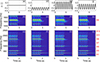 |
Figure 9. Time-domain simulations for four different type of curvature α: (a, b, c) α 0 = 0 and α m = 0, (d, e, f) α 0 = −0.25 and α m = 0.1, (g, h, i) α 0 = 0 and α m = 0.3, (j, k, l) α 0 = −01 and α m = −0.2; The α parameter versus time, the spectrogram of the acceleration of the point L and the zoom view of the spectrogram. The acceleration amplitude is normalized by the maximum amplitude calculated. The fundamental frequency is H 1 = 186.3 Hz. |
The high-frequency modulation thus corresponds, for all three scenarios, to the changes in the natural frequency of the whisker’s longitudinal mode, which couples with different neighboring bending modes due to the time-varying curvature.
5. Conclusion
The cristal Baschet is a friction-based instrument, where various sound-enhancing accessories, such as whiskers, can be added to enrich the produced sound. A physical model was developed to describe the phenomenon of spectral enrichment induced by the whiskers. This model accounts for the dynamics of a simplified cristal structure, including a single resonator, a collector, and a single whisker. Parametric studies on whisker length and curvature were conducted to understand the influence of these parameters on the producedsound.
The spectral enrichment achieved by adding a whisker is a form of sympathetic vibration that occurs under very specific conditions. These conditions involve a precise frequency coincidence between a harmonic of theself-sustained vibrations generated by friction and the eigenfrequency of a whisker. In addition, the value of transfer mobility between the collector and the friction point enables the transfer of the sympathetic vibration, allows the device to be used. The simultaneous occurrence of these conditions is relatively rare compared to the large number of modes in the whisker.
This finding suggests that adding multiple whiskers of varying lengths could extend this spectral enrichment to several harmonics, as it increases the likelihood of achieving a frequency match between a harmonic and a whisker mode because of the high modal density of the assembly. This aligns with practices by cristal makers. Modifying the position of the whisker on the collector and the attachment conditions are potential strategies for improving the transfer of sympatheticvibrations.
Modulation phenomena due to changes in whisker curvature were observed experimentally and explained using the model. This modulation is linked to the shift in the natural frequency of the whisker’s longitudinal mode due to its curvature. When this frequency modulates and crosses a harmonic generated by friction, the sympathetic vibration phenomenon is triggered.
This study demonstrates how a physical model of the instrument can be adapted and used to understand the spectral enrichment and modulation effects provided by whiskers. The analysis sheds light on the choices made by makers and offers guidance for tuning whiskers to control this effect.
Supplementary material
Measured acceleration of the structure without whisker under soft friction (Fig. 3ab).
Measured acceleration of the structure without whisker under strong friction (Fig. 3cd).
Measured acceleration of the structure with whisker under strong friction (Fig. 3ef).
Measured acceleration of the structure with moving whisker under strong friction (Fig. 3gh).
Access hereAcknowledgments
The authors expressed their gratitude to the ENSIM students (Engineering school of Le Mans University) G. Deneil, V. Dorey, A. Laboulfie, S. Lemieux, L. Tricaud for the first experimental explorations, and also to M. Dauxais, intern at Le Mans University, for the first numerical explorations.
Conflicts of interest
The authors declare that they have no conflicts of interest.
Data availability statement
The data are available from the corresponding author on request.
References
- Association Structure Sonore Baschet: http://baschet.org/. Accessed:2024-09-04. [Google Scholar]
- H. Bouasse: Verges et plaques, cloches et carillons. Delagrave, Paris, 1927. [Google Scholar]
- F. Baschet, B. Baschet: Organologie des structures Sonores Baschet. Vol. 1 and 2. Self-publisher, 1985. [Google Scholar]
- F. Baschet: Journal d’une recherche acoustique 1953 á 1963. Vol. 1. Self-publisher, 1963. [Google Scholar]
- F. Baschet: The Sound Sculptures of Bernard and François Baschet. Edicions de la Universistat de Barcelona, 2017. [Google Scholar]
- A. Jenkins: Self-oscillation. Physics Reports 525, 2 (2013) 167–222. [Google Scholar]
- A. Couineaux, F. Ablitzer, F. Gautier: Minimal physical model of the cristal Baschet. Acta Acustica 7 (2023) 49. [CrossRef] [EDP Sciences] [Google Scholar]
- F. Gautier, J.-L. Le Carrou, A. Elmaian, F. Bousquet: Acoustics of the cristal Baschet, in: 20th International Symposium on Music Acoustics, Sydney and Katoomba (Australia), 2010. [Google Scholar]
- T.D. Rossing: The Science of String Instruments. Springer, 2010. [Google Scholar]
- A. Chaigne, J. Kergomard: Acoustique des instruments de musique (Acoustics of Musical Instruments) (2e édition revue et augmentée). Belin, 2013. [Google Scholar]
- J.C. Schelleng: The bowed string and the player. The Journal of the Acoustical Society of America 53 (1973) 26–41. [Google Scholar]
- M. Demoucron: On the control of virtual violins Physical modelling and control of bowed string instruments. PhD thesis, Université Pierre et Marie Curie – Paris VI; Royal Institute of Technology, Stockholm, 2008. [Google Scholar]
- V. Debut, J. Antunes, O. Inácio: Linear modal stability analysis of bowed-strings. The Journal of the Acoustical Society of America 141, 3 (2017) 2107–2120. [Google Scholar]
- O. Inácio, L. Henrique, J. Antunes: Simulation of the oscillation regimes of bowed bars: a non-linear modal approach. Communications in Nonlinear Science and Numerical Simulation 8, 2 (2003) 77–95. [Google Scholar]
- A. Akay: Acoustics of friction. The Journal of the Acoustical Society of America 111 (2002) 1525–1548. [Google Scholar]
- F. Marques, P. Flores, J.-C.P. Claro, H.M. Lankarani: Modeling and analysis of friction including rolling effects in multibody dynamics: a review. Multibody System Dynamics 45 (2019) 223–244. [Google Scholar]
- J. Woodhouse: Physical modeling of bowed strings. Computer Music Journal 16, 4 (1992) 43–56. [Google Scholar]
- S. Derler, G.-M. Rotaru: Stick-slip phenomena in the friction of human skin. Wear 301 (2013) 324–329. [Google Scholar]
- M. Géradin, D.J. Rixen: Mechanical Vibrations: Theory and Application to Structural Dynamics. John Wiley & Sons, 2015. [Google Scholar]
- S. Inaba, S. Fujino, K. Morinaga: Young’s modulus and compositional parameters of oxide glasses. Journal of the American Ceramic Society 82, 12 (1999) 3501–3507. [Google Scholar]
- Z. Chen, U. Gandhi, J. Lee, R.H. Wagoner: Variation and consistency of Young’s modulus in steel. Journal of Materials Processing Technology 227 (2016) 227–243. [Google Scholar]
- J.-L. Le Carrou: Vibro-acoustique de la harpe de concert. PhD thesis, École doctorale de l’Université du Maine, 2006. [Google Scholar]
- J.P. Den Hartog: Mechanical Vibrations. Courier Corporation, 1985. [Google Scholar]
- E. Manconi, B. Mace: Veering and strong coupling effects in structural dynamics. Journal of Vibration and Acoustics 139 (2017) 021009. [CrossRef] [Google Scholar]
- J. Woodhouse, P.M. Galluzzo: The bowed string as we know it today. Acta Acustica United With Acustica 90 (2004) 579–589. [Google Scholar]
Appendix A
More details about the physical model
The model used to describe the whisker’s effect is based on the minimal cristal model [7]. The following paragraphs give the details in the description of the interaction between the musician’s finger and a cristal. The physical model representing the cristal aims to account for friction instabilities, i.e. the generation of self-oscillations.
The interaction between the finger and the glass rod is described by a friction law that distinguishes sticking and slipping states. It is usually expressed as
In a sticking state ( ), the maximum friction force is described by a static friction coefficient μ
s
. In a slipping state, the frictional force F
T
is proportional to the normal force F
N
and opposes relative motion between the glass rod and the finger. The friction coefficient μ is assumed to depend on the relative velocity
), the maximum friction force is described by a static friction coefficient μ
s
. In a slipping state, the frictional force F
T
is proportional to the normal force F
N
and opposes relative motion between the glass rod and the finger. The friction coefficient μ is assumed to depend on the relative velocity  between the glass rod and the finger and take the form in the model used of a hyperbolic law expressed as
where μ s = 2 is the static friction coefficient, μ d = 0.3 the asymptotic dynamic friction coefficient, describing the behavior at high relative velocities, and V 0 = 0.02 a shape parameter which controls the curvature of each branch of the friction law. This law is symmetrical, i.e. it is described by an odd function. This expresses that the friction characteristics are independent of the direction of slipping. The parameters of the friction law are assumed to be constant over time.
As expressed in the Section 2, the motion of the structure is restricted to the (x, z)-plane and considered as a linear and time-invariant structure, so that its dynamics can be described by a set of eigenmodes. The motion is described by an equation of the form (same as Eq. (1)):

where x(t)=[u 1(t)⋯u c (t)⋯u M (t) | w 1(t)⋯w c (t)⋯w M (t)] T is the displacement vector. The components u(t) and w(t) are respectively the axial (along the x-axis) and transversal (along the z-axis) displacements, thus u c (t) and w c (t) are the axial and transversal displacement at the contact point C where the force is applied. Leads to the vector force that can be described as f(t)=[0⋯F T(t)⋯0 |0⋯F N(t)⋯0] T . Vectors f and x are size [N S , 1] where N S = 2 × M. M r , C r and K r denote respectively the mass, damping and stiffness matrices.
The variations of this force F N are assumed to be slow compared to the dynamics of the resonator, so that they only cause quasi-static deformation of the glass rod along the z-axis. However this effect of the finger force is not taken into account.
The displacements x(t) are expressed using a modal expansion involving N modes (N ≤ N S ) where N S = 2M.
where q(t) and Φ are respectively the [N, 1] vector of modal coordinates and the [N s , N] modal matrix.
The orthogonality of modes allows the equation of motion to be written in the modal basis as equation (2):

where M = Φ T M s Φ = diag(m k ) is the [N, N] modal mass matrix, C = diag(2ξ k ω k m k ) the [N, N] modal damping matrix involving damping ratios ξ k , K = Φ T K s Φ = diag(m k ω k 2) the [N, N] modal stiffness matrix involving the natural angular frequencies ω k . These modal parameters can be obtained numerically, as described in the Section 2.3.1.
Cite this article as: Couineaux A. Ablitzer F. & Gautier F. 2025. Sound enrichment of the cristal Baschet by the whiskers. Acta Acustica, 9, 49. https://doi.org/10.1051/aacus/2025024.
All Tables
All Figures
|
Figure 1. (a) Drawing of the first instrument design by the Baschet brothers using friction of glass rods and whiskers, freely colorised and modified from the original drawing [3]; (b) Drawing of a modern cristal Baschet with multiple whiskers, from Structures Sonores Baschet association [1]; (c) Vertical cut of Figure 1b, showing one resonator and its different components. |
| In the text | |
|
Figure 2. (a) Structure R1CW1 on the experimental bench with the position of the accelerometer. Name of the subsystems of R1CW1: 1-rectangular mass (plongeoir), 2-vibrating threaded shaft, 3-support threaded shaft, 4-glass rod,5-connection beam, 6-collector, 7-hanging beam, 8-whisker; (b) Assembly of beams 1 to 8 corresponding to the simplified cristal Baschet (structure R1CW1) used in the FE model. |
| In the text | |
|
Figure 3. Control parameters F
N
and |
| In the text | |
|
Figure 4. Measured acceleration at collector point L during playing situation on the structure composed of one resonator, one collector (a to d), and with one tuned whisker (e to h). In (g and h), the whisker is moving slowly with large amplitude. On the first line are the acceleration versus time; on the second, line the associated spectrogram. The acceleration amplitude is normalized by the maximum amplitude measured. The fundamental frequency is H 1 = 191 Hz. The sounds are available in the complementary materials. |
| In the text | |
|
Figure 5. Eigenfrequencies of one-note cristal with whisker as a function of whisker length L w . The color and marker type give the modal classification (resonator mode, whisker mode or global mode). Black markers with associated letter indicate mode shape illustrations. The gradient towards light orange on the mode shape reflects the deformation along x on the whisker, highlighting the whisker’s longitudinal mode (N, O, P, Q). |
| In the text | |
|
Figure 6. (a) Curvature factor illustrated from α = −0.4 (black) to α = 0.4 (white). (b) Eigenfrequencies of the simplified cristal as a function of the curvature factor induced by the first whisker bending mode. |
| In the text | |
|
Figure 7. Time-domain simulations for two types of control parameters soft friction (a to f) and strong friction (g to l) and 3 different whisker lengths: L w = 0 m (a, b, g, h), L w = 1.20 m (c, d, i, j) and L w = 1.26 m (e, f, k, l). The acceleration of the cristal at the L-point is calculated, the corresponding spectrogram is plotted. (m) The frequency tranfer-function, from the FE model, at the whisker M-point for two whisker lengths L w = 1.2; 1.26 m. The fundamental frequency is H 1 = 186.3 Hz. The acceleration amplitude is normalized by the maximum amplitude calculated. |
| In the text | |
|
Figure 8. (a) Amplitude of the transfer mobility between the resonator (point C) and the collector (point L) |V L z /F C x | versus frequency and whisker length L w ; (b) Transfer mobility for the specific whisker’s length L w = 1.26 m in magenta and L w = 1.20 m in blue as a function of the frequency, these lengths are indicated by dashed vertical lines in (a); (c) Transfer mobility amplitude as a function of whisker length at a specific frequency H5. |
| In the text | |
|
Figure 9. Time-domain simulations for four different type of curvature α: (a, b, c) α 0 = 0 and α m = 0, (d, e, f) α 0 = −0.25 and α m = 0.1, (g, h, i) α 0 = 0 and α m = 0.3, (j, k, l) α 0 = −01 and α m = −0.2; The α parameter versus time, the spectrogram of the acceleration of the point L and the zoom view of the spectrogram. The acceleration amplitude is normalized by the maximum amplitude calculated. The fundamental frequency is H 1 = 186.3 Hz. |
| In the text | |
Current usage metrics show cumulative count of Article Views (full-text article views including HTML views, PDF and ePub downloads, according to the available data) and Abstracts Views on Vision4Press platform.
Data correspond to usage on the plateform after 2015. The current usage metrics is available 48-96 hours after online publication and is updated daily on week days.
Initial download of the metrics may take a while.