| Issue |
Acta Acust.
Volume 9, 2025
|
|
|---|---|---|
| Article Number | 50 | |
| Number of page(s) | 13 | |
| Section | Acoustic Materials and Metamaterials | |
| DOI | https://doi.org/10.1051/aacus/2025033 | |
| Published online | 12 August 2025 | |
Technical & Applied Article
FOAM 02: A dataset of impedance tube measurements with different materials and diameter variations
1
PASTA LAB – Laboratory for Promoting Experiences in Aeronautical Structures and Acoustics, University “Federico II” of Naples, Naples, 80125, Italy
2
Institute of Fundamentals and Theory in Electrical Engineering (IGTE), Graz University of Technology, Inffeldgasse 18/I, 8010 Graz, Austria
3
Faculty of Mechanical Engineering, Kiel University of Applied Sciences, Grenzstraße 3, 24149 Kiel, Germany
* Corresponding author: This email address is being protected from spambots. You need JavaScript enabled to view it.
Received:
11
December
2024
Accepted:
2
July
2025
Abstract
Impedance tube measurements are a widespread method for determining the sound absorption coefficient (SAC) of porous materials for normal sound incidence. The measurement method is standardised in ISO 10534-2. However, the standards offer limited guidance on sample preparation and mounting. Many impedance tubes have a circular cross-section and can be mounted at various angles. Therefore, it is crucial to investigate the influence of the mounting angle on the SAC and its interaction with diameter imperfections and different thicknesses using different materials. Following the dataset FOAM 01 this work documents the creation of a new dataset (called FOAM 02) containing SAC measurements from the ISO 10534-2 two-microphone method. The following factors are considered: two different materials, four thicknesses, three diameters, and four rotation angles. For each combination of material, thickness, and diameter, three specimens are produced, resulting in 72 specimens. Each specimen is measured three times at each rotation angle, yielding 864 SAC measurements. The dataset contains the SAC measurements and one-hot encoded label vectors, and is publicly available. A cutting device is proposed to saw cylindrical specimens accurately on a band saw with variable thickness and diameter. The workshop drawings of the cutting device are available as supplementary material.
Key words: Impedance tube / Measurement uncertainty / Sound absorption coefficient / JCAL-model
These authors contributed equally
© The Author(s), Published by EDP Sciences, 2025
 This is an Open Access article distributed under the terms of the Creative Commons Attribution License (https://creativecommons.org/licenses/by/4.0), which permits unrestricted use, distribution, and reproduction in any medium, provided the original work is properly cited.
1 Introduction
Sound absorption coefficients (SAC) of porous materials are determined in impedance tubes at normal incident plane waves [1, 2]. On the one hand, absorption coefficients are necessary to predict acoustic fields, e.g., for a room acoustic design [3, 4], and on the other hand, they are necessary input parameters for acoustical simulations [5, 6]. Commonly used standardised methods to determine the absorption or transmission properties of porous acoustic materials for normal incident plane waves employ a so-called impedance tube and are referred to as the two-microphone method for one-port parameters such as the absorption or reflection coefficients [7, 8] or the four-microphone method for two-port parameters such as the transmission loss [9]. However, the standards leave room in the execution of the measurement procedure, which is a possible source of uncertainty.
Cummings investigated air-gaps between the specimen and the inner wall of the impedance tube and concluded that the effect of air-gaps increases with decreasing frequency [10]. Reproducibility studies have been conducted for the parameters of porous media: In [11], it is concluded that the ISO 10534-2 standard does not provide enough details on the preparation and mounting of the specimen, resulting in poor reproducibility. Schultz et al. [12] provide an uncertainty analysis of the two-microphone impedance tube method, concluding that for typical specimens, non-linear distortions of the output probability density functions are present. In a recent study by Stender et al. [13], a univariate explainable machine learning method revealed that the person who cut the material specimens leaves a notable signature in measured absorption coefficients. Furthermore, they suggest a multivariate analysis to determine the combined effect of different factors [14]. This need for a more in-depth analysis highlights the importance of having a comprehensive and well-structured dataset. A large labelled dataset is necessary to investigate the effect of different factors with machine-learning analysis.
This paper is organised as follows. In Section 1.1, the factors under investigation are discussed. In Section 2, the method for measuring the sound absorption coefficient is revisited, and an inverse material parameter identification of the investigated materials is performed. In Section 3, a device for precise specimen cutting is proposed. Section 4 presents the measured dataset. Finally, Section 5 discusses implications of the measurement results on the accuracy of sound absorption coefficients for different materials and highlights outlooks for future research in the optimisation and in what follows of specimen preparation methods and in machine learning analyses.
1.1 Investigated factors
This study follows the previous work of Stender et al. [13]. A Brüel & Kjaer Type 4206 impedance tube with nominal diameter of 100 mm [15] is used to conduct the presented measurements. Several factors related to the specimen and their effect on the measured acoustic absorption coefficient are investigated for the two-microphone impedance tube method:
-
Thickness: Four specimen thicknesses are investigated: 30 mm, 40 mm, 50 mm, and 60 mm, as depicted in Figure 1. This investigation is primarily to assess the training of our machine learning models, as the effect of thickness on absorption is already well understood.
-
Diameter: Diameters vary in impedance tube measurements due to uncertainty in cutting techniques, while at the same time the standard ISO 10534-2 [7] lacks a precise definition of cutting technique and tolerable diameter variations. To quantify the effect of a diameter deviation on the SAC, a variation of ±2% from the nominal diameter is introduced, resulting in the following three specimen diameters: 98 mm, 100 mm, 102 mm, see Figure 2. The edges of the specimens were not sealed during the experiment to cover the effect of air gaps on the SAC. In Figure 3, mounted specimens with different diameters are depicted.
-
Material: Different materials can have different material properties, which are likely to affect the uncertainty in impedance tube measurements. We compare two different materials as described in Section 2: Melamine resin foam (Basotect®, as depicted in Figs. 1a and 2a) with a manufacturer supplied mass density of 9 kg/m3 [16], and PET fiber plates (Pinta Plano Polar®, as depicted in Figs. 1b and 2b) with a manufacturer supplied mass density of 50 kg/m3 [17].
-
Rotation Angle: The specimens are mounted in four angles inside the impedance tube: 0°, 90°, 180°, and 270°. The starting point for the rotation of each specimen is the initial incision when cutting the specimen with the cutting device, and it is marked on the specimen with a short black line, as depicted in Figure 3. From this reference point, the specimen is rotated inside the sample holder, employing the rotational scale depicted in Figure 4. The sample holder is then aligned with the reference on the fixed tube. Preliminary analyses have been conducted with angular variations of 15°, as depicted in Figure 4. These analyses did not yield significant influence on the measured SAC. To cover a full rotation without unnecessarily increasing the number of measurements, angular variations of 90° are conducted.
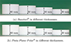 |
Figure 1 Four different thicknesses (30 mm, 40 mm, 50 mm, 60 mm) of the two materials Basotect ® and Pinta Plano Polar ®, samples with 100 mm diameter are shown. |
 |
Figure 2 Three different diameters (98 mm, 100 mm, 102 mm) of the two materials Basotect® and Pinta Plano Polar®, samples with 30 mm thickness are shown. |
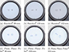 |
Figure 3 Specimens of different materials and different diameters mounted in the impedance tube. Edges are not sealed during the experiment. |
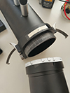 |
Figure 4 Angular rotation scale applied to the Brüel & Kjaer Type 4206 impedance tube. Only the 0°, 90°, 180°, and 270° marks are used for further investigations. |
The measurements are carried out in part during a master’s thesis [18]. For each combination of material, diameter, and thickness, three specimens are manufactured using the cutting device described in Section 3 to comply with the requirements of ISO 10534-2 [7]. Hence, 4 ⋅ 3 ⋅ 2 ⋅ 3 = 72 individual specimens are produced. Furthermore, considering the four mounting angles, a total of 96 combinations of factors are investigated. Each measurement setup is measured nine times, resulting in a total of 864 measurements conducted in randomised order. Randomisation of the measurements is performed based on the complete set to ensure unbiased results. The specimen installation within the tube can influence the diameter’s impact on the SAC. To enhance the repeatability of experiments, we install the specimen by applying uniform pressure, thereby preventing any deformations or indentations [19]. For the measurements, the impedance tube Brüel & Kjaer Type 4206 is used [15]. A sketch of the longitudinal cross-section of the impedance tube is depicted in Figure 5, for which the geometrical dimensions are specified in Table 1.
Geometric parameters of the Brüel & Kjaer Type 4206 impedance tube setup.
2 Measuring the sound absorption coefficient
The measurement of the sound absorption coefficient using the impedance tube with the two-microphone method is standardised in ISO 10534-2 [7]. This section provides an overview of the measurement method. In Figure 5, a sketch of the impedance tube setup is provided. To govern the measurement procedure, material measurements, data handling, and export, the Brüel & Kjaer PULSE LabShop software version 17.1.1 is used in conjunction with a Brüel & Kjaer Type 3560-B-130 signal conditioning unit.
As depicted in Figure 5, the impedance tube is driven by a loudspeaker, which plays back an excitation signal (i.e., Gaussian white noise) as generated by the signal generator. At the surface of the specimen, a partial reflection of the incident pressure wave occurs. Assuming plane wave propagation in the impedance tube, it is possible to describe the pressure field in the impedance tube by a superposition of incident and reflected wave such that
 (1)
(1)
where ℜ𝔢 denotes the real part,  and
and  denote the amplitudes of the incident and reflected part of the acoustic field, respectively. Furthermore,
  is the imaginary unit, ω = 2π
f is the angular frequency, and k = ω/c
0 is the wave number with
is the imaginary unit, ω = 2π
f is the angular frequency, and k = ω/c
0 is the wave number with  being the speed of sound in air computed from the bulk modulus Kair and density ρair of air at the ambient temperature. The microphones Mic. 1 and Mic. 2 shown in Figure 5 record time signals p1(t) and p2(t), respectively, which are transformed to the frequency domain, resulting in the complex-valued spectra
  and
and  defined as
 (2)
(2)
Thereby, x1 = d2 + d3 (see Fig. 5) and x2 = d3 are the positions of the two microphones Mic. 1 and Mic. 2, respectively. Furthermore, k0 is a complex wave number, for which the real and imaginary parts are computed with equations (A.1) and (A.2) of ISO 10534-2 [7], such that
 (3)
(3)
Herein, k
0′′ represents the attenuation due to the empty tube. Using the measured pressure spectra  and
and  and observing that
  , the transfer function H
12 between Mic. 1 and Mic. 2 can be obtained with
, the transfer function H
12 between Mic. 1 and Mic. 2 can be obtained with
 (4)
(4)
Preliminary measurements are necessary in order to compensate for phase and amplitude mismatches between Mic. 1 and Mic. 2, as defined in Annex A of ISO 10534-2 [7] and implemented in the governing software Brüel & Kjaer PULSE LabShop version 17.1.1. The preliminary measurements contain the following steps:
-
the channel calibration, i.e., the calibration of the microphones’ sound pressure level,
-
the measurement of the signal-to-noise ratio, and
-
the transfer function calibration.
During the last step of the preliminary measurements, H 12 is determined. Furthermore, measurements of ambient temperature, air pressure, and humidity are conducted in compliance with Annex A of ISO 10534-2 [7]. Following Annex C of ISO 10534-2 [7], the above relation can be rearranged for the reflection coefficient r such that
 (5)
(5)
After rearranging equation (2), the following transfer functions for the incident H i and reflected H r waves are used in equation (5), such that
 (6)
(6)
Finally, the sound absorption coefficient α can be computed from the reflection coefficient r using
 (7)
(7)
Note that α depends on frequency through the wave number k0.
2.1 Inverse computation of JCAL parameters by optimisation
In order to assess the parameters of the materials under investigation, it is assumed that the sound absorption properties of the material in question follow the Johnson–Champoux–Allard–Lafarge (JCAL) model [20–22]. The JCAL model is a semi-analytic absorption model for the effective density ρabs(ω) and the effective bulk modulus Kabs(ω) such that
![Mathematical equation: $$ \begin{aligned} \begin{split} \rho _\text{ abs}(\omega )&= \frac{\alpha _\infty \rho _\text{ air}}{\phi } \mathopen \mathclose {\left[ 1 + \frac{\sigma \phi }{\mathrm{j} \omega \rho _\text{ air} \alpha _\infty } \sqrt{1 + \mathrm{j} \frac{4 \alpha _\infty ^2 \eta _0 \rho _\text{ air} \omega }{\sigma ^2 \mathrm{\Lambda }^2 \phi ^2}} \right]},\\ K_\text{ abs}(\omega )&= \frac{\gamma p_0 / \phi }{\gamma - (\gamma -1)\mathopen \mathclose {\left[ 1 - \mathrm{j} \frac{\phi \kappa }{\bar{k}\prime _0 C_\mathrm{p} \rho _\text{ air} \omega } \sqrt{1 + \mathrm{j} \frac{4 \bar{k}\prime ^2_0 C_\mathrm{p} \rho _\text{ air} \omega }{\kappa \mathrm{\Lambda }\prime ^2 \phi ^2} } \right]}^{-1} }, \end{split} \end{aligned} $$](/articles/aacus/full_html/2025/01/aacus240145/aacus240145-eq17.gif) (8)
(8)
with the open porosity ϕ, the static airflow resistance σ, the high-frequency limit of the tortuosity α
∞, the viscous characteristic length Λ, the thermal characteristic length Λ′, and the static thermal permeability  . Note that both ρ
abs(ω) and K
abs(ω) are frequency-dependent and complex-valued. These are the frequency-independent six parameters of the JCAL model formulated in the parameter vector
. Note that both ρ
abs(ω) and K
abs(ω) are frequency-dependent and complex-valued. These are the frequency-independent six parameters of the JCAL model formulated in the parameter vector ![Mathematical equation: $ \vec{\theta}_{\mathrm{JCAL}} = [\phi \bar{k}_{0}\prime {\mathrm{\Lambda}} {\mathrm{\Lambda}}\prime \sigma \alpha_{\infty}]^{\mathrm{T}} $](/articles/aacus/full_html/2025/01/aacus240145/aacus240145-eq19.gif) . Furthermore, the constitutive parameters of air are the dynamic viscosity η
0, thermal conductivity κ, isentropic exponent γ, the ambient air pressure p
0, and the specific heat of air at constant ambient pressure C
p, for which the following values have been used, corresponding to the ambient conditions [4, Eq. (7)]:
. Furthermore, the constitutive parameters of air are the dynamic viscosity η
0, thermal conductivity κ, isentropic exponent γ, the ambient air pressure p
0, and the specific heat of air at constant ambient pressure C
p, for which the following values have been used, corresponding to the ambient conditions [4, Eq. (7)]:
 (9)
(9)
The characteristic impedance Z
JCAL(ω), the complex wave number k
JCAL in the porous material, and successively the reflection coefficient r
JCAL(ω) can be computed from ρ
abs(ω) and K
abs(ω) by assuming a two-port transmission model  , such that
![Mathematical equation: $$ \begin{aligned} \vec{T}_\mathrm{JCAL}&= \begin{bmatrix} T_{11}&\quad T_{12} \\[3pt] T_{21}&\quad T_{22} \end{bmatrix} \nonumber \\&= \begin{bmatrix} \cos \mathopen \mathclose {\left( k_\mathrm{JCAL} t \right)}&\quad \mathrm{j} Z_\mathrm{JCAL} \sin \mathopen \mathclose {\left( k_\mathrm{JCAL} t \right)} \\[3pt] \mathrm{j} \frac{1}{Z_\mathrm{JCAL} } \sin \mathopen \mathclose {\left( k_\mathrm{JCAL} t \right)}&\quad \cos \mathopen \mathclose {\left( k_\mathrm{JCAL} t \right)} \end{bmatrix}, \end{aligned} $$](/articles/aacus/full_html/2025/01/aacus240145/aacus240145-eq22.gif) (10)
(10)
where t denotes the thickness of the specimen and Z JCAL and k JCAL(ω) are the characteristic impedance and the complex wave number, respectively. They are related to the effective density and bulk modulus ρ JCAL and K abs, respectively, as follows
 (11)
(11)
From the two-port transmission line model in equation (10) follows the reflection coefficient
 (12)
(12)
where  is the characteristic impedance of air. Finally, using equation (7), the sound absorption coefficient α
JCAL(ω) is computed from r
JCAL(ω). This approach is also used in [4].
is the characteristic impedance of air. Finally, using equation (7), the sound absorption coefficient α
JCAL(ω) is computed from r
JCAL(ω). This approach is also used in [4].
To inversely determine the 6 parameters of the JCAL model  , an optimisation problem is set up according to [6, 23] as follows. The objective function to be minimised reads
 (13)
(13)
where α
ref(f) and  are the measured absorption coefficient and that calculated from the JCAL model, respectively, over the measurement frequency range from 150 Hz to 1600 Hz. A genetic algorithm minimises the L
2-norm of the difference of these absorption coefficients as described in [6, 23], where the same initial parameters as listed in [4], Tab. 2] are used. The result of the optimisation algorithm is an optimal set of JCAL parameters
are the measured absorption coefficient and that calculated from the JCAL model, respectively, over the measurement frequency range from 150 Hz to 1600 Hz. A genetic algorithm minimises the L
2-norm of the difference of these absorption coefficients as described in [6, 23], where the same initial parameters as listed in [4], Tab. 2] are used. The result of the optimisation algorithm is an optimal set of JCAL parameters  , which is used to compute the sound absorption coefficient
  . The reference sound absorption coefficient α
ref(f) is taken from the measurements with 0° angular rotation and averaged over the nine available measurements (three measurements for each of the three specimens).
. The reference sound absorption coefficient α
ref(f) is taken from the measurements with 0° angular rotation and averaged over the nine available measurements (three measurements for each of the three specimens).
Figure 6 compares the measured sound absorption coefficients αref(f) with the sound absorption coefficients obtained from the optimisation  for the two materials Basotect® and Pinta Plano Polar® in different diameters and thicknesses. The optimised JCAL parameters are listed in Appendix B. The JCAL model predicts the measured absorption coefficients well at 98 mm diameter over the entire frequency range for both materials. The prediction is acceptable for Basotect® with 100 mm and 102 mm diameter, but the local minima at 700–900 Hz and 500–700 Hz can not captured by the JCAL model. Pinta Plano Polar® (100 mm and 102 mm diameter) exhibits a similar drop of the absorption coefficient at 400 Hz, which does not depend on the diameter. It is assumed that the specimens are compressed to a certain extent when the diameter is 102 mm so that the edge constraints affect the measured absorption coefficients. This effect is not included in the JCAL model. However, it is yet unclear why the 100 mm specimens exhibit a similar behaviour. It may be the effect of a deviation from the real diameter of the specimen from the target diameter. Preliminary measurements of the real diameter of the specimens using a calliper show that the precision depends on the material, meaning that the diameter precision is better for Basotect® than for Pinta PlanoPolar®. A discussion on the diameter precision of the cutting device is provided in Section 3.4.
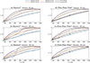 |
Figure 6 Comparison of the measured sound absorption coefficients and the result of the inverse fitting procedure using the JCAL model. |
3 Cutting device for specimen preparation
The accuracy of acoustic measurements can be compromised by specimens with non-nominal diameters or slightly irregular shapes, as highlighted in [10]. To mitigate this issue, a cutting device is developed, addressing the limitations inherent in the ISO 10534-2 [7], ASTM E1050-19 [8] and ASTM E2611-19 [9] standards. We propose a versatile tool for cutting specimens on a band saw. The workshop drawings of the cutting device are given as supplementary material to this article. The design of the cutting device is inspired by Stender et al.[13], Fig. 3b]. However, in [13], no publicly available CAD model or workshop drawings are available.
3.1 Requirements
The cutting device is designed to produce cylindrical specimens with high precision for measurements in an impedance tube. To ensure optimal performance and accuracy, the following design requirements R1–R4 are established for the cutting device:
-
R1 Dimensional accuracy: The device must ensure high diametrical precision, with tolerances within ±0.05 mm. This is essential to avoid shape deviations and ensure proper fit in the impedance tube, preventing measurement errors [10].
-
R2 Compatibility: The device is designed to work with a band saw. It must provide secure specimen clamping and effective vibration damping to maintain cutting accuracy during operation. The cutting device must hold the specimen firmly during the cutting procedure and, at the same time, not deform the material.
-
R3 Surface accuracy: The cutting process must result in clean edges and smooth surface finish in circumferential direction, minimising the need for smoothing the specimen surface after cutting, and ensuring the acoustic integrity of the specimens, i.e., not altering the acoustic properties of the specimens by compression or strain of the specimens.
-
R4 Versatility: The device must allow for cutting specimens of various diameters and thicknesses. This necessitates an easy and practical mechanism for adjusting components, ensuring quick setup and changeovers between different specimen sizes.
3.2 Design
The device consists of a base made of three aluminium plates, securely fastened together using conical screws (M8 × 40), ensuring a solid and rigid structure, see parts number 7–9 in Figure 7c. The cutting mechanism utilises two aluminium rods, each featuring two diameter reductions, connected to the base through two bushings that allow relative movement between the rods and the base. The bushing used in this study features an inner diameter of 20 mm, an outer diameter of 21 mm, and a bearing width of 20 mm. It is made from Iglidur G, a self-lubricating material [24]. The rods are depicted as parts number 6 and 11 in Figure 7c.
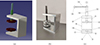 |
Figure 7 Views of the cutting device: (a) Three-dimensional view of the cutting device, generated from its computer-aided design (CAD) model in CATIA. (b) Photograph of the constructed cutting device, showing its detailed structure and components. Additional sandpaper is later applied to the inner surfaces of the plates to increase the friction between the specimen and the cutting device. Furthermore, a turning handle is later added to increase operational safety when cutting small diameters. (c) Sketched overview of the proposed cutting device. The complete set of workshop drawings is available as supplementary material. |
A steel height regulator (denoted as part number 12 in Fig. 7c), consisting of a hollow cylinder with a 4 mm threaded hole on the lateral surface, enables the precise adjustment of the cutting height, thus allowing the cutting of specimens with a thickness varying between 8 mm and 80 mm. This addresses the requirement R4.
Two aluminium plate supports, in the form of threaded hollow cylinders denoted as part number 3 in Figure 7c, are screwed into the first diameter reduction of the rods. Each support is connected to a plate of the desired specimen diameter, which is a hollow disk (without thread) and fits onto the rods’ second diameter reduction, see parts number 1 and 2 in 7c. The plates and therefore also the specimens may have diameters ranging from 26 mm to 260 mm, addressing the requirements R1 and R4. The plates are connected to the supports with three cylindrical screws (M3 × 10), which ensure a stable and precise mounting of the sample between the plates. Workshop drawings of all parts of the cutting device are provided as supplementary material.
To reduce friction and facilitate rotation, a lubricant (such as mineral oil or spray lubrication) has been applied to the rods. Furthermore, coarse-grained sandpaper is applied to the plates’ non-holed surfaces to increase the sliding friction between them and the specimen. This ensures that the latter does not slip during cutting and, therefore, addresses requirements R2 and R3.
3.3 Cutting procedure
To minimise uncertainty during the use of the cutting device, a step-by-step procedure protocol is proposed to ensure consistency and precision in the cutting process. The protocol steps are as follows:
-
Mounting the Plates: Attach the plates corresponding to the diameter of the specimen to thecutting device. This ensures that the specimen is properly aligned and supported throughout the cutting process.
-
Securing the Device: Rigidly fix the cutting device to the workbench on the bandsaw using clamps to prevent unintended movement during operation. Stability is key to achieving a precise cut. In Figure 8, an exemplary mounting situation with screw clamps is depicted at a bandsaw.
-
Adjusting the Plate Distance: Adjust the distance between the two plates based on the desired specimen thickness. This ensures that the specimen is securely clamped without causing deformation.
-
Material Incision: Perform an initial incision on the specimen material to allow proper alignment between the plates and the band saw blade. This step ensures that the circular specimen will have no straight edges and will result in cylindrical shape after cutting.
-
Cutting Execution: Carry out the cut by rotating the device via the height adjustment element. This controlled motion ensures a uniform cut around the entire circumference of the specimen. Make sure that the material does not slip during rotation or that the sand paper damages the specimens surface. Rotate the height adjustment element slowly and continuously.
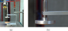 |
Figure 8 Placement of the cutting device with mounted plates for specimen with a diameter of t = 100 mm in close proximity to the band saw blade. (a) Cutting device secured on the workbench with a clamp. (b) Detail view of the upper plate with the band saw blade. |
A video of the usage of the cutting device is provided in the supplementary material of this publication to demonstrate the actual use of the cutting device on a bandsaw.
3.4 Precision of the produced specimens
The precision of the specimens produced with the cutting device is analysed by measuring the diameter of the specimens with a calliper at four cross-sections of each specimen (at 0° and 90° at the top and bottom surfaces of the specimens). The four cross-sectional measurements are averaged to achieve a representative diameter for each specimen. The diameter measurements are part of the FOAM 02-dataset, as described in Appendix A. A box plot of the diameter measurement result is depicted in Figure 9. While it seems from Figure 9 that Basotect® can be cut with a higher precision overall than Pinta Plano Polar®, the following should be considered: The calliper applies a measurement force to the specimen that slightly deforms it. The melamine foam is softer than the PET fiber plate, thus, it is more compliant with deformations caused by the calliper measurement force. Even with these deviations, the diameter precision of the specimens produced with the cutting device is wellbelow 1 mm.
 |
Figure 9 Measurements of the specimen’s diameters using a calliper. |
4 Results
A preliminary study is proposed to observe the data distribution in the frequency domain. Violin plot analysis provides a visual representation of a dataset’s distribution. The analysis of the violin plots is performed by scalarising the sound absorption coefficient. A representative scalar SAC value α scalar is obtained by taking the median of the frequency-dependent SAC. The violin plots in Figure 10 show the distribution of αscalar across one factors at different materials. Figure 10a depicts the distribution of αscalar for different thicknesses. Clearly, the specimen thickness has a distinct effect on the median SAC αscalar. Figure 10b depicts the distribution of αscalar for different diameters. From this perspective, specimens with different thicknesses are grouped together, resulting in a multivariate distribution for the three diameters. Figure 10c shows the distribution of αscalar for the four rotational angles. The distribution of αscalar exhibits four local maxima, similar to Figure 10b. However, it appears that the factors diameter and rotational angle have different effects on the distribution of αscalar, because of the differently shaped distributions.
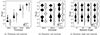 |
Figure 10 Violin plot of α scalar regarding combinations between factors. |
The same pre-processing algorithm as in [13] is applied also for the measurement data in this study. This enables a cross-compatibility and direct comparison of the datasets FOAM 01 [25] and FOAM 02 [26].
In Figures 11 and 12, the mean μ and standard deviation σ of the SAC α is depicted as a function of frequency for the two investigated materials (Pinta Plano Polar® and Basotect®). The graphs in Figures 11 and 12 demonstrate the variability in acoustic performance across different frequency ranges for bothmaterials.
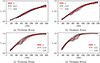 |
Figure 11 108 SAC measurements α n (f) per thickness, with mean μ and standard deviation σ for the PET fiber plate (Pinta Plano Polar ®). |
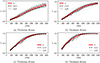 |
Figure 12 108 SAC measurements α n (f) per thickness, with mean μ and standard deviation σ for the melamine resin foam (Basotect ®). |
5 Discussion and conclusion
In this publication, the creation of the FOAM 02 dataset containing 864 measurements of the sound absorption coefficient of Basotect® and Pinta PlanoPolar® is documented, following previous work [13, 25]. Four factors have been considered during the creation of the dataset: diameter inaccuracies, specimen thickness, angular rotation of the specimen, and different materials. The dataset is publicly available in the benchmark dataset collection of the European Acoustics Association [26]. It contains the measured sound absorption coefficients, the one-hot encoded label vectors, and a detailed documentation for further usage.
One challenge when preparing specimens for impedance tube measurements is the cutting procedure [11]. Previous research suggests that air-gaps affect the sound absorption coefficient [10] due to specimens that are slightly smaller than the nominal diameter of the impedance tube. Slightly larger diameters squeeze the specimens at the edges and affect the measurements as well. In addition, shape deviations may further introduce uncertainty. For an uncertainty analysis of the measurement procedure, a calibrated reference material would be necessary. Previous reproducibility experiments highlight that the reproducibility of impedance tube measurements can be improved, particularly by using a standardised procedure for material preparation [11]. Thus, it is necessary to cut the specimens very accurately. In Section 3, the design of a cutting device for use with a band-saw is proposed with the aim of facilitating the accurate cutting of specimens. The workshop drawings of the cutting device are available as supplementary material to this paper. The cutting device could help to reduce measurement uncertainties that govern from inaccurately cut specimens.
The outcome of this paper is twofold: First, our FOAM 02 dataset is provided to the scientific community for machine learning purposes. The FOAM 02 dataset is compatible with the FOAM 01 dataset so that both datasets can be used for transfer learning approaches. Second, a procedure to precisely cut specimens of porous materials on a bandsaw is provided, including a detailed design of a cutting device. This device reduces uncertainty in both diameter and shape of the specimen. Currently, the device has only been tested with 2 materials, and its general applicability to other materials, like fibrous materials, requires further testing.
Acknowledgments
The authors thank Daniel Eisenkölbl, Tim Reisenhofer, and Angelique-Marie Handl from the Institute of Electronics (IFE) at Graz University of Technology for manufacturing the cutting device according to the drawings developed by the authors. The authors thank Gerald Maurer from IGTE for making the photographs shown in Figures 1, 2, 3, and 8, as well as the video provided as supplementary material. The authors thank Patricia Grabowska for performing the diameter measurements presented in Table A.3.
Funding
F. K., C. A., and M. K. received funding from the “BMIMI Endowed Professorship on Noise Impact Research: Competence Center for Traffic Noise and Health" of the Austrian Research Promotion Agency (FFG) under project No. FO999891611. A. W. and S. S. received funding from the COMET project ECHODA (“Energy Efficient Cooling and Heating of Domestic Appliances”) under FFG project No. FO999913905. ECHODA is funded within the framework of “COMET – Competence Centers for Excellent Technologies" by BMIMI, BMAW, the province of Styria, and SFG. The COMET program is managed by FFG. J. B. and S. S. received funding from the FFG under project No. FO999913972. Supported by TU Graz Open Access Publishing Fund.
Conflicts of interest
The authors declare that they have no conflicts of interest in relation to this article.
Data availability statement
The dataset containing (i) the one-hot encoded target vectors, (ii) the sound absorption coefficient over frequency, and (iii) the diameter measurements of the specimens using a calliper is available in Zenodo, under the reference [26]. A description of the dataset is provided in Appendix A.
Supplementary material
suppl1.pdf: The complete set of workshop drawings of the proposed cutting device in PDF format. Access Supplementary Material
suppl2.mp4: A short video demonstrating the use of the proposed cutting device in MP4 format. Access Supplementary Material
References
- K.V. Horoshenkov: A review of acoustical methods for porous material characterisation. The International Journal of Acoustics and Vibration 22, 1 (2017) 92–103. [Google Scholar]
- N. Hiremath, V. Kumar, N. Motahari, D. Shukla: An overview of acoustic impedance measurement techniques and future prospects. Metrology 1, 1 (2021) 17–38. [Google Scholar]
- A. Pereira, A. Gaspar, L. Godinho, P. Amado Mendes, D. Mateus, J. Carbajo, J. Ramis, P. Poveda: On the use of perforated sound absorption systems for variable acoustics room design. Buildings 11, 11 (2021) 543. [Google Scholar]
- F. Kraxberger, E. Kurz, W. Weselak, G. Kubin, M. Kaltenbacher, S. Schoder: A validated finite element model for room acoustic treatments with edge absorbers. Acta Acustica 7 (2023) 48. [Google Scholar]
- M. Vorländer: Computer simulations in room acoustics: concepts and uncertainties. The Journal of the Acoustical Society of America 133, 3 (2013) 1203–1213. [CrossRef] [PubMed] [Google Scholar]
- S. Floss, F. Czwielong, M. Kaltenbacher, S. Becker: Design of an in-duct micro-perforated panel absorber for axial fan noise attenuation. Acta Acustica 5 (2021) 24. [CrossRef] [EDP Sciences] [Google Scholar]
- International Organization for Standardization: ISO 10534-2:2023(E) Acoustics – Determination of sound absorption coefficient and impedance in impedance tubes – Part 2: Two-microphone technique for normal sound absorption coefficient and normal surface impedance, 2023. [Google Scholar]
- E33 Committee: ASTM E1050-19 test method for impedance and absorption of acoustical materials using a tube, two microphones and a digital frequency analysis system, 2019.DOI: https://doi.org/10.1520/E1050-19. [Google Scholar]
- E33 Committee: ASTM E2611-19 test method for normal incidence determination of porous material acoustical properties based on the transfer matrix method, 2019.DOI: https://doi.org/10.1520/E2611-19. [Google Scholar]
- A. Cummings: Impedance tube measurements on porous media: the effects of air-gaps around the sample. Journal of Sound and Vibration 151, 1 (1991) 63–75. [CrossRef] [Google Scholar]
- K.V. Horoshenkov, A. Khan, F.-X. Bécot, L. Jaouen, F. Sgard, A. Renault, N. Amirouche, F. Pompoli, N. Prodi, P. Bonfiglio, G. Pispola, F. Asdrubali, J. Hübelt, N. Atalla, C.K. Amédin, W. Lauriks, L. Boeckx: Reproducibility experiments on measuring acoustical properties of rigid-frame porous media (round-robin tests). The Journal of the Acoustical Society of America 122, 1 (2007) 345–353. [Google Scholar]
- T. Schultz, M. Sheplak, L.N. Cattafesta: Uncertainty analysis of the two-microphone method. Journal of Sound and Vibration 304, 1, 2 (2007) 91–109. [Google Scholar]
- M. Stender, C. Adams, M. Wedler, A. Grebel, N. Hoffmann: Explainable machine learning determines effects on the sound absorption coefficient measured in the impedance tube. The Journal of the Acoustical Society of America 149, 3 (2021) 1932–1945. [Google Scholar]
- M. Stender, M. Wedler, N. Hoffmann, C. Adams: Explainable machine learning: a case study on impedance tube measurements, in: Inter-Noise – 50th International Congress and Exposition on Noise Control Engineering. Washington, DC, USA, August 2021, pp. 3223–3234. [Google Scholar]
- Brüel & Kjaer: Impedance tube kit type 4206. www.bksv.com/media/doc/Bp1039.pdf, Last access on2024-12-09. [Google Scholar]
- BASF: Basotect – The versatile melamine resin foam. https://www.construction.basf.us/files/pdf/Basotect_brochure.pdf, Last access on 2024-12-09. [Google Scholar]
- Pinta Acoustic GmbH: Pinta Plano Polar. https://www.pinta-acoustic.de/cms/upload/Download-PDFs/Verklebesysteme/Technische_Merkblaetter/TM_Plano_Polar_2004.pdf, Last access on 2024-12-09. [Google Scholar]
- A. Caiazzo: Explainable machine learning determines potential uncertainty factors related to tube impedance measurements of the sound absorption coefficient. Master’s thesis, Universita Federico II, Naples, IT, 2024. [Google Scholar]
- H. Koruk: An assessment of the performance of impedance tube method. Noise Control Engineering Journal 62, 4 (2014) 264–274. [Google Scholar]
- D.L. Johnson, J. Koplik, R. Dashen: Theory of dynamic permeability and tortuosity in fluid-saturated porous media. Journal of Fluid Mechanics 176 (1987) 379–402. [Google Scholar]
- Y. Champoux, J.-F. Allard: Dynamic tortuosity and bulk modulus in air-saturated porous media. Journal of Applied Physics 70, 4 (1991) 1975–1979. [CrossRef] [Google Scholar]
- D. Lafarge, P. Lemarinier, J.F. Allard, V. Tarnow: Dynamic compressibility of air in porous structures at audible frequencies. The Journal of the Acoustical Society of America 102, 4 (1997) 1995–2006. [CrossRef] [Google Scholar]
- S. Floss: Mitigation of sound by micro-perforated absorbers in different types of sound fields – design and evaluation. PhD thesis, TU Wien, 2022. [Google Scholar]
- Igus: Iglidur G Sleeve Bearing. https://www.igus.eu/iglidur-ibh/sleeve-bearings/product-details/iglidur-g-m, Last access on 2024-12-09. [Google Scholar]
- C. Adams, A. Grebel, S. Wenzel, S. Schoder, M. Kaltenbacher: FOAM 01: Acoustic Material, https://doi.org/10.5281/ZENODO.10551343, January 2024x. [Google Scholar]
- A. Caiazzo, F. Kraxberger, C. Adams, A. Wurzinger, G. Petrone, S. Schoder, S. De Rosa, M. Kaltenbacher: FOAM 02: Impedance tube measurements of two porous materials with diameter variation, https://doi.org/10.5281/zenodo.14190550, 2024. [Google Scholar]
Appendix A Description of the FOAM 02 dataset
The dataset consists of three .csv-files: – The file targets.csv contains the one-hot encoded feature set of each measurement, meaning that each applicable factor gets assigned the value 1, whereas all false factors have the value 0. An excerpt of the file targets.csv is listed in Table A.1. The investigated factors are described in Section 1.1. As three specimen have been produced for each factor combination, also the specimen number is listed in Table A.1. Furthermore, each specimen is measured repeatedly three times, therefore also the repetition number is included in Table A.1. As discussed in Section 1.1, the measurements have been carried out in random order, such that potential systematic errors are evenly distributed across the dataset.
– The file alphas.csv contains the measured sound absorption coefficient over frequency f, such that each row contains one measurement. An excerpt of the file alphas.csv is listed in Table A.2. The evaluation frequencies range from 150 Hz to 1500 Hz in a 2 Hz-interval.
– The file diameters.csv contains the diameter measurements of the specimens produced with the proposed cutting tool. A calliper is used for the diameter measurements, as described in Section 3.4. In total, 72 individual specimens were produced (each was measured for four rotational angles and three repetitions, resulting in 864 SAC measurements). To be consistent with the other files in the FOAM 02-dataset, the file diameters.csv also has 864 rows, and the diameter measurement results are copied for identical specimens. An excerpt of the file diameters.csv is listed in Table A.3.
The measurement results stored in alphas.csv and diameters.csv can be related to the corresponding features stored in targets.csv via the measurement number.
Appendix B Results of inverse computation of JCAL parameters by optimisation
In Table B1, the optimal parameters of the JCAL model are shown for the material Basotect® with a rotation of 0° in different diameters and thicknesses. Table B.2 shows the optimal parameters of the JCAL model for the material Pinta Plano Polar® with a rotation of 0° in different diameters and thicknesses. As described in Section 2.1, the JCAL parameters listed in Table B.1 can be used to obtain the fitted sound absorption coefficients depicted in Figures 6a–6c, and the parameter values listed in Table B.2 correspond to Figures 6d–6f.
Extract of targets.csv.
Extract of alphas.csv.
Extract of diameters.csv.
Inversely determined parameters of the JCAL model for Basotect® with a rotation of 0°.
Inversely determined parameters of the JCAL model for Pinta Plano Polar ® with a rotation of 0°.
Cite this article as: Caiazzo A. Kraxberger F. Wurzinger A. Boysen J. Petrone G. Schoder S. De Rosa S. Kaltenbacher M. & Adams C. 2025. FOAM 02: A dataset of impedance tube measurements with different materials and diameter variations. Acta Acustica, 9, 50. https://doi.org/10.1051/aacus/2025033.
All Tables
Inversely determined parameters of the JCAL model for Basotect® with a rotation of 0°.
Inversely determined parameters of the JCAL model for Pinta Plano Polar ® with a rotation of 0°.
All Figures
|
Figure 1 Four different thicknesses (30 mm, 40 mm, 50 mm, 60 mm) of the two materials Basotect ® and Pinta Plano Polar ®, samples with 100 mm diameter are shown. |
| In the text | |
|
Figure 2 Three different diameters (98 mm, 100 mm, 102 mm) of the two materials Basotect® and Pinta Plano Polar®, samples with 30 mm thickness are shown. |
| In the text | |
|
Figure 3 Specimens of different materials and different diameters mounted in the impedance tube. Edges are not sealed during the experiment. |
| In the text | |
|
Figure 4 Angular rotation scale applied to the Brüel & Kjaer Type 4206 impedance tube. Only the 0°, 90°, 180°, and 270° marks are used for further investigations. |
| In the text | |
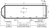 |
Figure 5 Sketch of the impedance tube setup using two microphones as specified in ISO 10534-2 [7]. |
| In the text | |
|
Figure 6 Comparison of the measured sound absorption coefficients and the result of the inverse fitting procedure using the JCAL model. |
| In the text | |
|
Figure 7 Views of the cutting device: (a) Three-dimensional view of the cutting device, generated from its computer-aided design (CAD) model in CATIA. (b) Photograph of the constructed cutting device, showing its detailed structure and components. Additional sandpaper is later applied to the inner surfaces of the plates to increase the friction between the specimen and the cutting device. Furthermore, a turning handle is later added to increase operational safety when cutting small diameters. (c) Sketched overview of the proposed cutting device. The complete set of workshop drawings is available as supplementary material. |
| In the text | |
|
Figure 8 Placement of the cutting device with mounted plates for specimen with a diameter of t = 100 mm in close proximity to the band saw blade. (a) Cutting device secured on the workbench with a clamp. (b) Detail view of the upper plate with the band saw blade. |
| In the text | |
|
Figure 9 Measurements of the specimen’s diameters using a calliper. |
| In the text | |
|
Figure 10 Violin plot of α scalar regarding combinations between factors. |
| In the text | |
|
Figure 11 108 SAC measurements α n (f) per thickness, with mean μ and standard deviation σ for the PET fiber plate (Pinta Plano Polar ®). |
| In the text | |
|
Figure 12 108 SAC measurements α n (f) per thickness, with mean μ and standard deviation σ for the melamine resin foam (Basotect ®). |
| In the text | |
Current usage metrics show cumulative count of Article Views (full-text article views including HTML views, PDF and ePub downloads, according to the available data) and Abstracts Views on Vision4Press platform.
Data correspond to usage on the plateform after 2015. The current usage metrics is available 48-96 hours after online publication and is updated daily on week days.
Initial download of the metrics may take a while.