| Issue |
Acta Acust.
Volume 10, 2026
|
|
|---|---|---|
| Article Number | 27 | |
| Number of page(s) | 4 | |
| Section | Ultrasonics | |
| DOI | https://doi.org/10.1051/aacus/2026028 | |
| Published online | 09 April 2026 | |
Short Communication
On the influence of the stress gradient on propagation behaviour of Rayleigh waves
1
Materials Center Leoben Forschung GmbH, Vordernbergerstraße 12, 8700 Leoben, Austria
2
Chair of Mechanics, Montanuniversität Leoben, Franz-Josef Straße 18, 8700 Leoben, Austria
* Corresponding author: This email address is being protected from spambots. You need JavaScript enabled to view it.
Received:
13
October
2025
Accepted:
13
March
2026
Abstract
This short communication presents a new combined numerical and signal processing based analysis of the influence of stress gradients on Rayleigh wave propagation. The method uses finite element simulations based on the hyperelastic Murnaghan model, to caputure the acoustoelastic effect, and an adapted coda Wave Interferometry (CWI) technique to quantify time shift and stretch of Rayleigh wave signals. It is shown that the stress gradient alters both wave velocity and wave shape. While tensile stress reduces wave velocity, a stress gradient can counteract this effect and even enhance the propagation velocity. The combined evaluation of time shift and stretch allows an effective description of the influence of both surface stress and stress gradient on the wave propagation.
Key words: Rayleigh wave / Coda wave interferometry (CWI) / Finite element analysis
© The Author(s), Published by EDP Sciences, 2026
 This is an Open Access article distributed under the terms of the Creative Commons Attribution License (https://creativecommons.org/licenses/by/4.0), which permits unrestricted use, distribution, and reproduction in any medium, provided the original work is properly cited.
1 Introduction
Rayleigh waves are well suited for near-surface residual stress assessment because their effective penetration depth scales with wavelength and can thus be tuned by the excitation frequency. The observed stress dependence of propagation velocity originates from the acoustoelastic effect, which requires a nonlinear constitutive description (e.g., the Murnaghan model) rather than linear elasticity [1–5]. Since Crecraft’s pioneering work [6], ultrasonics can be used for (residual) stress detection, often with body-wave configurations such as LCR waves in welded or cast components [7, 8]. However, real engineering parts typically exhibit stress gradients. These gradients induce a depth-dependent wave velocity and, consequently, waveform distortion (dispersion), which can bias classical time-of-flight (ToF) evaluations that rely on velocity shift alone [9–12].
This short communication addresses the questions of how and how strongly stress gradients influence Rayleigh wave propagation, and how this influence can be robustly separated from the influence of the stress. Our approach combines (i) a numerical study using the isotropic hyperelastic Murnaghan model in ABAQUS/Explicit to systematically vary surface stress and gradient, with (ii) an adapted coda-wave interferometry (CWI) procedure applied directly to the measured Rayleigh wave [13, 14]. The method extracts two independent observables from a single surface trace: shift (time delay ⇒ velocity change) and stretch (temporal dilation ⇒ gradient-induced dispersion). The numerical results indicate that increasing tensile stress reduces Rayleigh wave velocity, whereas increasing stress gradient raises the apparent velocity because the average stress within the penetration depth decreases. Gradients produce measurable dispersion, particularly at lower frequencies where the penetration depth is larger. We condense these trends into compact regression relations, introducing the concept of effective measured stress.
2 M aterials and methods
2.1 Material model and FE setup
Rayleigh wave propagation is simulated in ABAQUS/Explicit using the isotropic, weakly nonlinear hyperelastic Murnaghan model implemented via a Fortran VUMAT subroutine. Second-order (Lamé) constants are λ = 90 900 MPa and μ = 78 000 MPa; third-order (Murnaghan) constants are ν 1 = 358 000 MPa, ν 2 = −265 000 MPa, ν 3 = −182 000 MPa. The elastic potential U for the Murnaghan model as function of the Green–Lagrange strain tensor E is given by:
 (1)
(1)
The domain is a cuboid solid meshed with C3D8R elements; to resolve the wavefield, the element edge length is set to a = λ RW/10, where λ RW denotes the wave length of the Rayleigh wave. Different stress fields are introduced in a preceding quasi-static step as a depth-dependent normal stress σ(y) defined by an analytical field; the subsequent dynamic step simulates wave excitation and reception. A surface pressure p(t) over a small patch excites the Rayleigh wave with time history (burst). Two virtual surface sensors on the FE model, separated by Δx = 100 mm, record out-of-plane particle velocity with a sampling rate ≥20 f. The numerical model is shown in Figure 1.
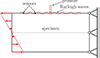 |
Figure 1. Sketch of the numerical model with the load, support, wave initiation and virtual sensors for detecting the elastic wave. |
2.2 Stress states and gradients
We study surface stresses σ 1 and linear depth gradients dσ/dy within |σ 1|≤600 MPa and |dσ/dy|≤60 MPa/mm. Figure 2 shows the investigated stress distributions. For characterisation of the different stress distributions, Siebel’s normalised stress gradient χ [15] is used.
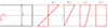 |
Figure 2. Variation of the stress gradient. (a) Pure bending stress (χ = 2/h), (b) Bending stress superimposed with tensile stress (χ = 1/h), (c) Bending stress superimposed with tensile stress (χ = 1/(2h)), (d) Pure tensile stress (χ = 0). |
 (2)
(2)
2.3 Adapted coda-wave interferometry (CWI)
To robustly extract small velocity changes and gradient-induced waveform distortions, an adapted CWI is applied directly to the recorded Rayleigh wave signal. After band-pass filtering around f, the relevant portion of the waveform is divided into short windows [t 1, t 2], and for each window the normalised cross-correlation (Eq. (4)) is evaluated.
 (3)
(3)
A two-step procedure is used: (i) estimate a global stretch factor Λ by maximising the correlation over scaled time axes; de-stretch u stress accordingly; (ii) compute the residual fixed shift Δt by maximising R over pure time shifts. Both quantities are averaged over the burst support windows.
The optimal time shift t s that maximises the correlation is plotted against the window centre t c , and the local velocity change follows Δv/v = −t s */t c . The stretch factor is obtained from the slope of this relation. In our implementation, a global stretch is first determined by maximising equation (4) over scaled time axes and u stress is de-stretched accordingly. A second CWI pass on the de-stretched signal then yields the residual fixed shift. This two-step procedure provides a robust and unique pair of observables–stretch and shift–from a single Rayleigh trace.
3 Results
Shift and stretch are governed by both surface stress and stress gradient. Applying the adapted CWI directly to the Rayleigh wave signal provides two observables from a single trace. Figure 3 isolates the effect of the normalised gradient χ at fixed surface stress σ1. The shift Δt decreases as tensile stress increases (reduced velocity) and increases under compression (increased velocity). For a given σ1, a larger χ systematically reduces the absolute shift, i.e., gradients bias the ToF toward smaller total time shifts |Δt|.
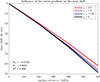 |
Figure 3. Influence of different normalised stress gradients on the total shift for same surface stresses. |
The time shift Δt is observed to follow
 (4)
(4)
K 0 represents the acoustoelastic constant and thus quantifies the sensitivity of the wave velocity to a homogeneous stress state. K 1 accounts for the additional influence of the normalised stress gradient. K 1 can be regarded as a gradient-dependent acoustoelastic constant where K 0 is the acoustoelastic constant and K 1 is a corrective term for the influence of the stress gradient, with R 2 ≈ 0.996. This confirms that gradients systematically reduce the absolute time shift for a given surface stress. We define the effective measured stress as the stress of a hypothetical gradient-free (uniform) state that results in the same total shift as the true stress state. If the stress distribution is known, the effective stress depth follows from
 (5)
(5)
where t
eff is the depth where the effective measured stress acts. It can be shown that  . Figure 4 plots the stretch Λ as a function of the effective stress σeff for several normalised stress gradients χ. For a homogeneous profile (χ = 0), Λ attains its minimum, whereas the largest gradient yields the maximum Λ. Overall, at fixed σeff the stretch increases monotonically with χ, consistent with gradient-induced dispersion of the Rayleigh wave.
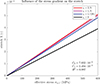 |
Figure 4. Influence of different stress distributions on the resulting stretch of elastic surface waves as a function of the effective stress. |
The stretch Λ, which quantifies waveform distortion due to depth-varying velocity, is well described by
 (6)
(6)
with R 2 ≈ 0.987. C 0 and C 1 are model constants. Coefficients K 0, K 1, C 0, C 1 are obtained by regression from FE datasets.
4 Discussion
Our simulations clarify how stress and, in particular, its depth gradient govern Rayleigh wave propagation. Two robust trends emerge and are internally consistent across all cases studied: (i) increasing tensile stress reduces the Rayleigh velocity (negative shift), and (ii) a positive gradient increases the apparent velocity, which manifests as a smaller absolute time shift for the same surface stress (Fig. 3). In parallel, the waveform distortion captured by the stretch grows with the normalised gradient χ at fixed effective stress (Fig. 4). Together, these observations explain why classical time-of-flight (ToF) evaluations that ignore gradients can bias near-surface residual-stress estimates. The results further indicate that the classical TOF method measures the effective stress–rather than the surface or the average stress within the propagation depth.
The gradient effect can be interpreted as a depth-weighting phenomenon: the measured signal integrates a stress-dependent velocity over the sampling region so that a tensile surface stress combined with a positive gradient yields a lower depth-averaged stress and, hence, a higher apparent velocity. This is captured by the compact regressions used here, where the gradient contribution gains weight as frequency decreases. Conversely, the influence of a homogeneous stress state on the observed timing over the MHz band is small compared to the gradient-driven effect seen in Λ.
Using the adapted CWI, we extract two trace-level observables that respond differently to the stress field: the shift follows Δt = (K 0 + K 1 χ)σ 1 and the stretch follows Λ = (C 0 + C 1 χ)σ eff with σ eff = Δt/K 0. This pairing resolves the identifiability problem inherent to shift-only methods: combining Δt and Λ in a minimal inversion allows separation of surface stress and gradient and yields a concise, frequency-aware reconstruction workflow suitable for short-measurement campaigns.
Our simulations reveal that the penetration depth of Rayleigh waves is inherently frequency-dependent. Two consistent findings emerge: (i) the model parameters K2 and C2 vary systematically with excitation frequency, and (ii) this frequency dependence governs the apparent propagation velocity through the effective penetration depth. Together, these insights explain why analyses assuming constant K2 and C2 may lead to biased inversions. Consequently, solving the inverse problem requires an explicit determination of the frequency-dependent behaviour of K2(f) and C2(f).
The study assumes isotropy and a weakly nonlinear Murnaghan law; prior plastic deformation and anisotropy are represented only via effective constants. Linear stress profiles are considered; higher-order gradients and microstructural heterogeneity are not resolved. Numerical dispersion and finite-domain effects were mitigated but cannot be fully excluded. Future work will calibrate the coefficients on well-characterised specimens, extend the framework to anisotropic or textured materials, and validate the two-observable inversion on experimental data across multiple frequencies and representative stress profiles.
5 Conclusion
This short communication numerically quantified how stress gradients govern Rayleigh wave propagation and showed how an adapted coda-wave interferometry can extract two complementary observables–shift and stretch–from a single surface trace. Based on FE simulation using Murnaghans hyperelastic material model, we found that tensile stress decreases, while stress gradients increase the apparent Rayleigh velocity; gradients also induce measurable dispersion. Compact regressions link shift and stretch to surface/effective stress and gradient, enabling a straightforward inversion that introduces the practical notions of effective measured stress and stress gradient. This approach provides a concise route to separate stress from gradient and to reconstruct near-surface residual-stress profiles. Future work should focus on experimental calibration (temperature/roughness), anisotropy and microstructural effects, and multi-frequency validation on reference specimens.
Acknowledgments
The authors thank the Austrian Research Promotion Agency (FFG) for financial support in project FO999899048.
Funding
The research was funded by the Austrian Research Promotion Agency (FFG) in project FO999899048.
Conflicts of interest
The authors declare no conflict of interest.
Data availability statement
The data is available on request by the authors.
Author contribution statement
Conceptualization (Marcel Ruetz), Data curation (Marcel Ruetz), Formal analysis (Marcel Ruetz), Funding acquisition (Hans-Peter Gänser), Investigation (Marcel Ruetz), Methodology (Marcel Ruetz), Project administration (Hans-Peter Gänser), Resources (Hans-Peter Gänser), Software (Marcel Ruetz), Supervision (Thomas Antretter & Hans-Peter Gänser), Validation (Marcel Ruetz), Visualization (Marcel Ruetz), Writing – original draft (Marcel Ruetz), Writing – review & editing (Marcel Ruetz & Thomas Antretter & Hans-Peter Gänser).
References
- F.D. Murnaghan: Finite deformations of an elastic solid. American Journal of Mathematics 59 (1937) 235–260. [Google Scholar]
- D.S. Hughes, J.L. Kelly: Second-order elastic deformation of solids. Physical Review 92 (1953) 1145–1149. [Google Scholar]
- M. Hayes, R.S. Rivlin: Propagation of a plane wave in an isotropic elastic material subjected to pure homogeneous deformation. Archive for Rational Mechanics and Analysis 8 (1961) 15–22. [Google Scholar]
- R.A. Toupin, B. Bernstein: Sound waves in deformed perfectly elastic materials. Acoustoelastic effect. Journal of the Acoustical Society of America 33 (1961) 216–225. [Google Scholar]
- M. Ruetz, T. Antretter, H.-P. Gänser: Numerical investigation of the influence of the stress multiaxiality on the propagation behavior of Rayleigh waves. Applied Sciences 15, 16 (2025) 9109. [Google Scholar]
- D.I. Crecraft: The measurement of applied and residual stresses in metals using ultrasonic waves. Journal of Sound and Vibration 5 (1967) 173–192. [Google Scholar]
- T. Leon-Salamanca: Ultrasonic measurement of residual stress in steels using critically refracted longitudinal waves (LCR), Texas A & M University, Department of Mechanical Engineering, 1988. [Google Scholar]
- M. Srinivasan, D.E. Bray, P. Junghans, A. Alagarsamy: Critically Refracted Longitudinal Waves Technique: a New Tool for the Measurement of Residual Stresses in Castings. Vol. 99. AFS (American Foundrymen Society), 1991. [Google Scholar]
- C. Bescond, J.-P. Monchalin, D. Levesque, A. Gilbert, R. Talbot: Determination of residual stresses using laser-generated surface skimming longitudinal waves, in: Nondestructive Evaluation and Health Monitoring of Aerospace Materials, Composites, and Civil Infrastructure IV. Proceedings of the SPIE. Vol. 5767, 2005. doi: https://doi.org/10.1117/12.620374. [Google Scholar]
- M.O. Si-Chaib, S. Menad, H. Djelouah, M. Bocquet: An ultrasound method for the acoustoelastic evaluation of simple bending stresses. NDT & E International 34 (2001) 521–529. [Google Scholar]
- M.O. Si-Chaib, H. Djelouah, T. Boutkedjrt: Propagation of ultrasonic waves in materials under bending forces. NDT & E International 38 (2005) 283–289. [Google Scholar]
- Y. Ivanova, T. Partalin: Investigation of stress-state in rolled sheets by ultrasonic techniques. Ultrasound 66, 1 (2011) 7–15. [Google Scholar]
- R. Snieder: The theory of coda wave interferometry. Pure and Applied Geophysics 163, 2–3 (2006) 455–473. [Google Scholar]
- R. Snieder, A. Gret, H. Douma, J. Scales: Coda wave interferometry for estimating nonlinear behavior in seismic velocity. Science 295, 5563 (2002) 2253–2255. [Google Scholar]
- E. Siebel, M. Stieler: Dissimilar stress distributions and cyclic loading. Zeitschrift des Vereines Deutscher Ingenieure 97 (1955) 121–131. [Google Scholar]
Cite this article as: Ruetz M. Antretter T. & Gänser H.-P. 2026. On the inuence of the stress gradient on propagation behaviour of Rayleigh waves. Acta Acustica, 10, 27. https://doi.org/10.1051/aacus/2026028.
All Figures
|
Figure 1. Sketch of the numerical model with the load, support, wave initiation and virtual sensors for detecting the elastic wave. |
| In the text | |
|
Figure 2. Variation of the stress gradient. (a) Pure bending stress (χ = 2/h), (b) Bending stress superimposed with tensile stress (χ = 1/h), (c) Bending stress superimposed with tensile stress (χ = 1/(2h)), (d) Pure tensile stress (χ = 0). |
| In the text | |
|
Figure 3. Influence of different normalised stress gradients on the total shift for same surface stresses. |
| In the text | |
|
Figure 4. Influence of different stress distributions on the resulting stretch of elastic surface waves as a function of the effective stress. |
| In the text | |
Current usage metrics show cumulative count of Article Views (full-text article views including HTML views, PDF and ePub downloads, according to the available data) and Abstracts Views on Vision4Press platform.
Data correspond to usage on the plateform after 2015. The current usage metrics is available 48-96 hours after online publication and is updated daily on week days.
Initial download of the metrics may take a while.