


| Issue |
Acta Acust.
Volume 10, 2026
|
|
|---|---|---|
| Article Number | 54 | |
| Number of page(s) | 11 | |
| Section | Musical Acoustics | |
| DOI | https://doi.org/10.1051/aacus/2026041 | |
| Published online | 07 July 2026 | |
Technical & Applied Article
Designing a speckle interferometer for violin acoustics
Laboratorio de Acústica, Escuela de Laudería, Instituto Nacional de Bellas Artes y Literatura, Hidalgo #20 Centro, Querétaro Qro. 76000, México
* Corresponding author: This email address is being protected from spambots. You need JavaScript enabled to view it.
Received:
10
February
2026
Accepted:
20
April
2026
Abstract
An interferometer capable of operating without the specialized equipment or controlled conditions typically required for interferometric experiments was developed. Its performance was demonstrated through the measurement of operational deflection shapes in two different structures: a free violin top plate and a complete violin. The obtained results showed good agreement with analytical interferograms created from experimental modal analysis data of the same structures. The interferometer design addresses critical aspects of the optical, mechanical, and signal-processing systems, while achieving a significant cost reduction, which is a key factor for its implementation outside an optical laboratory. Videos of the interferometric operational deflection shapes, along with the Python codes used for data processing and analytical computation of the interferograms, are available as supplementary material, including the experimental modal data of the violin and the top plate.
Key words: Violin acoustics / Signature modes / Modal analysis / Vibration measurement / Speckle / Interferometry / Optical metrology
© The Author(s), Published by EDP Sciences, 2026
 This is an Open Access article distributed under the terms of the Creative Commons Attribution License (https://creativecommons.org/licenses/by/4.0), which permits unrestricted use, distribution, and reproduction in any medium, provided the original work is properly cited.
1 Introduction
For many decades, interferometry has proven to be a valuable tool for analyzing violin vibrations that are otherwise difficult to study (e.g., [1–5]). However, its use gradually declined, largely due to the need for specialized optical infrastructure or expensive commercial interferometric systems, typically costing several tens of thousands of US dollars. As a result, interferometric studies on violins became confined to only a few laboratories worldwide. In recent years, despite remaining one of the most versatile techniques for vibration analysis, interferometry has appeared only sporadically in the violin acoustics literature. For instance, Torres et al. [6] employed speckle interferometry to track vibratory changes caused by the presence of f-holes, yet very few studies have addressed how such techniques could be implemented outside specialized optical laboratories.
Advances in technology have led to the predominance of computational simulations in contemporary studies of violin acoustics (e.g., [7, 8]); at the same time, new developments have also made interferometric vibration detection potentially accessible to a much broader range of researchers. However, there are few reports –if any– about using easy access equipment to create an interferometer for violin acoustics. This is the topic of this work.
The experiment described here is based on the speckle interferometer proposed by Moore et al. [9], in which a setup at a cost approximately ten times lower than that of a commercial system was developed. Nevertheless, a considerable investment (US$3,000) in specialized components was still required to reproduce it; therefore, one of the objectives of the present work was to further reduce this investment.
The free plate and the violin, as vibratory systems under investigation, require rigorous experimental protocols. Although the violin has been analyzed for several years in the author’s affiliation [10–12], none of the previous experimental configurations are suitable for interferometric measurements. Holding these structures for such tests necessitates a bespoke mounting system designed de novo, which was based on the interferometric setups developed by Runnemalm et al. [5].
Finally, the Appendix provides details on the assembly of the optical system, where researchers interested in replicating the setup can find practical information that is often omitted from optical reports. Also, the supplementary material including Python codes and video examples of the experimental data obtained could be useful.
2 The speckle interferometer
A speckle pattern arises from the random interference of scattered wavelets produced when a coherent beam interacts with a rough surface microstructure. In an interferometric configuration, two coherent beams are superimposed, each carrying its own speckle field. The resulting intensity variations depend on the interference between these fields, making their interaction essential for phase-sensitive measurements. Consequently, when the object undergoes deformation or vibration, the optical phase of the scattered field shifts, leading to detectable changes in the interference pattern that can be used for precise metrology.
The physical and mathematical details of speckle interferometry are beyond the scope of this paper. Instead, a simplified numerical model of a speckle interferometer is implemented, based on the theoretical development and experiments reported in [9]. This analytical model provides an alternative means for exploring the parameters involved.
Consider an x − z plane illuminated by coherent light incident normal to the plane and another incident at an angle θ, see Figure 1. The phase variations associated with its speckle field, ϕ0, may be approximated as random noise distributed over the interval [0, 2π). Based on this consideration, the following required steps can be implemented on any numerical processing platform.
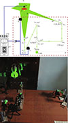 |
Figure 1. Experimental setup for the speckle interferometer. The letters in the schematic refer to driver with stinger (Dr), violin (V), acquisition system (AS), wave generator (WG), power amplifier (PA), computer (PC), Lumix camera (c1), webcam (c2), divergent lens (L), mirror (m), non-polarizing Beam Splitter (NPBS), pinhole aperture (AP), horizontal polarizer (P), laser (LAS), table ([0.5ex]0.15cm1.5pt[0.5ex]0.15cm1.5pt), digital wire ([0.5ex].25cm1.9pt), laser beam ([0.5ex].25cm1pt), angle between the beams (θ), cartesian reference frame (⋅ ⋅ ⋅). Suppl2.mp4 has a record of this setup working at the end of the video. |
If the intensity of each beam used for the illumination is I1 and I2 respectively, the resulting intensity Iref is then given by
 (1)
(1)
When the plane undergoes out-of-plane vibration, the phase modulation ξ induced by the vibration is
 (2)
(2)
where λ is the wavelength of the illuminating light and Δy is the amplitude of the normal displacement of the x − z plane. The intensity is modulated by a zeroth-order Bessel function, which is a standard operator readily available in numerical libraries, yielding
 (3)
(3)
The time-averaged speckle interferometry (TBSI) signal is then obtained as
 (4)
(4)
Equations (1)–(4) show that TBSI involves the digital subtraction of two interferograms. One is obtained from the speckle field produced by two coherent sources illuminating the object at rest, I ref. In the second, I vib, 1, the only change is that the object is set into vibration while maintaining the illumination that generated the initial speckle field unchanged throughout the measurement. This configuration is difficult to achieve without appropriate experimental optics facilities.
The decorrelated approach (DTBSI) is constructed by introducing a decorrelated phase shift Δϕ, meaning that an additional phase offset has occurred in the speckle field, leading to a second vibrational state
 (5)
(5)
from which the corresponding interferometric image is computed as
 (6)
(6)
Equations (5) and (6) show that DTBSI does not compare a stationary state with a vibrating state under the same speckle field, as in TBSI. In DTBSI, the relevant variation occurs in the phase of the speckle field: note that the only difference between equations (3) and (5) is the introduction of Δϕ. This implies that, in DTBSI, the speckle field is deliberately allowed to vary slightly between interferograms. Analytically, this variation is accounted for by including the parameter Δϕ in equation (5). Experimentally, the required variation typically arises naturally due to the practical difficulty of maintaining the relative positioning between the illuminating beams and the vibratory setup outside a controlled optical laboratory environment.
A code was written for Python (Suppl1.zip) following the order of the equations above, and all the required files to run it are available for download with this paper. The parameters for adjustments are λ, θ, Δϕ, intensity of the beams, the amplitude of the mode shape, and the speckle per centimeter. All the analytical interferograms in Section 5 were generated through this code.
Note that by defining Ω = (1 − cosθ)ξ, the fringe formation can be expressed in a well-known form in terms of Bessel functions. Equation (4) is governed by 1 − J 0(Ω), which produces dark nodal fringes in TBSI. In contrast, equation (6) leads to a response proportional to |J 0(Ω)|, yielding bright nodal fringes in DTBSI. This distinction is essential for interpreting the vibrational patterns, as it determines the fringe contrast and the visual representation of the deflections. However, in the code, equations (4) and (6) are implemented directly on a frame-by-frame basis, emulating the experimental procedure. As a result, the interferograms produced by the code exhibit the characteristic granular appearance of experimental data, which is smoothed out when the analytical interferograms are computed using the compact formulation provided by the Bessel functions.
3 Experiment
The optical arrangement mounted in the present work (diagram and actual devices in Fig. 1) was based on the DTBSI proposed by Moore et al. [9]. Some components of the optical setup must be selected with utmost care, while others are less critical. If the type of laser device and/or the beam splitter cube are not appropriate, the experiment will never work. The specifications of the mirrors are somewhat more flexible. The choice of lenses for beam expansion does not pose a significant challenge.
The laser used for the experiment was a diode-pumped solid-state device, see its suitability for interferometry in Section 3.3. A polarizer was used to determine the preferential polarization of the laser device; based on this information, the laser was rotated around its axis until its vertically polarized light was maximized. This adjustment was made because, in this interferometric configuration, vertical polarization enhances the fringe contrast. Finally, the polarizer was placed at the laser output to block the undesired horizontal polarization.
3.1 Beam paths
The next stage was beam splitting, but it was indispensable to preserve the same polarization in both beams. This point is worth emphasizing because, in standard beam splitter cubes, the polarization of the reflected beam rotates by 90°, whereas the transmitted beam maintains its original polarization. Consequently, a standard cube beam splitter does not work for a speckle interferometer. The experiment requires the use of a non-polarizing beam splitter cube (NPBS), which is more expensive than standard ones. Nevertheless, the 25 mm NPBS used here was newly acquired for US$ 50, a quite affordable price considering that one twice its size costs nearly five times more.
For correct interferometer operation, the Optical Path Difference (OPD) of the beams split from the NPBS must lie within the coherence length of the laser source, which is a critical requirement [9]. Even if the available laser has a coherence length long enough to neglect this issue, a safe procedure is to match the OPD to ensure compatibility with other laser sources.
To properly position the optical elements on the table and achieve equal OPD, a relation was derived to link known and unknown distances. The corresponding layout is shown in Figure 1. By mounting m1 and m2 such that  and θ ≈ 60° (where the overline denotes the distance between elements), the placement of the remaining components was constrained to satisfy
 (7)
(7)
The mirrors used for guiding the laser beams were not conventional glass mirrors; but flat, first-surface types. Four were required, two for each divided beam. Each one of these beams was expanded using divergent lenses. It was not necessary for the lenses used in each beam to be identical. In fact, for the beam perpendicular to the vibrating surface, a less-divergent lens was deliberately used than for the oblique beam. This ensures that the oblique beam reaches the vibrating surface with greater intensity, since the light barely covered the violin and was therefore more focused. This is advantageous, as higher intensity in the oblique beam improves interference.
Immediately after the beam-expanding lens, a pinhole aperture plate (AP) was placed. This plate blocks residual reflections from the mirrors, preventing them from reaching the violin. Although the setup described in [9] did not mention the use of an AP, its inclusion improves the original experiment and is straightforward to implement. The photograph in Figure 1 shows the unwanted laser light being blocked by the AP at the lens exit.
3.2 Phenomenon capture
A Panasonic Lumix DMC-FZ300 camera (c
1 in Fig. 1) was used to take the photographs. The exposure time was  s, f/8, ISO 1600, with optical zoom adjusted so that the violin body filled the limits of the photographic area. Additionally, a generic 4MP HD webcam (c
2 in Fig. 1), with a resolution of up to 1920 × 1080, was selected for the experiment. The only indispensable feature for its selection was manual focus. No zoom, digital or optical, was applied, so the violin occupied slightly less than one-fourth of the sensor’s image area. In both cameras, the plane of focus was the vibrating surface to be visualized. The cameras were not connected simultaneously.
s, f/8, ISO 1600, with optical zoom adjusted so that the violin body filled the limits of the photographic area. Additionally, a generic 4MP HD webcam (c
2 in Fig. 1), with a resolution of up to 1920 × 1080, was selected for the experiment. The only indispensable feature for its selection was manual focus. No zoom, digital or optical, was applied, so the violin occupied slightly less than one-fourth of the sensor’s image area. In both cameras, the plane of focus was the vibrating surface to be visualized. The cameras were not connected simultaneously.
The algorithm for real-time capture and visualization of the interference phenomenon was implemented in Python. It is available as supplemental material of this paper (Suppl3.py). The program captures an initial reference image and then calculates its absolute difference against each of the subsequent captured images. The reference image can be acquired with the object at rest; however, improved results were obtained when the reference corresponded to a vibrating state. The processed interferogram was displayed live on the screen. Upon stopping the program, the last 80 interferograms were saved.
Real-time control of the visualization was implemented by adjusting several parameters via the keyboard, including contrast, brightness, frames per second (FPS), the number of frames used to refresh the reference, and exposure. Stroboscopic sampling, achieved by synchronizing the image acquisition rate with the excitation frequency, is particularly useful for stabilizing the live image displayed during the experiment.
For example, for an excitation frequency of 170 Hz, setting the capture rate to 17 FPS ensures that images are acquired at a fixed phase of successive vibration cycles, resulting in a significantly more stable interferometric pattern than that obtained with unsynchronized acquisition. Additionally, freezing an appropriate dynamic reference acquired while the instrument was vibrating, at a phase state producing high-contrast fringes, significantly enhanced real-time visualization.
3.3 Testing laser coherence
Some lasers are unsuitable for producing interference patterns due to coherence issues, as it is explained in [13]. The minimum quality required for interferometry is achieved by a diode-pumped solid-state laser. Even so, it must be considered that the coherence of this type of laser is also limited and decreases with temperature oscillations. A laser of these characteristics was used: a Spyder III Krypton (532 nm). It is a relatively inexpensive device (US$499) compared to a laboratory laser, but the suitability for interferometry of its coherence length must be tested.
A proper coherence length of the laser here used was verified modifying the experiment depicted in Figure 1, until achieving the Michelson-like interferometer shown in Figure 2. m2 and m3 preserved their positions as in Figure 1, while c2 was relocated. Additional elements were incorporated. The no polarizing beam splitter NPBS was substituted for a polarizing version BS. m5 is a manually movable mirror to be located at the same distance between m2 and BS. L3 is a lens to expand the recombined beam towards the observation screen OS.
Figure 2 also includes the two images of the interference patterns captured by the webcam. Each image was labelled according to the interferometer arm used. When the OPD of the splitted beams was near zero, i.e. using the arms of 27 cm length, no fringes appeared. On the other hand, using the arm longer by 62 cm, dark fringes clearly appeared. It guaranteed a coherence of more than one meter (2 × 62 cm) of the laser, although the video showing this experiment (Suppl4.mp4) exhibited flicker during both OPD configurations. Even so, the performance of this laser allowed to neglect the variable beam distance across the surface when the violin was measured using the speckle setup of Figure 1.
 |
Figure 2. Schematic diagram of a Michelson-like interferometer used to explore the coherence length of the diode-pumped solid-state laser. m 2 and m 3: fixed mirrors as in Figure 1. m 5: manually movable mirror. BS: polarizing beam splitter. L 3: lens. OS: observation screen. c 2: camera. The images were labelled with the arm used to interfer. A video of this experiment showing the interferences is available in Suppl4.mp4. |
4 Top plate and violin as vibratory systems
The mode shapes targeted for interferometric sensing often are used as reference in violin acoustics (see [5–8, 14] as a few examples). On the one hand, modes 1, 2, and 5 were targeted for measurement on the plate. On the other hand, three signature modes were measured on the violin, namely CBR, B1−, and B1+. The first structure to be measured was a complete violin. The second structure was a complete violin top plate, including the f-holes, bass bar, and final thickness graduation. Both vibrating structures (hereafter referred to as the vibrating structures) were made of traditional violin-making woods and left unvarnished to enhance laser light reflection and promote the characteristic speckle phenomenon.
4.1 Mounting settings for interferometric sensing
The plate and violin were not mounted on the same table as the optical setup for the final arrangement described here (see Fig. 1), implying conditions for DTBSI. Besides, when the vibratory system was mounted on the same table as the optical system, the motion sensed by the interferometer did not correspond to flexural modes; instead, the excitation applied to the violin was transmitted to the table, and only rigid-body movements of the instrument were sensed, oscillating with the motion of the entire table. These rigid modes were revealed by parallel interference fringes, as shown in Figure 3. These fringes indicated that the system could already produce interference properly, but that the vibratory system was not adequately controlled.
 |
Figure 3. Fringes on the back plate of the violin revealing rigid motion of the whole system when the vibratory system was mounted on the same table of the optical devices. |
The solution to the rigid-body movements of the violin was to separate the vibratory system from the optical table. The vibrating structures were fixed to a bookshelf of approximately 200 kg using a frame designed for this purpose; additionally, the speaker without its cone used as an exciter was also mounted on the same bookshelf. To achieve proper visualizations, ensuring that the structure’s motion is exclusively the motion of interest is a crucial and delicate step. This meant that the only movements present were caused by deflection of the parts, and not by displacement of the entire structure.
Therefore, the vibrating structures were mounted mechanically isolated from the optical setup. Both structures were constrained so as to approach free boundary conditions, using specially designed supports. Each vibrational mode required a specific clamping pressure and excitation point. Figure 4 shows the base support for mounting the vibrating structures.
 |
Figure 4. Holding the plate using a thread through f-holes (a) and sponges on the back (b). |
Two modular aluminum extrusion rails with several adjustable-position screws were used to hold the plate. The rails were green painted to avoid undesirable laser reflections. The plate was suspended by a thread passed through the f-holes and routed across the front (Fig. 4a). On the back side, three pieces of low-impedance material (sponges) gently pressed against expected nodal lines of the mode to be visualized (Fig. 4b). The plate was not resting on the base.
The violin was supported on the same structure used for the plate, but in a completely different manner. Restricting undesirable rigid-body motions of the violin while allowing the relevant vibrational modes is challenging. To minimize perturbations of the mobility, the violin was mounted following the recommendations described in [5]. It was secured using screws at four points: two at the upper block and two at the lower block (see details in Figs. 1 and 4). The screw pressure was kept to the minimum required to prevent sliding when the instrument was gently nudged by hand. After measuring the three operational deflection shape (ODS) by visualizing the violin top plate, the instrument was rotated to visualize the back plate.
Impulse sound responses were rapidly measured to determine appropriate fixation and excitation conditions for the ODS to be visualized. The vibrating structures were tapped by finger at expected antinodal regions on their back sides. Simultaneously, the generated sound was sensed with a microphone placed near an expected antinodal region of the mode. Therefore, the sound response was calculated. Clamping pressure and excitation point were varied while monitoring the sound response, with the objective of obtaining a pronounced peak at the expected resonant frequency. A low peak indicated an overdamped mode that would be difficult to visualize.
The structures were mechanically excited at the point where the sound response exhibited the highest peak at the resonant frequency of interest. For this purpose, a 4-inch loudspeaker was modified by removing its cone to avoid airborne sound radiation and mounting a stinger directly on the voice coil. The loudspeaker was driven by a Yamaha P7000S amplifier. A computer supplied a sinusoidal signal at the target modal frequency, determined from the previously measured sound response. Careful control of the excitation amplitude was essential to visualize the interference fringes, and each mode required an individual exploration to determine the appropriate excitation level.
4.2 Modal testing
Although the low-order modes of the violin and the plate exhibit clearly separated resonant peaks and are generally well documented in the literature, it should be noted that measurements obtained with the interferometer still correspond to ODS of the specific structures under study. For this reason, both the violin and the plate used in the interferometric measurements were subjected to experimental modal analysis under conditions close to free boundary conditions. The modal parameters were extracted to be compared with those obtained from the interferometric setup, which requires significantly more rigid mounting conditions.
Each vibrating structure was measured by exciting it at a fixed point using a Brüel & Kjær mini impact hammer operated as a pendulum. The plate was mounted by suspending it using two threads through the f-holes, aiming to approximate free boundary conditions. The excitation point was located near the edge at one of the lower corners, between an expected nodal line of mode 2 and the plate symmetry line. The violin was placed vertically resting on rubber bands at bottom, and holding the neck using another rubber band. The violin was excited at the bass corner of the bridge, following the classical setup for bridge mobility measurements [15].
The dynamic response of the vibrating structures was sensed by attaching a Kistler ultra-miniature accelerometer (0.4 g) using wax, while performing a point-by-point scan over a 2 cm grid covering the structures. The measured signals were conditioned and processed to obtain a transfer function (velocity/force) at each spatial location. The mode shapes calculated through modal testing were obtained using Python. Mode extraction was performed using the peak-picking method [16]. The mode shapes obtained were used as the vibrating data read to calculate the analytical interferograms.
5 Results
Several data from different sources were analyzed: analytical calculations for interferometry, a finite element simulation of a plate, experimental modal analysis, and experimental interferometry; which in turn, was taken using two different cameras. Each interferogram was recorded in a single experimental session adjusting specific parameters to improve the visualization.
5.1 Testing the algorithm applied to modal data
Firstly, the performance of the analytical interferometry model described in Section 2 was verified. For this purpose, the experimental setup used to record the interferograms reported in [9], corresponding to a high-frequency mode of a 24 cm isotropic square plate fixed at the center, was modeled. This mode shape was obtained from a finite element model of the plate, while the speckle field was approximated using random noise. The TBSI and DTBSI interferograms (Fig. 5), calculated by the code in Suppl1.zip, are in agreement with the corresponding experimental results reported in [9]. The expected dark nodal lines of TBSI were obtained, whereas DTBSI exhibited a different sensitivity of the contour fringes and cannot be interpreted as a simple contrast inversion of TBSI. In these analytical interferograms, the granular appearance arises from the actual interference of the simulated speckle field, as in the real interferometer, and is not superimposed on smooth fringe functions. Hereafter, these will be referred to as analytical interferograms.
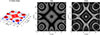 |
Figure 5. Analytical interferograms calculated using an adjustable Python code implementing equations (1)–(6) (Suppl1.zip), in which random noise is used to simulate the speckle field that undergoes interference. The results correspond to a mode shape of a square plate fixed at the center, obtained from a finite element model, and show agreement with the experimental counterpart reported in [9]. |
5.2 Interferograms using the Lumix camera
Figure 6 show the experimental and analytical interferograms of the violin v517. The experimental versions (left) are typical captures of the ODS of the violin using the Lumix camera. The flexibility of the Lumix camera settings allowed testing different combinations of f-number, exposure time, and ISO, making it possible to obtain some high order fringes in each ODS. The only processing applied was converting the images to grayscale, which is performed in real time while the experiment is running.
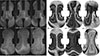 |
Figure 6. Interferograms showing the top and back plates of three signature modes in the violin v517: CBR, B1−, B1+. Right: analytical interferograms from experimental modal data. Left: Lumix camera capturing ODS at the indicated frequency. Suppl2.mp4 is a video containing typical sessions measuring interferograms at these frequencies. |
The comparison of the ODS obtained using the Lumix camera against the analytical interferograms derived from the experimental mode shapes revealed additional experimental details. The ODS corresponding to CBR and its frequency appears to be largely unaffected by the mounting conditions used for the optical measurements. For the B1 modes, the clamping method introduced slight variations in the nodal lines; however, as in the case of CBR, the signature modes remain clearly identifiable. The frequency of B1+ exhibited a significant shift of 13 Hz.
Separating the vibrating structures from the optical table was sufficient for the experiment to operate under DTBSI conditions, as evidenced by the characteristic white nodal lines associated with DTBSI. Nevertheless, it is noteworthy that the experimental interferogram of the back plate at 538 Hz may not be decorrelated, since its fringe pattern more closely matches the analytical TBSI version (black nodal lines). In Figure 6, all analytical interferograms correspond to the DTBSI formulation, except for the back plate at 525 Hz (see Fig. 7 for the DTBSI version).
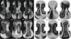 |
Figure 7. Interferograms showing the top and back plates of three signature modes in the violin v517: CBR, B1−, B1+. Right: analytical interferograms from experimental modal data. Left: webcam capturing the operational deflection shape at the indicated frequency. Suppl2.mp4 is a video containing typical sessions measuring interferograms at these frequencies. |
5.3 Interferograms using the webcam
The ODS shown in Figure 7 were obtained using the webcam, and a recalculation of the DTBSI version of the analytical interferograms was included. The fringes obtained are thicker than those in the ODS captured with the Lumix camera (Fig. 6). The amplitude of the mode shapes used to recalculate the analytical interferograms had to be reduced to avoid the appearance of higher-order fringes. It is also observed that the fringes exhibit higher contrast, even though the webcam settings are limited to basic control of the exposure time.
Finally, Figure 8 shows the interferograms of the free top plate in real time using webcam images, without any additional processing; Suppl5.mp4 is a video showing the three experimental sessions in which these modes were extracted. The bright fringes in the experimental ODS followed closely the mode shapes of the analytical interferograms without altering the modal frequency. Therefore, the setup designed to hold and excite the top plate proved to be close to free conditions for this type of optical testing.
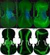 |
Figure 8. Interferograms of the first, second, and fifth free mode shapes of a violin top plate. Bottom: analytical interferograms from experimental modal data. Top: webcam capturing the operational deflection shape at the indicated frequency. supp5.mp4 is a video created from the sessions in which these modes were extracted. |
The analytical interferograms predicted the presence of higher-order fringes for the nodal line widths revealed by the experimental interferograms. However, these same analytical interferograms exhibited limited contrast outside the nodal lines. It is possible that the dynamic range of the webcam was insufficient to clearly resolve such fringes, as appears to be the case in the lower region of the plate for the first and second modes (see Fig. 8 and Suppl5.mp4). Additionally, inherent experimental limitations, such as the aforementioned laser flicker or the violin geometry, may also be contributing factors to this issue. For instance, the blue pixels indicate luminance saturation in the camera caused by the plate arching. Specifically, at these blue pixel locations, the surface curvature allows the plate to receive light more directly from the oblique arm.
6 Conclusions
An interferometric system capable of operating without specialized optical equipment or controlled laboratory conditions has been successfully developed and validated for violin acoustics. The experimental results demonstrate that reliable interferometric measurements can be achieved under non-ideal conditions, significantly expanding the practical applicability of the technique.
A key result is the good agreement observed between the experimentally obtained interferograms and those analytically reconstructed from mode shapes obtained through experimental modal analysis. Also, the analytical version of the interferometer allowed a quick exploration of different configurations by adjusting parameters as laser color, angle between beams, amount of decorrelation, mode shape amplitude, and speckle size.
Additionally, the proposed implementation achieves a significant reduction in cost compared to conventional interferometric setups. This aspect is critical for enabling the adoption of interferometric techniques in non-specialized environments, such as educational settings or resource-limited laboratories.
From a pedagogical perspective, the accessibility of the system, combined with the availability of experimental data, visualization videos, and Python codes, provides a valuable platform for teaching fundamental concepts in wave interference, modal analysis, and structural dynamics. This facilitates a more intuitive and interactive understanding of interferometric principles, bridging the gap between theoretical formulations and experimental observation.
In fact, it is prudent to emphasize that constructing an experimental speckle interferometer as presented here, from scratch, is not a simple one-week project. This point is worth mentioning because the first impression one might have when inspecting the original setup [9] is that it would be straightforward. Although the analytical version of the interferometer reading modal experimental data offers an interesting alternative for exploration, having a real optical system permanently available in an acoustics laboratory is useful not only as a tool but also for the momentum it generates in both research and teaching: seeing the system in operation immediately sparks student interest, as it is common for them to have encountered violin interferograms in various papers and books on violin acoustics.
Although the primary objective of designing a functional interferometer for violin acoustics has been achieved, significant opportunities for further investigation remain. Future work will focus on improving the system not only through hardware upgrades (such as a more suitable laser and a camera with a higher-performance sensor), but primarily by developing a deeper understanding of its operation through systematic experimental use. This approach is expected to extend the measurement capabilities toward more advanced studies of violin vibrations, including higher-order modes, traveling wave phenomena, and transient analysis.
Acknowledgments
The author acknowledges Johenelly Madrigal, Rodrigo Arboleyda, and Carlos Torres Torres for the donation of equipment used to set up the experiment; the students of the Escuela de Laudería INBAL for their support at different stages of the experiment; and Thomas Moore for his comments during the development of the early versions of the interferometer.
Conflicts of interest
The authors declare no conflict of interest.
Data availability statement
Data are available on request from the authors.
Supplementary material
Suppl1.zip contains the python code and the required files to calculate the analytical interferograms for the finite element model of a plate, and for the experimental modal analysis of the same violin and top plate measured using the interferometer.
Suppl2.mp4 is a video of the interferences of the violin using the Lumix camera and the webcam; a record of the experimental setup working was included at the end.
Suppl3.py is the python code here developed to handle any camera and to interfere the acquired images.
Suppl4.mp4 is a video showing the Michelson interferometer used to test the performance of the laser device.
Suppl5.mp4 is a video showing the interferences of the three modes studied in the free top plate using webcam.
Access Supplementary MaterialReferences
- W. Reinicke, L. Cremer: Application of holographic interferometry to vibrations of the bodies of string instruments. Journal of the Acoustical Society of America 48, 4B (1970) 988–992. [Google Scholar]
- E. Jansson, N.-E. Molin, H. Sundin: Resonances of a violin body studied by hologram interferometry and acoustical methods. Physica Scripta 2, 6 (1970) 243. [Google Scholar]
- N.-E. Molin, A.O. Wahlin, E.V. Jansson: Transient wave response of the violin body. Journal of the Acoustical Society of America 88 (1990) 2479–2481. [Google Scholar]
- N.-E. Molin, A.O. Wahlin, E.V. Jansson: Transient wave response of the violin body revisited. Journal of the Acoustical Society of America 90 (1991) 2192–2195. [Google Scholar]
- A. Runnemalm, N.-E. Molin, E. Jansson: On operating deflection shapes of the violin body including in-plane motions. Journal of the Acoustical Society of America 107, 6 (2000) 3452–3459. [Google Scholar]
- J.A. Torres, L.-D. Canales-Hernández, P.A. Acosta, J.-J. González-Barbosa, J.-B. Hurtado-Ramos: Vibrations of a violin while the f-holes were sequentially cut. Acoustics Australia 52, 1 (2024) 95–103. [Google Scholar]
- S.D. Bellows, D. Nakayama: An investigation of the f-hole shape’s influence on the modal response of the violin. Acta Acustica 8 (2024) 67. [Google Scholar]
- A. Meza-Pérez, G. Stoppani, R. Viala, S. Gonzalez, U. Igartua, R. Jardón Rico, C. Fritz: Towards a finite element model of a batch of experimental violins: validation on sub-structural components. Acta Acustica 9 (2025) 2. [Google Scholar]
- T.R. Moore, A.E. Cannaday, S.A. Zietlow: A simple and inexpensive optical technique to help students visualize mode shapes. Journal of the Acoustical Society of America 131, 3 (2012) 2480–2487. [Google Scholar]
- J.A. Torres: Open source application for mobility measurements on violins. Computer Applications in Engineering Education 26, 5 (2018) 1111–1119. [Google Scholar]
- J.A. Torres, C.A. Soto, D. Torres-Torres: Exploring design variations of the Titian Stradivari violin using a finite element model. Journal of the Acoustical Society of America 148, 3 (2020) 1496–1506. [Google Scholar]
- J.A. Torres, C. Torres-Torres, E. Vidal, F. Fernández, M. de Icaza-Herrera, A.M. Loske: Violin vibration state determined from laser streak patterns. Applied Acoustics 185 (2022) 108384. [Google Scholar]
- Y. Salvadé, R. Dändliker: Limitations of interferometry due to the flicker noise of laser diodes. Journal of the Optical Society of America A 17, 5 (2000) 927–932. [Google Scholar]
- E. Skrodzka, A. Krupa, E. Rosenfeld, B. Linde: Mechanical and optical investigation of dynamic behavior of violins at modal frequencies. Applied Optics 48, 7 (2009) C165–C170. [Google Scholar]
- E.V. Jansson: Admittance measurements of 25 high quality violins. Acta Acustica United with Acustica 83, 2 (1997) 337–341. [Google Scholar]
- D.J. Ewins: Modal Testing: Theory and Practice. Research Studies Press, Letchworth, 1984. [Google Scholar]
Appendix A
Some details about settings
Figure 1 shows the experimental setup, where each component can be examined as a complement to the explanations provided in this appendix. The experimental assembly began with the selection of a suitable installation site. The location had to be capable of being completely darkened. Additionally, the floor needed to be as resistant to deformation as possible.
A 183 cm × 91 cm office desk was used to mount the optical system. The drawers were filled (wood, loudspeakers, etc.) to increase its mass. A folded 2 mm neoprene strip was placed under each of the four legs to dampen floor contact. All elements were firmly screwed to the desk. The desk was leveled horizontally, although this was not strictly required, nor was a perfectly flat working surface.
On the other hand, proper operation of the system requires that the beams be strictly coplanar. This condition ensures
that the wavefronts reach the interference region with identical geometry and propagation direction, thereby guaranteeing correct collimation. A laser level (Bosch GLL 12-22 G) and several bubble levels were used to facilitate this alignment. Although preliminary versions of the experiment achieved acceptable collimation without a laser level, its use is strongly recommended, as it significantly accelerates the procedure.
Designing functional mechanical systems to hold the optical elements required considerable effort, since, as shown in Figure 1, virtually no standard optical mounts were available. Involving students in these designs fostered a positive sense of participation in the project. Table A.1 lists how commercial devices were replaced by lower-cost alternatives to achieve a significant cost reduction. The column describing the mounting method can be complemented by inspection of Figure 1.
Low-cost alternatives to specialized optical testing components, avoiding an estimated total investment of approximately US$1504 in equivalent entry-level commercial devices. This estimate does not include the mandatory investment in the laser source (approximately US$500 for the Spyder Wicked model used here), the non-polarizing beam splitter (approximately US$54), or the generic data acquisition system (camera and computer).
Cite this article as: Torres J.A. 2026. Designing a speckle interferometer for violin acoustics. Acta Acustica, 10, 54. https://doi.org/10.1051/aacus/2026041.
All Tables
Low-cost alternatives to specialized optical testing components, avoiding an estimated total investment of approximately US$1504 in equivalent entry-level commercial devices. This estimate does not include the mandatory investment in the laser source (approximately US$500 for the Spyder Wicked model used here), the non-polarizing beam splitter (approximately US$54), or the generic data acquisition system (camera and computer).
All Figures
|
Figure 1. Experimental setup for the speckle interferometer. The letters in the schematic refer to driver with stinger (Dr), violin (V), acquisition system (AS), wave generator (WG), power amplifier (PA), computer (PC), Lumix camera (c1), webcam (c2), divergent lens (L), mirror (m), non-polarizing Beam Splitter (NPBS), pinhole aperture (AP), horizontal polarizer (P), laser (LAS), table ([0.5ex]0.15cm1.5pt[0.5ex]0.15cm1.5pt), digital wire ([0.5ex].25cm1.9pt), laser beam ([0.5ex].25cm1pt), angle between the beams (θ), cartesian reference frame (⋅ ⋅ ⋅). Suppl2.mp4 has a record of this setup working at the end of the video. |
| In the text | |
|
Figure 2. Schematic diagram of a Michelson-like interferometer used to explore the coherence length of the diode-pumped solid-state laser. m 2 and m 3: fixed mirrors as in Figure 1. m 5: manually movable mirror. BS: polarizing beam splitter. L 3: lens. OS: observation screen. c 2: camera. The images were labelled with the arm used to interfer. A video of this experiment showing the interferences is available in Suppl4.mp4. |
| In the text | |
|
Figure 3. Fringes on the back plate of the violin revealing rigid motion of the whole system when the vibratory system was mounted on the same table of the optical devices. |
| In the text | |
|
Figure 4. Holding the plate using a thread through f-holes (a) and sponges on the back (b). |
| In the text | |
|
Figure 5. Analytical interferograms calculated using an adjustable Python code implementing equations (1)–(6) (Suppl1.zip), in which random noise is used to simulate the speckle field that undergoes interference. The results correspond to a mode shape of a square plate fixed at the center, obtained from a finite element model, and show agreement with the experimental counterpart reported in [9]. |
| In the text | |
|
Figure 6. Interferograms showing the top and back plates of three signature modes in the violin v517: CBR, B1−, B1+. Right: analytical interferograms from experimental modal data. Left: Lumix camera capturing ODS at the indicated frequency. Suppl2.mp4 is a video containing typical sessions measuring interferograms at these frequencies. |
| In the text | |
|
Figure 7. Interferograms showing the top and back plates of three signature modes in the violin v517: CBR, B1−, B1+. Right: analytical interferograms from experimental modal data. Left: webcam capturing the operational deflection shape at the indicated frequency. Suppl2.mp4 is a video containing typical sessions measuring interferograms at these frequencies. |
| In the text | |
|
Figure 8. Interferograms of the first, second, and fifth free mode shapes of a violin top plate. Bottom: analytical interferograms from experimental modal data. Top: webcam capturing the operational deflection shape at the indicated frequency. supp5.mp4 is a video created from the sessions in which these modes were extracted. |
| In the text | |
Current usage metrics show cumulative count of Article Views (full-text article views including HTML views, PDF and ePub downloads, according to the available data) and Abstracts Views on Vision4Press platform.
Data correspond to usage on the plateform after 2015. The current usage metrics is available 48-96 hours after online publication and is updated daily on week days.
Initial download of the metrics may take a while.