© The Author(s), Published by EDP Sciences, 2026

1 Introduction

The study of sound propagation in moving fluids is relevant to a wide range of physical problems and applications, including outdoor sound propagation [1, 2], underwater acoustics [3], and various industrial processes [4].

In sound applications over short-range distances, high-frequency sound propagation models can be used in investigating how sound waves propagate and interact with flowing fluid e.g. in underwater applications [5], medical imaging (e.g., ultrasound) [6], and flow measurement in pipelines (e.g., ultrasonic flow meters) [7].

The movement of the fluid itself can alter the acoustic waves in such cases, depending on the flow velocity, the flow profile and the speed of sound profile. Therefore, the study and understanding of how these effects can impact on the sound wave propagation along a desired acoustic path remains relevant for practical applications where high flow velocities are in use, such as ultrasonic flow meters [4, 7] hereinafter referred to as USM.

USMs based on the transit-time difference principle, have become increasingly more relevant for measurement of pipe flow of single-phase liquid or gas [4, 7]. They are currently used e.g. for process control measurements, emission measurements and even in custody transfer applications. Thus, possible loss of accuracy of the measurements by USMs caused by the interaction between the flow and the acoustic wave may have large practical and economic impacts in given applications.

The operational principle of USMs is based on pairs of ultrasonic transducers aligned opposite to each other across the pipe. Acoustic pulses are sent back and forth between the transducers, across the fluid stream to be measured [4, 8, 9]. As sound waves travel faster with the flow direction than against the flow direction, a transit time difference is found between the acoustic pulse propagating upstream and the one propagating downstream. The transit time difference is used for determination of the average flow velocity across the straight line between the two transducers. This straight line will hereafter be denoted the acoustic path.

As the flow velocity varies over the pipe cross-section, the USM must be able to perform accurate flow velocity measurements over a wide range of flow profiles. This is done by applying several pairs of ultrasonic transducers. Thereby, the average flow velocity is measured over several acoustic paths. These measured flow velocities are thereafter combined into an average flow velocity over the whole pipe cross-section.

To mitigate the effect of flow on USM measurements, various techniques have recently been investigated. These include use of specialized transducers and signal processing algorithms [10, 11] and theoretical design and computational fluid dynamics of transit-time USMs to improve measurement accuracy [12], and flow field simulation on the pipeline of a single-phase USM [13] to identify the optimal transducer configuration. However, in order to further improve the accuracy of USMs, the study of flow effects on sound propagation on individual acoustic paths in USMs remains relevant.

The flow velocity calculation on individual acoustic paths relies on a simplified plane wave model using an effective speed of sound, which does not account for acoustic beam effects caused by finite-sized transducers and their interaction with the flowing gas. Diffraction effects can be corrected for, but available correction formulas apply only to non-flowing fluids. The distance between the transmitter and receiver was shown to have an impact in early studies of sound velocity and attenuation in different media [14–16]. A model to explain these effects of transducer diffractions, based on the model for a baffled uniform piston transducer was presented by Williams [17]. Diffraction corrections for a stagnant fluid were then carried out by taking the average free-field pressure over the receiver front surface [18, 19].

Several papers based on diffraction corrections in a motionless fluid following these early investigations are relevant. An approach to describe the diffraction correction of an acoustic receiver located in the sound field of a non-uniformly vibrating and finite-sized transmitting transducer was proposed in [20, 21] as an improved but still simplified approach to account for such effects.

Further to the points discussed above, a finite element method was used to implement the piezoelectric transducer vibrations, the resulting sound field and diffraction corrections, such as an unbaffled piezoelectric transducer operating in gas across its relevant frequency band and vibration modes [21–23]. The resulting complex diffraction correction was compared with the classical baffled piston model approach, showing significant deviations from the piston diffraction correction for different vibration modes of the transducer. All these previous works were conducted in a motionless fluid, highlighting the need for further work on diffraction effects in flowing fluid for USM applications.

As the fluid flows at an angle relative to the acoustic path, the acoustic beam will tilt in the flow direction. This effect was previously studied using simple geometrical models in [24]. However, to the authors knowledge, no study has yet combined the flow velocity profile with diffractions of the acoustic beam in a fully consistent manner based on the fundamental equations governing wave propagation under such conditions. Consequently, the combined effect of acoustic beams and flow on the propagation of ultrasonic waves along acoustic paths should be investigated.

In literature, several models of relevance for ultrasonic flow meters have been derived and numerically implemented for this purpose, as seen in [13, 25–29]. They are based on methods like ray tracing [30, 31], or the linearized equations of fluid dynamics and the convected acoustic wave equation [31–33]. Ray tracing methods are well-established to understand and simulate the effects of flow profiles on sound waves, based on the principles of geometrical acoustics, which assume high-frequency waves [31–33]. However, simple ray tracing methods, typically cannot model sound diffraction.

Therefore, approaches such as convective wave equation [31, 32] or parabolic equations [31] may be more suitable as they can fully combine these two effects in their theoretical models. A linearized fluid dynamic equation [31, 32, 34] can be considered as well. However, the latter may not be fully implemented numerically due to the significant mathematical and computational costs involved. To reduce computational time, facilitate the interactions between flow and sound propagation and avoid numerical reflection from boundaries, parabolic equation approximations can be utilized. A particular emphasis is therefore put on parabolic equations as they are well suited to smaller computers, larger domains, higher frequencies and can handle diffraction and flow effects on sound beams over short range distances for low Mach number and/or small variations in the sound speed.

As a first step in such an investigation, the sound field generated by a uniform piston that radiates into a uniformly flowing homogeneous fluid was studied in [35] by using a parabolic equation. In the present work, this work is extended by applying a parabolic flow velocity profile characteristic of laminar flow. The difference between the sound fields propagating through a uniform and a parabolic flow velocity profile can then be studied. To the best of the authors’ knowledge, this has not been explored before.

It is important to emphasize that this study does not question the accuracy of current USMs nor aim to improve their metering performance. Instead, its purpose is to further investigate how the two effects discussed above influence the ultrasonic signal, potentially causing deviations and distortions in the sound-pressure field along the acoustic path.

This paper is outlined as follows. Firstly, we develop the theoretical model of the sound field through a laminar flow regime based on the operational principle of USMs by using a high-frequency, narrow-angle three-dimensional parabolic equation [31], including the effects of flow and diffraction effects. A solution of the parabolic equation in form of an integral is then established. Secondly, the acoustic trajectory essentially described by the main lobe of the sound field by use of this integral solution is compared to the ray trajectory in laminar flow based on the ray theory approach. Thirdly, a mathematical comparison of the acoustic wave through a uniform and a laminar flow regime is investigated through the integral solution. These results are supported by the ray theory approach. Finally, numerical simulations are presented to illustrate the mathematical results.

2 Theoretical method

2.1 Theoretical model

The theoretical model used here is a simplified version of the sound propagation along an acoustic path in a USM. However, the acoustic path is not oblique in our model.

Several assumption are made on the geometry and the flow, as listed in (i)–(iv) below.

• (i)

  The sound source is a uniform circular piston located in a flat baffle at z = 0. It radiates only into the half-space z >  0 at normal angle of incidence within a narrow angular range (typically less than 20°); Thus, it is assumed that the preferred direction of the beam propagation in the model is vertical from z = 0 to z = d, and will hereafter be referred to as the no-flow acoustic axis (see Fig. 1). The acoustic field is assumed to operate in the high-frequency regime, where the acoustic wavelength is much smaller than the piston radius.

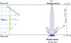
  Figure 1. Sketch of the geometric used in this paper.

• (ii)

  Two parallel planes are employed to mimic the internal pipe wall boundaries in the USM as sketched in Figure 1, with the aim of providing a framework for investigating the flow velocity profile within a pipe section. Reflections from these mimicked pipe walls are not taken into consideration. This means that we consider acoustic propagation from z = 0 to z = d with no wall reflection at z = d, see Figure 1. d is the pipe diameter.

• (iii)

  The flowing fluid is homogeneous and lossless (no acoustic absorption). Moreover, we assume that the fluid has no influence on the vibration of the piston.

• (iv)

  The flow is in the x-direction. A laminar flow velocity profile is applied. This means that the component of the flow velocity in the x-direction depends on z like

  $$\begin{array}{c}\hfill v_{0x}(z)=v_{\text{max}}(1-\frac{{(z-d/2)}^2}{{(d/2)}^2}),\end{array}$$(1)

  v _max is the maximum flow velocity, occurring at the centre of the pipe (z = d/2), see Figure 1. Note also that the flow velocity is zero at the pipe wall (z = 0 and z = d). This means that the pipe wall is not fully modelled but mimicked by the selected flow profile.

Due to the assumptions (i)–(iv), the acoustic path is not fully modelled as mentioned above. In addition to the explicitly stated assumptions, there is also an implicit assumption. In a real acoustic path in USMs, the direction of the acoustic propagation will form an angle of about 45 to 60 degrees to the flow direction, while here the direction of the acoustic propagation is perpendicular to the flow direction. This is selected as a simple set-up for studying the interaction between an acoustic beam and the flow. It can be a basis for future generalizations towards more realistic set-ups for acoustic paths in USMs and for others applications.

The acoustic propagation will be described by a linear high-frequency, narrow-angle three-dimensional parabolic equation with flow term included and no acoustic absorption. An approach using a parabolic equation is selected because of simpler numerical solution methodologies as mentioned previously. The full derivation of the parabolic equation is given in [31] by neglecting terms related to the pressure gradient in the direction perpendicular to the beam’s propagation, and the final equation is given as equation (2.111). Under assumptions (i)–(iv), it reduces to

$$\begin{array}{c}\hfill {\mathrm{\Delta }}_{\perp }{q}_{{}_L}(x,y,z)+2\frac{\text{i}k}{c}{v}_{0\perp }·{\mathrm{\nabla }}_{\perp }{q}_{{}_L}(x,y,z)+2\text{i}k\frac{\partial q_{{}_L}}{\partial z}(x,y,z)=0,\end{array}$$(2)

which is sought in Cartesian coordinates (x, y, z) for a sound beam generated by a uniform circular piston at z = 0 given by

$$\begin{array}{c}\hfill q_{{}_L}(x,y,0)=\{\begin{array}{cc}{\rho }_{0}c{\overline{v}}_s\hfill & \text{when}{x}^2+y^2<a^2,(\mathcal{L})\hfill \\ 0\hfill & \text{elsewhere},\hfill \end{array}\end{array}$$(3)

and where the acoustic pressure with angular frequency ω is p _L (x, t)=Re(e^{i(kz − ωt)} q _L (x)) and the index L hereinafter will be referred to the laminar flow velocity profile. k = ω/c is the wave number, c is the speed of sound. Δ_⊥ = ∂²/∂x ² + ∂²/∂y ² is the Laplacian in the lateral coordinates x and y, ∇_⊥ = (∂/∂x,∂/∂y), v _0⊥ = (v _0x ,v _0y ) is the horizontal component of the flow velocity where v _0y  = 0 and v _0x (z) are defined in equation (1). ρ ₀ is the ambient density of the fluid, and ${\overline{v}}_s$ is the amplitude of the uniform velocity of the sound source. ℒ is the surface of the uniform piston of radius a (constant).

The second term in equation (2) describes advection of an acoustic wave due to the flow velocity component perpendicular to the z-axis. If the flow velocity is set to zero, the second term in equation (2) vanishes and the equation is reduced to the well-known parabolic equation for sound waves in a homogeneous motionless fluid, as derived in [36] and in many textbooks in acoustics, with no dissipative terms included.

Note that the parabolic equation does not usually provide a good representation of the acoustic field at distances from the plane of the uniform piston of the order of a(ka)^1/3 ≡ L or less [36]. This means that equation (2) remains valid under the assumption z ≥ L.

Important orders of magnitude and paraxial approximations for small angle approximations are discussed in further depth in [31], which also takes into account multiple ranges of validity of equation (2). As studied in [31], these approximations are valid when the ka-number is large, the wave propagation is required in a narrow beam geometry not too near to the source, and when the fluid is homogenous. This also means that the narrow-beam approach is valid in a narrow angular range around the no-flow acoustic axis, like the traditional no-flow parabolic equation studied in [36], and is also valid in a narrow angular range around the bended beam due to flow velocity less or equals to 10 m/s as shown in [31]. This flow velocity above is significantly higher than the flow velocity range for laminar flow regimes applied in USM applications, which is at most about 1 or 2 m/s. However, solely for the sake of visualization of the sound pressure field along the acoustic path, this flow velocity range will be extended.

For the parabolic equation to be valid, low Mach number and/or small variations in the sound speed are assumed [31]. Omitting second-order terms pertinent to these quantities might result in insignificant phase errors for short propagation ranges. However, they might lead to significant cumulative phase errors for long propagation ranges [37, 38].

The flat uniform circular piston embedded in an infinite baffle vibrates uniformly in the normal direction. Applying this type of piston remains valid for low Mach number or stagnant and lossless fluid. However, under flowing conditions, its radiation pattern and energy distribution can be altered by the flow motion. Nevertheless, the piston-type model remains valid under the frozen-flow assumption for turbulent flows, as developed in [39].

This frozen-flow approach treats the fluid velocity field as fixed during the short acoustic propagation time. When the speed of sound is significantly greater than fluid motion (low Mach number), sound propagation can be simulated using a static snapshot of the flow field, thereby maintaining the validity of the uniform piston. Thus, the acoustic field emitted by the piston into that snapshot stays accurate during propagation [39], since the flow field does not change much in space or time near the piston and along a short propagation path. In line with this, the laminar flow is fully developed, deterministic and does not fluctuate or change over time. Therefore, the flow is already frozen in time.

2.2 The integral solution

Equation (2) combined with equations (1) and (3) can be solved by numerical methods like finite element method and method of lines. However, as in [35, 40] an exact solution can be written in terms of an integral. Thereafter, numerical solutions can be found from this integral.

The integral is developed by use of a two-dimensional spatial Fourier transformation in x and y coordinates that leads to an ordinary differential equation in the z-variable. The ordinary differential equation can be solved analytically and by applying inverse spatial Fourier transform in the x and y direction, a two-dimensional integral expression for the solution is found. It is expressed as

$$\begin{array}{cc}& q_{{}_L}(x,y,z)=\frac{k{\rho }_{0}c}{2\text{i}\pi z}{\text{e}}^{\text{i}kz\frac{M^2}{2}{\left(\frac{z}{d}\right)}^2{(3-\frac{z}{(d/2)})}^2}\hfill \\ \hfill & \times \int {\int }_{\mathcal{L}}{\text{e}}^{\frac{\text{i}k({(x-x_0)}^2+{(y-y_0)}^2)}{2z}}{\text{e}}^{-\text{i}kM\left(\frac{z}{d}\right)(3-\frac{z}{(d/2)})(x-x_0)}\hfill \\ \hfill & \times {\overline{v}}_s(x_0,y_0)\mathrm{d}{x}_0\mathrm{d}{y}_0,\hfill \end{array}$$(4)

where $M=\frac{v_{}\text{avg}}{c}$ is the flow Mach number, and the average flow velocity v _avg is calculated as follows

$$\begin{array}{c}\hfill v_{\text{avg}}=\frac{1}{\mathrm{d}}{\int }_0^d{v}_{0x}(z)\mathrm{d}z=\frac{2}{3}{v}_{\text{max}}.\end{array}$$(5)

To the authors’ knowledge, this solution has not been reported elsewhere. The derivation of equation (4) is given in Appendix A.

It is well-known that in the case of no flow, the sound beam generated by a uniform piston source has two characteristic quantities, characterized here by the ka-number and the Rayleigh distance ka ²/2. In equation (4), there will be more characteristic quantities due to the flow profile and the average flow.

This is illustrated by introducing non-dimensional coordinates x = ax′, y = ay′, $z=\frac{k{a}^2}{2}z\prime$ and $d=\frac{k{a}^2}{2}d\prime$. Equation (4) is then converted into

$$\begin{array}{cc}& q_{{}_L}(x^{\prime },y^{\prime },z^{\prime })=\frac{{\rho }_{0}c{\overline{v}}_s}{\text{i}\pi z^{\prime }}{\text{e}}^{\text{i}{(ka)}^2{M}^2\left(\frac{z^{\prime }}{4}\right){\left(\frac{z^{\prime }}{d^{\prime }}\right)}^2{(3-\frac{z^{\prime }}{(d^{\prime }/2)})}^2}\hfill \\ \hfill & \times \int {\int }_{{\mathcal{L}}^{\prime }}{\text{e}}^{\frac{\text{i}}{z^{\prime }}[{(x^{\prime }-x_0^{\prime })}^2+{(y^{\prime }-y_0^{\prime })}^2]}\hfill \\ \hfill & \times {\text{e}}^{-\text{i}(ka)M\left(\frac{z^{\prime }}{d^{\prime }}\right)(3-\frac{z^{\prime }}{(d^{\prime }/2)})(x^{\prime }-x_0^{\prime })}g(x_0^{\prime },y_0^{\prime })\mathrm{d}{x}_0^{\prime }\mathrm{d}{y}_0^{\prime },\hfill \end{array}$$(6)

where the normalized piston velocity g _max is 1 when x ^′2 + y ^′2 ≤ 1 (ℒ′) and 0 elsewhere.

It can be seen from equation (6) that in addition to the ka-number and the Rayleigh distance, the pipe radius (or pipe diameter) compared to the Rayleigh distance and the average Mach-number are characteristic quantities, as expected.

2.3 Comparison between acoustic waves through uniform and laminar flowing fluids for z = d/2 and z = d

One motivation for this paper was related to study details of relevance for the sound propagation in acoustic paths of USMs. In that application, the most important is the sound field over the desired acoustic path including at z = d/2 and at the reception point, i.e. at z = d as well. In simplified models for the measured flow velocity over an acoustic path, it is assumed that the flow velocity is constant over that entire distance between transmitter and receiver. It is then of interest to compare the sound field described by equation (4), where the flow profile is laminar, to the similar sound field where the flow profile is uniform. Mathematically, this means that equation (2) is replaced by

$$\begin{array}{c}\hfill v_{0x}(z)=v_{\text{avg}},\end{array}$$(7)

The solution of that system ((Eq. 2) with the conditions in Eqs. (1) and (3)) written as an integral, was given in equation (3) in [35] and is written here as

$$\begin{array}{cc}\hfill q_{{}_C}(x,y,z)& =\frac{k{\rho }_{0}c{\text{e}}^{\text{i}k\left(\frac{v_{\text{avg}}^2}{2c^2}\right)z}}{2\text{i}\pi z}\int {\int }_{\mathcal{L}}{\text{e}}^{\frac{\text{i}k({(x-x_0)}^2+{(y-y_0)}^2)}{2z}}\hfill \\ \hfill & \times {\text{e}}^{-\text{i}kM(x-x_0)}{\overline{v}}_s(x_0,y_0)\mathrm{d}{x}_0\mathrm{d}{y}_0.\hfill \end{array}$$(8)

A comparison between equations (4) and (8) at z = d/2 and z = d shows respectively that

$$\begin{array}{cc}& q_{{}_L}(x,y,(d/2))=q_{{}_C}(x,y,(d/2))=\frac{k{\rho }_{0}c{\text{e}}^{\text{i}k\left(\frac{v_{\text{avg}}^2}{4c^2}\right)d}}{\text{i}\pi d}\hfill \\ \hfill & \times \int {\int }_{\mathcal{L}}{\text{e}}^{\frac{\text{i}k({(x-x_0)}^2+{(y-y_0)}^2)}{d}}\hfill \\ \hfill & \times {\text{e}}^{-\text{i}kM(x-x_0)}{\overline{v}}_s(x_0,y_0)\mathrm{d}{x}_0\mathrm{d}{y}_0,\hfill \end{array}$$(9)

and

$$\begin{array}{cc}& q_{{}_L}(x,y,d)=q_{{}_C}(x,y,d)=\frac{k{\rho }_{0}c{\text{e}}^{\text{i}k\left(\frac{v_{\text{avg}}^2}{2c^2}\right)d}}{2\text{i}\pi d}\hfill \\ \hfill & \times \int {\int }_{\mathcal{L}}{\text{e}}^{\frac{\text{i}k({(x-x_0)}^2+{(y-y_0)}^2)}{2d}}\hfill \\ \hfill & \times {\text{e}}^{-\text{i}kM(x-x_0)}{\overline{v}}_s(x_0,y_0)\mathrm{d}{x}_0\mathrm{d}{y}_0.\hfill \end{array}$$(10)

Thus, within the assumptions carried out in this paper, the sound field at the centerline of the pipe and at the reception point on the opposite pipe wall will be identically the same when using a laminar flow velocity profile as when using a constant flow velocity profile. This is an important result for the use of the theoretical results in USM applications, and is considered to be one of the main results of this paper.

2.4 Validation with ray theory approach

The sound field described by equation (2) is validated by use of ray theory in moving media. The aim is to compare the path or trajectory of the maximal sound pressure field (essentially the main lobe of the sound field) along the sound propagation direction to the ray path.

The ray tracing model considered here relies on ray-tracing equations for a moving fluid as developed by Pierce [33], equivalent to those given by Lighthill [41]:

$$\begin{array}{c}\hfill \{\begin{array}{c}\frac{\mathrm{d}\underline{s}}{\mathrm{d}t}=-\frac{1-\underline{v_0}·\underline{s}}{c}\mathrm{\nabla }c-(\underline{s}·\mathrm{\nabla })\underline{v_0}-\underline{s}\times (\mathrm{\nabla }\times \underline{v_0}),\hfill \\ \frac{\mathrm{d}\underline{X}}{\mathrm{d}t}=\underline{v_0}+\frac{c^2\underline{s}}{1-\underline{v_0}·\underline{s}},\hfill \end{array}\end{array}$$(11)

with $\underline{X}=(x,y,z)$ denoting the ray trajectory, $\underline{v_0}=(v_{0x}(x,y,z),v_{0y}(x,y,z),v_{0z}(x,y,z))$ represents the flow velocity vector, and t is the time. $\underline{s}=(s_1,s_2,s_3)$ is known as the wave slowness vector for any given point on the waveform at any given time and expressed as

$$\begin{array}{c}\hfill \underline{s}=\frac{\underline{n}}{c+\underline{v_0}·\underline{n}},\end{array}$$(12)

where $\underline{n}$ is the unit vector to the wavefront.

Alongside the ray theory approximation, which in the present work is typically a high-frequency approximation where the beam is described as an infinitely thin ray, diffraction effects are neglected as highlighted in [30]. The following assumptions are made: (a) Constant speed of sound c, (b) 1-dimensional flow: v _0y  = v _0z  = 0, (c) v _0x depends on z as defined in equation (1). Based on these assumptions, the above equation (11) reduces to the set of six coupled ordinary differential equations of first order

$$\begin{array}{c}\hfill \{\begin{array}{c}\frac{\mathrm{d}{s}_1}{\mathrm{d}t}=0,\frac{\mathrm{d}{s}_2}{\mathrm{d}t}=0,\frac{\mathrm{d}{s}_3}{\mathrm{d}t}=-s_1{v}_{0x}^{\prime }(z),\hfill \\ \frac{\mathrm{d}{x}_L}{\mathrm{d}t}=v_{0x}+\frac{c^2{s}_1}{1-v_{0x}{s}_1},\frac{\mathrm{d}{y}_L}{\mathrm{d}t}=\frac{c^2{s}_2}{1-v_{0x}{s}_1},\hfill \\ \frac{\mathrm{d}{z}_L}{\mathrm{d}t}=\frac{c^2{s}_3}{1-v_{0x}{s}_1},\hfill \end{array}\end{array}$$(13)

and they can be solved by standard numerical techniques of integration. To integrate equation (13), initial conditions are specified at t = 0. We then consider the ray that initially passes through the origin in the ( + z)-direction, these initial conditions are, for x _L  = z _L  = y _L  = 0, s ₁ = s ₂ = 0 and s ₃ = 1/c. Index L here stands for laminar flow velocity profile.

With this in mind, after integrating from 0 to t the second row in equation (13), and after some algebra arrangement, it reduces to

$$\begin{array}{cc}& y_L=0,z_L=ct\text{and}\hfill \\ \hfill & x_L=\frac{3}{2}{z}_{L}M[-\frac{4}{3}{\left(\frac{z_L}{d}\right)}^2+\frac{2z_L}{d}]·\hfill \end{array}$$(14)

In order to compare this ray path in equation (14) to the path of the maximal sound pressure field from the parabolic equation model, the following option below is presented. The ray path obtained in equation (14), is plugged into equation (4) to find the acoustic pressure along the ray path:

$$\begin{array}{cc}& q_{{}_L}(x=x_L,y=y_L=0,z=z_L)\hfill \\ \hfill & =\frac{k{\rho }_{0}c}{2\text{i}\pi z_L}\int {\int }_{\mathcal{L}}{\text{e}}^{\text{i}k\frac{x_0^2+y_0^2}{2z_L}}{\overline{v}}_s(x_0,y_0)\mathrm{d}{x}_0\mathrm{d}{y}_0.\hfill \end{array}$$(15)

The acoustic pressure along the ray path is thereby independent of the flow velocity. Even with flow the acoustic pressure is therefore identical to the acoustic pressure obtained at the acoustic axis when there is no flow. This means that the ray path follows the dominant path of the acoustic beam. Additional methods to determine the dominant path of the main sound field are given in Appendix B.

For uniform flow velocity profile and under the same initial conditions above, a similar approach as above based on the ray method (Eq. (13)) is performed, and leads to the following ray path

$$\begin{array}{c}\hfill y_C=0,z_C=ct\text{and}{x}_C=\frac{v_{\text{avg}}}{c}{z}_C.\end{array}$$(16)

Substituting this equation (16) into the integral solution (Eq. (8)) also leads to the same integral (Eq. (15)) at no-flow conditions with the dominant acoustic path of the sound field at x = x _c , y = y _c  = 0.

Equation (16) represents the path of the maximal sound pressure field (essentially the main lobe of the sound field) under uniform flow velocity profile.

Under a laminar flow velocity profile, the ray paths obtained from the ray tracing approach and from the integral solution of the parabolic equation are identical. This indicates that, under the previously stated assumptions and initial conditions, both methods predict the same wavefront trajectory for sound propagation in laminar flow. A comparable agreement between the two methods is also observed for the uniform flow velocity profile, as shown using equation (16). Note that the present ray theory approach gives the ray paths, but not ray amplitudes.

As mathematically shown in Section 2.3 and under assumptions carried out in this paper, it has been proved that over the desired acoustic path, the sound field at the centerline of the pipe (at z = d/2) and at the reception point (at z = d) on the opposite pipe wall will be the same when using a laminar flow velocity profile as when using a uniform flow velocity profile. This can also be supported by comparing the ray path under laminar and uniform flow velocity profiles at the same position. Thus, based on equations (14) and (16), one has

$$\begin{array}{c}\hfill \{\begin{array}{cc}{x}_L=x_C=\frac{v_{\text{avg}}}{c}\frac{\mathrm{d}}{2}\hfill & \text{at}z=\frac{\mathrm{d}}{2},\hfill \\ x_L=x_C=\frac{v_{\text{avg}}}{c}d\hfill & \text{at}z=d.\hfill \end{array}\end{array}$$(17)

Therefore, this result is in agreement with those presented in Section 2.3.

3 Numerical computations

In the present section, numerical solutions of equations (4) and (8) are presented to illustrate generic results from the theory described above.

Parameters of relevance for USMs applied to natural gas pipelines are considered here. Pipe diameters in such applications vary approximately from 10 cm to 100 cm (representing 4′′ to 40′′). Typically, the USMs operate in the frequency range from 50 kHz to 500 kHz. Modern USMs typically measure gas flow velocities up to about 40 m/s depending on the application [42–44]. In applications where precise measurement of low gas flow rates is required, laminar flow regimes may be relevant. For sake of analyzing the sound pressure field in such a flow regime, flow velocity of 40 m/s will be unrealistic and will here be used solely for visualization purposes.

For a comparative study of numerical results between the acoustic wave propagating through uniform and laminar flow velocity profiles, it is preferable to use the same data as in [35]. Based on typically on gas industry set-up, a pipe diameter of d = 0.5 m is applied. The sound speed is set to c = 400 m/s, a typical speed of sound for natural gas. The actual speed of sound in such applications can typically be between 300 m/s and 500 m/s, depending on factors such as gas composition, temperature and pressure [45].

The average flow velocity v _avg will be from 0 m/s to 40 m/s. The radius of the uniform circular piston source is 0.01 m. The two frequencies f = 150 kHz and f = 500 kHz corresponding to the ka-numbers of 23.6 and 78.5, respectively, are applied.

The numerical integration is carried out by dividing the circular piston surface into small, equal-area elements (point sources). First, one divides the surface into N = 100 equally spaced concentric rings, this means that the radial distance between two consecutive rings is the same. Thereafter one divides each ring into elements with equal area. The total number of elements distributed over the circular piston is (2N − 1)². For this discretization, the mesh corresponds to approximately 30 elements per wavelength at 150 kHz and 9 elements per wavelength at 500 kHz. This means the spatial resolution is excellent at 150 kHz and still sufficient at 500 kHz for accurate piston radiation modeling. The numerical solutions of the integrals in equations (4) and (8) are then found using the Riemann summation method over all the elements on the circular piston surface.

Although not shown in this study, the simulations at 500 kHz remain broadly consistent even with this moderate grid sampling when compared with results obtained using N = 100 to N = 200, 400 and above. This indicates that the discretization is stable and provides reliable sound pressure field predictions across different grid densities.

3.1 Sound pressure field at no-flow conditions

As a reference, Figure 2 presents the calculated normalized sound pressure field at no-flow conditions for 150 kHz (a) and 500 kHz (b), as a function of x and z (where y = 0), up to z = d which corresponds to the pipe wall on the opposite side compared to the sound source. The red dashed vertical line indicates the no-flow acoustic axis at x = 0, with same length as the pipe diameter. The ray path (Eqs. (14) and (16)) is indicated by the white vertical dashed line.

Figure 2. Sound pressure field ($|q_{{}_L}|/\left({\rho }_{0}c{\overline{v}}_s\right)$) at no-flow conditions (v avg = 0 m/s) when (a) f = 150 kHz (ka = 23.6) and (b) f = 500 kHz (ka = 78.5) The no-flow acoustic axis and the dominant acoustic path of the sound field (Eqs. (14) and (16)) are indicated by the red and white vertical dashed lines, respectively.

As expected, for both frequencies the no-flow acoustic axis is covered by the main lobe. Also the beam width decreases with increasing frequency [35]. The different side lobes are seen off axis, where the total number increases with the frequency, with the corresponding magnitude minima between the different lobes. The magnitude is highest at the main lobe and decreasing for the different side lobes. All these features are well-established and understood earlier, and confirm the validity of the numerical integration carried out here [22, 24].

3.2 Sound pressure field under flowing conditions at f = 150 kHz

Figure 3 shows the sound pressure field at 150 kHz, as a function of x and z, up to z = d, similar to Figure 2. The normalized sound pressure field for uniform flow velocity profile described by equation (8) (Fig. 3, column 1) and for laminar (parabolic) axial flow velocity profile described by equation (4) (Fig. 3, column 2) are considered, with flow velocities of v_avg = 8 m/s (Fig. 3, row 1), v_avg = 24 m/s (Fig. 3, row 2) and v_avg = 40 m/s (Fig. 3, row 3), corresponding to the Mach numbers 0.02, 0.06 and 0.1, respectively. The no-flow acoustic axis and the ray path (Eqs. (14) and (16)) are indicated by the red vertical and white dashed line, respectively.

Figure 3. Normalized sound pressure field under uniform ($|q_{{}_C}|/\left({\rho }_{0}c{\overline{v}}_s\right)$ [Eq. (8)], left) and laminar ($|q_{{}_L}|/\left({\rho }_{0}c{\overline{v}}_s\right)$ [Eq. (4)], right) flow velocity profiles when f = 150 kHz (ka = 23.6) and d = 0.5 m. The no-flow acoustic axis and the dominant acoustic path of the sound field (Eqs. (14) and (16)) are indicated by the red vertical and white dashed lines, respectively. v avg = 8 m/s (row 1), v avg = 24 m/s (row 2), and v avg = 40 m/s (row 3).

For both flow profiles, we see that the main lobe of each beam pattern covers the no-flow acoustic axis, and the beam is wide, as expected. Therefore, except for the nearfield oscillations, a continuous decrease in amplitude is expected at locations at the no-flow acoustic axis as the flow velocity increases [35]. Similarly, for both flow profiles the amplitude decreases along the no-flow acoustic axis due to geometrical spreading, as expected.

We also observed that the higher the flow velocity, the more the acoustic beam is bent to the right, as the flow direction is from left to right. The bend remains the same at all distances from the source under uniform flow velocity profiles (Fig. 3, column 1). However, under laminar (parabolic) flow velocity profiles (Fig. 3, column 2), the sound pressure field exhibits more an “S-shape”. Close to the source, we have a straighter and more symmetrical main lobe aligned with the no-flow acoustic axis due to the low flow velocity close to the pipe wall. It becomes more inclined towards the right as we approach the centerline of the pipe where the flow velocity reaches its maximum. Thereafter it straightens towards the left as we approach the opposite pipe wall (z = d = 0.5 m) where the flow velocity approaches zero.

For each average flow velocity, the ray paths under uniform and laminar flow velocity profiles (white dashed lines) align well with the trajectory of the maximal sound pressure field (main lobe). This shows how the two flow velocity profiles tilt and distort the acoustic beam along the propagation direction, in good agreement with the previously presented mathematical results.

3.3 Sound pressure field under flowing conditions at f = 500 kHz

Figure 4 is similar to Figure 3, except that the frequency is increased to 500 kHz. Similar as for 150 kHz, the higher the flow velocities, the more the acoustic beam is bent. The “S-shape” for the laminar flow velocity profile and the constant tilt of the acoustic beam in the for the uniform flow profile is more easily seen here since the acoustic beam is narrower. For each average flow velocity, the ray paths shown by the white dashed lines align well with the trajectory of the maximal sound pressure field.

Figure 4. Normalized sound pressure field under uniform ($|q_{{}_C}|/\left({\rho }_{0}c{\overline{v}}_s\right)$ [Eq. (8)], left) and laminar ($|q_{{}_L}|/\left({\rho }_{0}c{\overline{v}}_s\right)$ [Eq. (4)], right) flow velocity profiles when f = 500 kHz (ka = 78.5) and d = 0.5 m. The no-flow acoustic axis and the dominant acoustic path of the sound field (Eqs. (14) and (16)) are indicated by the red vertical and white dashed lines, respectively. v avg = 8 m/s (row 1), v avg = 24 m/s (row 2), and v avg = 40 m/s (row 3).

As the beam is narrower than in the 150 kHz case discussed in Section 3.2, the main lobe of each sound pressure field does not any longer cover the no-flow acoustic axis for the highest flow velocities. For v _avg = 24 m/s, the first sidelobe points in the direction of the no-flow acoustic axis, and for v _avg = 40 m/s the second sidelobe points in that direction. As expected, the magnitude of the sound pressure decreases along the no-flow acoustic axis for both flow profiles due to geometrical spreading.

3.4 Acoustic wave along the no-flow acoustic axis for different average flow velocities

In high-precision measurements, an error in the phase angle of the diffraction correction of a few degrees or less may be significant, raising concerns about the accuracy of the applied diffraction correction models. The contour plots in Figures 3 and 4 cannot offer all information required on the sound pressure field. Therefore, for further investigations and quantitative analysis based on the same data, amplitude and phase of the acoustic wave across the pipe are calculated.

Figure 5 shows the amplitude (row 1) and phase (row 2) of the acoustic pressure from the source, across the pipe and to the opposite pipe wall at z = 0.5 m, with x = y = 0. This corresponds to the no-flow acoustic axis as defined in Section 3.1. The laminar (parabolic) flow velocity profile is applied, with average flow velocities from v _avg = 0 m/s to 40 m/s. The two before-mentioned frequencies 150 kHz (ka = 23.6, column 1) and 500 kHz (ka = 78.5, column 2) are used.

Figure 5. Amplitude (row 1) and slowly varying phase (row 2) along the acoustic axis at x = y = 0 for different average flow velocities under a laminar flow profile when f = 150 kHz (ka = 23.6, column 1) and f = 500 kHz (ka = 78.5, column 2).

The Rayleigh distance is R ₁ = 11.8 cm when the frequency is 150 kHz and R ₂ = 39.3 cm when the frequency is 500 kHz. This means that for 150 kHz the opposite pipe wall (z = 0.5 m) is in the farfield, while for 500 kHz it is in the transition between nearfield and farfield. The Rayleigh distance is marked with a pink vertical dashed line in the plots. Similarly, the minimal distances (L = a(ka)^1/3) L ₁ (for 150 kHz) and L ₂ (for 500 kHz) for the parabolic equation (4) to be valid are indicated by the red vertical dashed lines. Generally, We take out rapid phases under exponential forms ($e^{-\text{i}k\frac{x^2+y^2}{2z}}$) from both integral solutions (4) and (8), to get a steady representation of the acoustic wave in the farfield named here as slowly varying phases.

When the frequency is 150 kHz the figure shows that before the Rayleigh distance, the flow does not alter much the amplitude of the sound field. Beyond the Rayleigh distance, the amplitude gradually diminishes as the average flow velocity increases. This can be explained by a comparison with Figure 3. It is there shown that for all these average flow velocities the main lobe covers the no-flow acoustic axis. As the main lobe is continuously more and more bent as the average flow velocity increases, the no-flow acoustic axis will continuously be more and more on the side of the main lobe and not in the center as the average flow velocity increases.

The figure also shows that at a frequency of 150 kHz, the slowly varying phase as a function of z is more or less unchanged as the average ow velocity increases. For all average flow velocities considered, it is close to −90° at the opposite pipe wall (z = 0.5 m). This occurs because the main lobe covers the no-flow acoustic axis for all these velocities.

At 500 kHz, the amplitude and slowly varying phase plots get more complicated than in the 150 kHz case. To explain the behaviour, a comparison with Figure 4 is needed. It is there shown that for an average flow velocity of 40 m/s the second side lobe points in the direction of the no-flow acoustic axis. For an average flow velocity of 24 m/s, the first side lobe points in that direction, and for 8 m/s the main lobe covers the no-flow acoustic axis. The slowly varying phase in the farfield is −90° for the main and second side lobes and +90° for the first side lobe. This explains to some extent the spread in the slowly varying phase seen at z = 0.5 m. However, since z = 0.5 m is in the transition between nearfield and farfield, the slowly varying phase has not obtained the farfield values of ±90°.

For the amplitude there is no systematic decrease as the average flow velocity increases. For example, at z = 0.5 m the amplitude is about the same for average flow velocities of 16 m/s and 24 m/s, and also about the same for average flow velocities of 32 m/s and 40 m/s. This is caused by the lobes. As the beam is increasingly more bent as the average flow velocity increases, the different lobes will in turn point in the direction of the no-flow acoustic axis. As the amplitude goes up and down as we move continuously from the main lobe to the second side lobe, the amplitude will do the same here as the average flow velocity increases. The bulky part of the curves, like for example the minimum in the amplitude at around z = 0.2 m when the average flow velocity is 40 m/s is caused by the flow velocity profile. The flow velocity is largest at z = 0.25 m, and the bending of the beam is largest there, causing the S-shape described in Sections 3.2 and 3.3. This will in turn affect the amplitude and to some extent also the phase.

3.5 Comparison of acoustic waves under flowing conditions shown along the point receiver axis (at z = d)

Using the same data as in Section 3.4, Figure 6 presents a numerical comparison of the amplitudes and slowly varying phases along the point receiver axis at z = d under no-flow, uniform and laminar flow conditions (Eqs. (8) and (4)). The aim is to examine the lateral behavior of the acoustic field, and in particular, how the position of maximum pressure at z = d shifts with different flow regimes and flow velocities.

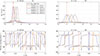Figure 6. Comparison of amplitudes (row 1) and slowly varying phases (row 2) along the point reception axis (at z = d) under no-flow, uniform and laminar flow conditions (Eqs. (8) and (4)) for a frequency of 500 kHz (ka = 78.5). Flow velocities of v avg = 8 m/s, 24 m/s and 40 m/s (column 3) when d = 0.5 (column 1) and 1 m (column 2) are applied. The red vertical dashed line (x = 0) marks the point-receiver position.

Figure 6 displays the amplitudes (row 1) and slowly varying phases (row 2) for a frequency of 500 kHz (ka = 78.5), for flow velocities of v _avg = 8 m/s, 24 m/s and 40 m/s. The two different pipe diameters d = 0.5 (column 1) and 1 m (column 2) are applied.

In line with the results mathematically shown in Section 2.3, a good agreement between the uniform and laminar flow velocity profiles is observed for both amplitude and slowly varying phase along the point receiver axis at z = d. The position of maximum sound field at z = d shifts as expected downstream as the flow velocity increases (Figs. 6a and 6b). This is explained by the tilt of the sound pressure field, as mentioned in Sections 3.2 and 3.3.

3.6 Comparison between acoustic waves under a uniform and a laminar flow profile for different pipe diameters d

The tilt and distortion of the acoustic beam due to the flow velocity profile can significantly deviate the main lobe of the sound beam from the direction of the no-flow acoustic axis as demonstrated in Sections 3.2 and 3.3. This can potentially introduce measurement errors in transit time measurements [46]. Therefore, a further investigation on the amplitude and phase of the acoustic wave in different flow velocity profiles along the no-flow acoustic axis is relevant. This is here carried out by numerical comparison of the acoustic field through a uniform and a laminar flow velocity profile along the no-flow acoustic axis up to the reception point at z = d.

Figure 7 presents a comparison of amplitudes (column 1) and slowly varying phase (column 2) at no-flow conditions and under a uniform and a laminar flow velocity profile along the no-flow acoustic axis (x = y = 0) up to the reception point at z = d = 0.5 m, for frequencies of 150 kHz (ka = 23.6, row 1) and 500 kHz (ka = 78.5, row 2). The red dot indicates the reception point at z = d = 0.5 m. The average flow velocity is 40 m/s for both flow velocity profiles.

Figure 7. Comparison of amplitudes (column 1) and slowly varying phases (column 2) through a uniform (Eq. (8)) and a laminar (Eq. (4)) flow velocity profile along the no-flow acoustic axis (x = y = 0) up to z = d = 0.5 m, for frequencies of 150 kHz (ka = 23.6, row 1) and 500 kHz (ka = 78.5, row 2). The red dot indicates the reception point at z = d. The Rayleigh distances R 1 (for 150 kHz) and R 2 (for 500 kHz) is indicated by the pink vertical dashed line. The minimal distances L 1 (for 150 kHz) and L 2 (for 500 kHz) are indicated by the red vertical dashed line. Flow velocity of v avg = 40 m/s is applied.

In Figure 7 it is seen that at z = d/2 = 0.25 m and at z = d = 0.5 m the amplitude under the uniform flow velocity is equal to the amplitude under the laminar flow profile. This is also the case for the slowly varying phase. It is in agreement with the mathematical proof in Section 2.3. In Figure 8, this is further illustrated by showing that the ray paths obtained under a uniform flow velocity profile (Eq. (16), solid line) and a laminar flow velocity profile ((14), dashed line) intersect at z = d/2 = 0.25 m and at z = d = 0.5 m. Flow velocities of v _avg = 8 m/s, 24 m/s and 40 m/s are used.

Figure 8. Comparison of ray paths under a uniform (Eq. (16), solid line) and a laminar (Eq. (14), dashed line) flow velocity profile over the propagation distance up to z = d = 0.5 m. Flow velocities of v avg = 8 m/s, 24 m/s and 40 m/s are applied.

At other distances than z = d/2 = 0.25 m and at z = d = 0.5 m, the amplitudes for the laminar and the uniform flow velocity profile cases do not overlap, as expected. The difference between the no-flow case and the two flow cases is larger for 500 kHz than for 150 kHz since the beam in the 500 kHz case is tilted so much that the second side lobe covers the no-flow axis.

Up to z = 0.2 m, a fair agreement is seen in the slowly varying phase between the no-flow and laminar flow velocity profiles at 150 kHz (Fig. 7c). Moreover, a significant gap is observed with the uniform flow velocity profile compared to the no-flow and laminar flow velocity profiles. From z = 0.25 m and beyond, a fair agreement between the slow phase for the uniform and laminar flow velocity profiles is observed. Both slowly varying phases tend towards −90°. The reason behind this is that in both cases, the main lobe of the sound field still points in the direction of the no-flow acoustic axis, as discussed above.

This is not the case at a frequency of 500 kHz (Fig. 7d). For the 500 kHz case in Figure 7d, no close agreement is seen between the different flow velocity profiles. This is mainly due to (i) the “S-shape” illustrated by the sound pressure field in the laminar flowing regime, compared to uniform flow case where the sound pressure field is straight over the acoustic path and (ii) the second side lobe of the sound field points in the direction of the no-flow acoustic axis.

Figures 9 (amplitudes) and 10 (slow varying phases) are similar to Figure 8, except that plots are displayed for the two frequencies of 150 kHz (row 1) and 500 kHz (row 2), and for flow velocities of v _avg = 8 m/s (column 1), 24 m/s (column 2) and 40 m/s (column 3), respectively. Pipe diameters of d = 0.1 m, 0.5 m, 1 m, 5 m and 10 m are used for further comparisons of the acoustic wave along the no-flow acoustic axis. Pipe diameters larger than 1 m are just applied for better visualizations of diffraction and flow effects on the sound wave well in the farfield.

Figure 9. Comparison of amplitudes through uniform (Eq. (8)) and a laminar (Eq. (4)) flow velocity profile along the no-flow acoustic axis (x = y = 0) up to z = d = 10 m, for frequencies of 150 kHz (ka = 23.6, row 1) and 500 kHz (ka = 78.5, row 2). The red dot indicates the reception point at z = d for each pipe diameter. v avg = 8 m/s (column 1), v avg = 24 m/s (column 2), and v avg = 40 m/s (column 3).

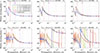Figure 10. Comparison of slowly varying phases through a uniform (Eq. (8)) and a laminar (Eq. (4)) flow velocity profile along the no-flow acoustic axis (x = y = 0) up to z = d = 10 m, for frequencies of 150 kHz (ka = 23.6, row 1) and 500 kHz (ka = 78.5, row 2). The red dot indicates the reception point at z = d for each pipe diameter. v avg = 8 m/s (column 1), v avg = 24 m/s (column 2), and v avg = 40 m/s (column 3).

In Figures 9a and 10a for the 150 kHz (row 1), a good agreement is observed between amplitudes and slowly varying phases for the flow velocity of v _avg = 8 m/s under uniform and laminar flow velocity profiles, and for different pipe diameters. This is agreement is not seen for the same flow velocity when the frequency is 500 kHz (row 2, (d)). Moreover, for flow velocities of 24 m/s and 40 m/s, no close agreement between amplitudes and slowly varying phases is observed for the two frequencies as seen in Figures 9b–9c, 9e–9f and 10b–10c, 10e–10f.

The two before-mentioned intersection points at mid-distance z = d/2 and at the reception point z = d under uniform and laminar flow velocity profiles are also observed in Figures 9 and 10 where different pipe diameters are considered.

4 Conclusion

In this work, a theoretical investigation of the sound beam through a flowing fluid has been carried out, by use of a high-frequency, narrow-angle three-dimensional parabolic equation. The sound field is generated by a uniform circular piston source located in a flat baffle at z = 0 radiating into the positive half-space. The flow is in a direction perpendicular to the main propagation direction of the flow. Part of the motivation for the work is from ultrasonic flow meters even if the geometry used here is not the same as in such meters. However, the study of acoustic beams in a flowing fluid is of general relevance for these applications.

Integral solutions have been developed for uniform flow and for a parabolic flow profile which is typical for laminar flow. Wall reflections at the opposite side from the source (z = d) have not been taken into consideration. For validation purposes, results from the integral solutions have been shown to match path calculations by ray acoustics.

A main result from this work is that, for the same average flow velocity, the acoustic field at the opposite pipe wall (z = d) is the same regardless of the flow velocity profile (uniform or laminar). This result is valid for both amplitude and phase, and for all lateral positions x and y. This observation is true also at the pipe centre (z = d/2). This is in agreement with ray acoustics, ray paths for either uniform or laminar flow profiles intersecting at these two points (z = d/2 and z = d). Even if the geometry studied in this work is not identical to the geometry in ultrasonic flow meters, this result is nevertheless important for justifying the use of simplifying uniform flow assumption in ultrasonic flow meters applications.

Sound beams have been calculated for flow velocities ranging from 0 m/s to 40 m/s, corresponding to a Mach number up to 0.1 as the speed of sound is set to 400 m/s, a typical number for natural gas. The radius of the uniform piston is selected as 1 cm. The simulations have been carried out for 150 kHz and 500 kHz. As expected, the acoustic beam will be bent more the higher the flow velocity is. For the laminar flow, this leads to an “S-shape” of the acoustic beam as the flow profile is parabolic, with low flow close to the sound source and close to the opposite pipe wall, and higher flow in-between. This “S-shape” is more easily seen at 500 kHz, as the acoustic beams is then is more narrow than the beam at 150 kHz.

The sound field along the no-flow acoustic axis (x = y = 0) has been studied more in detail. As the flow increases, the bending of the beam will affect the sound field. For large pipes, where the opposite pipe wall is in the farfield, a 1/z decay is seen at 150 kHz as the main lobe still covers the no-flow acoustic axis. At 500 kHz, the beams is more narrow. This means that the main lobe does not cover the no-flow acoustic axis for flow velocity of 16 m/s and above. Therefore, the amplitude decay is more unsteady, and not 1/z.

Similarly, the slowly varying phase at 150 kHz approaches −90° well beyond the Rayleigh distance. At 500 kHz, its approaches either −90° or +90° depending on the flow velocity. This depends on whether the main lobe, first side lobe or second side lobe covers the no-flow acoustic axis.

Finally, the results from this work illustrates that the diffraction effect depends on the path length, the ka number and also on the flow velocity, as expected. This indicates that the effect of flow on the diffraction correction should be considered for the acoustic beam used in ultrasonic flow meters.

Funding

This work was supported by the Western Norway University of Applied Sciences (HVL), Bergen, Norway.

Conflicts of interest

The authors hereby declare no conflict of interest to disclose.

Data availability statement

The research data associated with this article are included within the article.

Author contribution statement

Daudel Tchatat Ngaha: Conceptualization, Writing – original draft – review \AMP editing, Simulations, Methodology, Formal analysis. Kjell-Eivind Frøysa: Writing – review \AMP editing, Methodology, Formal analysis, Supervision, Funding acquisition.

References

Appendix A

Derivation of the integral solution

Without loss of generality, let us consider equation (2), where the components v _0x (z) and v _0y (z) of the flow velocity are initially taken into account. The aim here is to derive a general form of the integral expression that incorporates both flow velocity components simultaneously. Under this assumption, we arrive at the following equation which is given by

$$\begin{array}{cc}\hfill {\mathrm{\Delta }}_{\perp }q(X)& +\text{i}{\alpha }_1{v}_{0x}(z)\frac{\partial q(X)}{\partial x}+\text{i}{\alpha }_1{v}_{0y}(z)\frac{\partial q(X)}{\partial y}\hfill \\ \hfill & +\text{i}\alpha \frac{\partial q(X)}{\partial z}=0,\hfill \end{array}$$(A.1)

where X = (x, y, z), ${\alpha }_1=\frac{2k}{c}$, α ₂ = 2k, v _0x (z)=v _xmax(1−(z−R)²/R ²) and v _0y (z)=v _ymax(1−(z−R)²/R ²), R = d/2 is the pipe radius. The boundary condition in equation (3) can be rewritten as q(x, y, 0)=h(x, y) when x ² + y ² <  a ² (ℒ), $h(x,y)={\rho }_{0}c{\overline{v}}_s$.

By taking the two-dimensional spatial Fourier transformation in x and y coordinates in equation (A.1), with X ↦ k (so $q(X,z)\mapsto \widehat{q}(k,z)$) where k = (k ₁, k ₂), one has

$$\begin{array}{cc}\hfill -(k_1^2+k_2^2)\widehat{q}& +\text{i}{\alpha }_1[\text{i}{v}_{0x}(z)k_1+\text{i}{v}_{0y}(z)k_2]\widehat{q}\hfill \\ \hfill & +\text{i}{\alpha }_2\frac{\mathrm{d}\widehat{q}}{\mathit{dz}}=0.\hfill \end{array}$$(A.2)

This equation can be rewritten as an ordinary differential equation with respect to z as follows

$$\begin{array}{cc}& \frac{\mathrm{d}\widehat{q}(k,z)}{\widehat{q}(k,z)}\hfill \\ \hfill & =\frac{[k_1^2+k_2^2+{\alpha }_1{v}_{0x}(z)k_1+{\alpha }_1{v}_{0y}(z)k_2]}{\text{i}{\alpha }_2}\mathrm{d}z.\hfill \end{array}$$(A.3)

However, the antiderivatives of v _0x (z) and v _0y (z) with respect to z are given by

$$\begin{array}{cc}\hfill v_x^{\ast }(z)& =v_{x\text{max}}(z-\frac{{(z-R)}^3}{3R^2}),\hfill \\ \hfill v_y^{\ast }(z)& =v_{y\text{max}}(z-\frac{{(z-R)}^3}{3R^2})·\hfill \end{array}$$

With this in mind, a solution of the equation (A.3) can be written as

$$\begin{array}{c}\hfill \widehat{q}(k,z)=A(k,z)·{\text{e}}^{\frac{[(k_1^2+k_2^2)z+{\alpha }_1{v}_x^{\ast }(z)k_1+{\alpha }_1{v}_y^{\ast }(z)k_2]}{\text{i}{\alpha }_2}}·\end{array}$$(A.4)

A(k, z) is determined below by using the boundary condition at z = 0

$$\begin{array}{cc}\hfill \widehat{q}{(k,z)|}_{z=0}& =A(k){\text{e}}^{\frac{(\frac{{\alpha }_1{k}_1{v}_{x\text{max}}R}{3}+\frac{{\alpha }_1{k}_2{v}_{y\text{max}}R}{3})}{\text{i}{\alpha }_2}}\hfill \\ \hfill & =\mathcal{F}(h(x,y))=\widehat{h}(k),\hfill \end{array}$$(A.5)

then

$$\begin{array}{c}\hfill A(k)=\widehat{h}(k){\text{e}}^{-\frac{(\frac{{\alpha }_1{k}_1{v}_{x\text{max}}R}{3}+\frac{{\alpha }_1{k}_2{v}_{y\text{max}}R}{3})}{\text{i}{\alpha }_2}},\end{array}$$(A.6)

since v _x ^*(0)=v _xmax R/3 and v _y ^*(0)=v _ymax R/3.

Plugging equation (A.6) into (A.4) yields

$$\begin{array}{cc}\hfill \widehat{q}(k,z)=& =\widehat{h}(k){\text{e}}^{\frac{[(k_1^2+k_2^2)z+{\alpha }_1^{\ast }{k}_1+{\alpha }_2^{\ast }{k}_2]}{\text{i}{\alpha }_2}},\hfill \end{array}$$(A.7)

where

$$\begin{array}{c}\hfill {\alpha }_1^{\ast }={\alpha }_1(v_x^{\ast }(z)-\frac{R{v}_{x\text{max}}}{3})\end{array}$$

and

$$\begin{array}{c}\hfill {\alpha }_2^{\ast }={\alpha }_1(v_y^{\ast }(z)-\frac{R{v}_{y\text{max}}}{3})·\end{array}$$

After some algebra arrangement, equation (A.7) can be rewritten as follows

$$\begin{array}{cc}\hfill \widehat{q}(k,z)& =\widehat{h}(k){\text{e}}^{\frac{[{(k_1+\frac{\overline{{\alpha }_1}}{2})}^2+{(k_2+\frac{\overline{{\alpha }_2}}{2})}^2]z-\frac{({\overline{{\alpha }_1}}^2+{\overline{{\alpha }_2}}^2)}{4}z}{\text{i}{\alpha }_2}},\hfill \end{array}$$(A.8)

where $\overline{{\alpha }_1}=\frac{{\alpha }_1^{\ast }}{z}$ and $\overline{{\alpha }_2}=\frac{{\alpha }_2^{\ast }}{z}$.

Next, by using the 2D inverse Fourier transform in equation (A.8), one has

$$\begin{array}{cc}\hfill q(X)=& \frac{1}{{(2\pi )}^2}\int {\int }_{\mathcal{L}}\widehat{q}(k,z){\text{e}}^{\text{i}(k_{1}x+k_{2}y)}\mathrm{d}{k}_1\mathrm{d}{k}_2,\hfill \\ \hfill =& \frac{1}{{(2\pi )}^2}\int {\int }_{\mathcal{L}}\widehat{h}(k){\text{e}}^{\frac{(k_1^2+k_2^2+\overline{{\alpha }_1}{k}_1+\overline{{\alpha }_2}{k}_2)z}{\text{i}{\alpha }_2}}\hfill \\ \hfill & \times {\text{e}}^{\text{i}(k_{1}x+k_{2}y)}\mathrm{d}{k}_1\mathrm{d}{k}_2,\hfill \\ \hfill =& \frac{{\text{e}}^{-\left(\frac{{\overline{{\alpha }_1}}^2+{\overline{{\alpha }_2}}^2}{4\text{i}{\alpha }_2}\right)z}}{{(2\pi )}^2}\hfill \\ \hfill & \times \int {\int }_{\mathcal{L}}(\int {\int }_{\mathcal{L}}\frac{h(x_0,y_0)}{{(2\pi )}^2}{\text{e}}^{-\text{i}(k_1{x}_0+k_2{y}_0)}\mathrm{d}{x}_0\mathrm{d}{y}_0)\hfill \\ \hfill & \times {\text{e}}^{\frac{{(k_1+\frac{\overline{{\alpha }_1}}{2})}^2+{(k_2+\frac{\overline{{\alpha }_2}}{2})}^2}{\text{i}{\alpha }_2}z}{\text{e}}^{\text{i}(k_{1}x+k_{2}y)}\mathrm{d}{k}_1\mathrm{d}{k}_2.\hfill \end{array}$$(A.9)

After some algebra arrangement, the equation above can be rewritten as follows

$$\begin{array}{cc}\hfill q(X)& =\frac{{\text{e}}^{-\left(\frac{{\overline{{\alpha }_1}}^2+{\overline{{\alpha }_2}}^2}{4\text{i}{\alpha }_2}\right)z}}{{(2\pi )}^2}\hfill \\ \hfill & \times \{\int {\int }_{\mathcal{L}}(\frac{1}{{(2\pi )}^2}\int {\int }_{\mathcal{L}}{\text{e}}^{\text{i}[K_1(x-x_0)+K_2(y-y_0)]}\hfill \\ \hfill & ·{\text{e}}^{\frac{-\text{i}(K_1^2+K_2^2)}{\alpha }z}\mathrm{d}{K}_1\mathrm{d}{K}_2)\hfill \\ \hfill & \times h(x_0,y_0){\text{e}}^{-\text{i}[\frac{\overline{{\alpha }_1}}{2}(x-x_0)+\frac{\overline{{\alpha }_2}}{2}(y-y_0)]}\mathrm{d}{x}_0\mathrm{d}{y}_0\},\hfill \end{array}$$(A.10)

where we scaled $K_1=k_1+\frac{\overline{{\alpha }_1}}{2}$ and $K_2=k_2+\frac{\overline{{\alpha }_2}}{2}$, so dk ₁ = dK ₁ and dk ₂ = dK ₂. Indeed, if we set $\phi (k_1,k_2)=(K_1-\frac{\overline{{\alpha }_1}}{2},K_2-\frac{\overline{{\alpha }_2}}{2})$, then dk ₁dk ₂ = det|φ(k ₁, k ₂)| × dK ₁dK ₂ = 1 × dK ₁dK ₂. Thus, one will get

$$\begin{array}{cc}\hfill q(X)& =\frac{{\text{e}}^{-\left(\frac{{\overline{{\alpha }_1}}^2+{\overline{{\alpha }_2}}^2}{4\text{i}{\alpha }_2}\right)z}}{{(2\pi )}^2}\int {\int }_{\mathcal{L}}{\mathcal{F}}^{-1}\left[{\text{e}}^{\frac{-\text{i}(K_1^2+K_2^2)}{{\alpha }_2}z}\right]\hfill \\ \hfill & \times {\text{e}}^{-\text{i}[\frac{\overline{{\alpha }_1}}{2}(x-x_0)+\frac{\overline{{\alpha }_2}}{2}(y-y_0)]}h(x_0,y_0)\mathrm{d}{x}_0\mathrm{d}{y}_0.\hfill \end{array}$$(A.11)

As a Fourier transform of a Gaussian is a Gaussian and the inverse Fourier transform of a Gaussian is a Gaussian, then in 2D, one has

$$\begin{array}{c}\hfill {\mathcal{F}}^{-1}\left[{\text{e}}^{\frac{-\text{i}(K_1^2+K_2^2)}{{\alpha }_2}z}\right]=\frac{\pi {\alpha }_2}{\text{i}z}{\text{e}}^{\frac{-{\alpha }_2({(x-x_0)}^2+{(y-y_0)}^2)}{4\text{i}z}}.\end{array}$$(A.12)

Thus, equation (A.11) can be rewritten as

$$\begin{array}{cc}\hfill q(X)& =\frac{\pi {\alpha }_2{\text{e}}^{-\left(\frac{{\overline{{\alpha }_1}}^2+{\overline{{\alpha }_2}}^2}{4\text{i}{\alpha }_2}\right)z}}{4\text{i}z{\pi }^2}\int {\int }_{\mathcal{L}}\{{\text{e}}^{\frac{-{\alpha }_2({(x-x_0)}^2+{(y-y_0)}^2)}{4\text{i}z}}\hfill \\ \hfill & \times {\text{e}}^{-\text{i}[\frac{\overline{{\alpha }_1}}{2}(x-x_0)+\frac{\overline{{\alpha }_2}}{2}(y-y_0)]}h(x_0,y_0)\}\mathrm{d}{x}_0\mathrm{d}{y}_0.\hfill \end{array}$$(A.13)

This leads to the following integral solution of equation (A.8) given by

$$\begin{array}{cc}& q(X)=\frac{\pi {\alpha }_2{\text{e}}^{-\left(\frac{{\overline{{\alpha }_1}}^2+{\overline{{\alpha }_2}}^2}{4\text{i}{\alpha }_2}\right)z}}{4\text{i}z{\pi }^2}\int {\int }_{\mathcal{L}}\{{\text{e}}^{\frac{-{\alpha }_2({(x-x_0)}^2+{(y-y_0)}^2)}{4\text{i}z}}\hfill \\ \hfill & \times {\text{e}}^{-\text{i}[\frac{\overline{{\alpha }_1}}{2}(x-x_0)+\frac{\overline{{\alpha }_2}}{2}(y-y_0)]}h(x_0,y_0)\}\mathrm{d}{x}_0\mathrm{d}{y}_0.\hfill \end{array}$$(A.14)

Since

$$\begin{array}{cc}& -\left(\frac{{\overline{{\alpha }_1}}^2+{\overline{{\alpha }_2}}^2}{4\text{i}{\alpha }_2}\right)z=\frac{\text{i}k}{2z{c}^2}\{{(v_x^{\ast }(z)-\frac{R{v}_{x\text{max}}}{3})}^2\hfill \\ \hfill & +{(v_y^{\ast }(z)-\frac{R{v}_{y\text{max}}}{3})}^2\},{\alpha }_2=2k,\hfill \\ \hfill & \frac{\overline{{\alpha }_1}}{2}=\frac{k}{\mathit{zc}}(v_x^{\ast }(z)-\frac{R{v}_{x\text{max}}}{3})\text{and}\hfill \\ \hfill & \frac{\overline{{\alpha }_2}}{2}=\frac{k}{\mathit{zc}}(v_y^{\ast }(z)-\frac{R{v}_{y\text{max}}}{3}),\hfill \end{array}$$

plugging these elements above and h into equation (A.14) yields

$$\begin{array}{cc}\hfill q(X)=& \frac{k{\rho }_{0}c{\text{e}}^{\frac{\text{i}k[{(v_x^{\ast }(z)-\frac{R{v}_{x\text{max}}}{3})}^2+{(v_y^{\ast }(z)-\frac{R{v}_{y\text{max}}}{3})}^2]}{2z{c}^2}}}{2\text{i}\pi z}\hfill \\ \hfill & \times \int {\int }_{\mathcal{L}}\{{\text{e}}^{\frac{\text{i}k({(x-x_0)}^2+{(y-y_0)}^2)}{2z}}\hfill \\ \hfill & \times {\text{e}}^{\frac{-\text{i}k[(v_x^{\ast }(z)-\frac{R{v}_{x\text{max}}}{3})(x-x_0)+(v_y^{\ast }(z)-\frac{R{v}_{y\text{max}}}{3})(y-y_0)]}{\mathit{zc}}}\hfill \\ \hfill & \times {\overline{v}}_s(x_0,y_0)\}\mathrm{d}{x}_0\mathrm{d}{y}_0.\hfill \end{array}$$(A.15)

Since we consider fluid flow only in the x-direction, equation (A.15) reduces to

$$\begin{array}{cc}\hfill q(X)=& \frac{k{\rho }_{0}c}{2\text{i}\pi z}{\text{e}}^{\stackrel{A_1}{\overbrace{\frac{\text{i}k}{2z{c}^2}{(v_x^{\ast }(z)-\frac{R{v}_{\text{max}}}{3})}^2}}}\hfill \\ \hfill & \times \int {\int }_{\mathcal{L}}{\text{e}}^{\frac{\text{i}k({(x-x_0)}^2+{(y-y_0)}^2)}{2z}}\hfill \\ \hfill & \times {\text{e}}^{\stackrel{B_1}{\overbrace{\frac{-\text{i}k}{\mathit{zc}}(v_x^{\ast }(z)-\frac{R{v}_{\text{max}}}{3})(x-x_0)}}}\hfill \\ \hfill & \times {\overline{v}}_s(x_0,y_0)\mathrm{d}{x}_0\mathrm{d}{y}_0,\hfill \end{array}$$(A.16)

with the maximum flow velocity $v_{\text{max}}=v_{x\text{max}}=\frac{3}{2}{v}_{\text{avg}}$.

Let us simplify the expressions A ₁ and B ₁ in equation (A.16)

$$\begin{array}{c}\hfill A_1=\text{i}kz\frac{v_{\text{avg}}^2}{2c^2}{\left(\frac{z}{2R}\right)}^2{(3-\frac{z}{R})}^2\end{array}$$

and

$$\begin{array}{c}\hfill B_1=\frac{-\text{i}k}{c}{v}_{\text{avg}}\frac{z}{2R}[3-\frac{z}{R}](x-x_0).\end{array}$$

Plugging A ₁ and B ₁ into equation (A.16) yields

$$\begin{array}{cc}& q(x,y,z)=\frac{k{\rho }_{0}c}{2\text{i}\pi z}{\text{e}}^{\text{i}kz\frac{M^2}{2}{\left(\frac{z}{2R}\right)}^2{(3-\frac{z}{R})}^2}\hfill \\ \hfill & \times \int {\int }_{\mathcal{L}}\{{\text{e}}^{\frac{\text{i}k({(x-x_0)}^2+{(y-y_0)}^2)}{2z}}\hfill \\ \hfill & \times {\text{e}}^{-\text{i}kM\left(\frac{z}{2R}\right)(3-\frac{z}{R})(x-x_0)}{\overline{v}}_s(x_0,y_0)\}\mathrm{d}{x}_0\mathrm{d}{y}_0,\hfill \end{array}$$(A.17)

with $M=\frac{v_{\text{avg}}}{c}$ is the flow Mach number. This completes the proof.

Appendix B

Stationary phase approximation

In this appendix, two additional methods to determine the path followed by the maximal sound field by use of the integral solution equation (4) are presented.

Option 1:

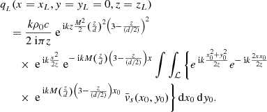
The approach of this method is to consider the maximal amplitude of the sound field pressure which mostly relies on the integrand of equation (B.1) below as this includes the integrand peaks due to source orientation and where beam patterns are more directional.

$$\begin{array}{cc}& q_{{}_L}(x=x_L,y=y_L=0,z=z_L)\hfill \\ \hfill & =\frac{k{\rho }_{0}c}{2\text{i}\pi z}{\text{e}}^{\text{i}kz\frac{M^2}{2}{\left(\frac{z}{d}\right)}^2{(3-\frac{z}{(d/2)})}^2}\hfill \\ \hfill & \times {\text{e}}^{\text{i}k\frac{x^2}{2z}}{\text{e}}^{-\text{i}kM\left(\frac{z}{d}\right)(3-\frac{z}{(d/2)})x}\int {\int }_{\mathcal{L}}\{e^{\text{i}k\frac{x_0^2+y_0^2}{2z}}{e}^{-\text{i}k\frac{2x{x}_0}{2z}}\hfill \\ \hfill & \times {\text{e}}^{\text{i}kM\left(\frac{z}{d}\right)(3-\frac{z}{(d/2)})x_0}{\overline{v}}_s(x_0,y_0)\}\mathrm{d}{x}_0\mathrm{d}{y}_0.\hfill \end{array}$$(B.1)

With this in mind, it is possible to determine the path followed by this maximum, which in our case is the dominant propagation direction of the sound pressure field. This is done by identifying terms where the phase of the integrand changes slowly. These terms, contribute most to the integral. Thus, by taking out the rapidly varying phase which is the second-order component (first exponential terms) in the integrand equation (B.1), and keeping only the first-order components, the dominant propagation direction x _L can be determined using the phase from the exponential terms in the integrand (B.1) given by

$$\begin{array}{c}\hfill -\text{i}k\frac{2x_L{x}_0}{2z}+\text{i}kM\left(\frac{z_L}{d}\right)(3-\frac{z_L}{(d/2)})x_0=0.\end{array}$$(B.2)

After some algebra arrangement, it leads to

$$\begin{array}{c}\hfill x_L=\frac{3}{2}\frac{v_{\text{avg}}}{c}{z}_L[-\frac{4}{3}{\left(\frac{z_L}{d}\right)}^2+\frac{2z_L}{d}]·\end{array}$$(B.3)

Equation (B.3) is identical to equation (14). The method applied here is similar to the stationary phase approximation as we simply isolate the rapidly varying phase in the integrand. This then introduces the next option.

Option 2:

The stationary phase approximation [47–49] can allow to isolating the dominant direction of propagation, often corresponding to the path of the main lobe of the sound pressure field. Note that this method gives a clear, analytical prediction of the dominant acoustic path or trajectory of the sound field. To apply this method, we first isolate the phase from the exponential terms in the integrand in equation (B.1) written as

$$\begin{array}{c}\hfill \varphi =\text{i}k\frac{x_0^2+y_0^2}{2z}-\text{i}k\frac{2x{x}_0}{2z}+\text{i}kM\left(\frac{z}{d}\right)(3-\frac{z}{(d/2)})x_0.\end{array}$$(B.4)

In order to find the stationary phase point (x ₀, y ₀) where the gradient vanishes, one has

$$\begin{array}{c}\hfill \frac{\partial \varphi }{\partial x_0}=0\text{and}\frac{\partial \varphi }{\partial y_0}=0.\end{array}$$(B.5)

The first equation in (B.5) gives

$$\begin{array}{cc}\hfill x& =x_0+M\left(\frac{z}{d}\right)(3-\frac{z}{(d/2)})z,\hfill \\ \hfill & =x_0+Mz[3\left(\frac{z}{d}\right)-2{\left(\frac{z}{d}\right)}^2],\hfill \\ \hfill & =x_0+Mz\frac{3}{2}[2\left(\frac{z}{d}\right)-\frac{4}{3}{\left(\frac{z}{d}\right)}^2].\hfill \end{array}$$

This leads to the stationary phase point (x ₀, y ₀)

$$\begin{array}{cc}\hfill y_0& =y_L=0\text{and}\hfill \\ \hfill x_L& =x_0+\frac{3}{2}\frac{v_{\text{avg}}}{c}{z}_L[-\frac{4}{3}{\left(\frac{z_L}{d}\right)}^2+\frac{2z_L}{d}]·\hfill \end{array}$$(B.6)

Thus, this means that the beam is bent sideways due to the flow, with the bending described by equation (B.6). Interestingly, equation (B.6) allows to identify the dominant trajectories contributing to the pressure sound field from each source point (x ₀, y ₀) on the uniform circular piston.

Therefore, to find the path of the main lobe of the sound pressure field, we assume that the dominant contribution comes from the center of the piston (at x ₀ = 0). Then, equation (B.6) reduces to

$$\begin{array}{c}\hfill x_L=\frac{3}{2}\frac{v_{\text{avg}}}{c}{z}_L[-\frac{4}{3}{\left(\frac{z_L}{d}\right)}^2+\frac{2z_L}{d}]·\end{array}$$(B.7)

This equation is identical to equations (14) and (B.3).

All Figures

	Figure 1. Sketch of the geometric used in this paper.
In the text

	Figure 2. Sound pressure field ($|q_{{}_L}|/\left({\rho }_{0}c{\overline{v}}_s\right)$) at no-flow conditions (v avg = 0 m/s) when (a) f = 150 kHz (ka = 23.6) and (b) f = 500 kHz (ka = 78.5) The no-flow acoustic axis and the dominant acoustic path of the sound field (Eqs. (14) and (16)) are indicated by the red and white vertical dashed lines, respectively.
In the text

Figure 3. Normalized sound pressure field under uniform ($|q_{{}_C}|/\left({\rho }_{0}c{\overline{v}}_s\right)$ [Eq. (8)], left) and laminar ($|q_{{}_L}|/\left({\rho }_{0}c{\overline{v}}_s\right)$ [Eq. (4)], right) flow velocity profiles when f = 150 kHz (ka = 23.6) and d = 0.5 m. The no-flow acoustic axis and the dominant acoustic path of the sound field (Eqs. (14) and (16)) are indicated by the red vertical and white dashed lines, respectively. v avg = 8 m/s (row 1), v avg = 24 m/s (row 2), and v avg = 40 m/s (row 3).

In the text

Figure 4. Normalized sound pressure field under uniform ($|q_{{}_C}|/\left({\rho }_{0}c{\overline{v}}_s\right)$ [Eq. (8)], left) and laminar ($|q_{{}_L}|/\left({\rho }_{0}c{\overline{v}}_s\right)$ [Eq. (4)], right) flow velocity profiles when f = 500 kHz (ka = 78.5) and d = 0.5 m. The no-flow acoustic axis and the dominant acoustic path of the sound field (Eqs. (14) and (16)) are indicated by the red vertical and white dashed lines, respectively. v avg = 8 m/s (row 1), v avg = 24 m/s (row 2), and v avg = 40 m/s (row 3).

In the text

	Figure 5. Amplitude (row 1) and slowly varying phase (row 2) along the acoustic axis at x = y = 0 for different average flow velocities under a laminar flow profile when f = 150 kHz (ka = 23.6, column 1) and f = 500 kHz (ka = 78.5, column 2).
In the text

References

- K. Attenborough: Sound Propagation in the Atmosphere, in: T. Rossing (Eds). Springer Handbook of Acoustics. Springer Handbooks. Springer, New York, NY, 2007. DOI: https://doi.org/10.1007/978-0-387-30425-0_4. [Google Scholar]
- H. Bommidala, J. Colas, A. Emmanuelli, D. Dragna, C. Khodr, B. Cotte, R.J.A.M. Stevens: Three-dimensional effects of the wake on wind turbine sound propagation using parabolic equation. Journal of Sound and Vibration 608 (2025) 119036. [Google Scholar]
- C. Erbe, A. Duncan, K.J. Vigness-Raposa: Introduction to sound propagation under water, in: C. Erbe, J.A. Thomas (Eds). Exploring Animal Behavior Through Sound: Volume 1. Springer, Cham, 2022. DOI: https://doi.org/10.1007/978-3-030-97540-1_6. [Google Scholar]
- G. Rajita, N. Mandal: Review on transit time ultrasonic flowmeter, in: 2nd International Conference on Control, Instrumentation, Energy & Communication (CIEC), Kolkata, India, 2016, pp. 88–92. https://ieeexplore.ieee.org/document/7513740. [Google Scholar]
- T.J. Hajenko, C.R. Benson: The high frequency underwater acoustic channel, in: OCEANS’10 IEEE SYDNEY, Sydney, NSW, Australia, 2010, pp. 1–3. https://ieeexplore.ieee.org/abstract/document/5603801. [Google Scholar]
- A.P. Sarvazyan, M.W. Urban, J.F. Greenleaf: Acoustic waves in medical imaging and diagnostics. Ultrasound in Medicine & Biology 39, 7 (2013) 1133–1146. https://www.sciencedirect.com/science/article/pii/S0301562913000793. [Google Scholar]
- L.C. Lynnworth, Y. Liu: Ultrasonic flowmeters: half-century progress report, Half-century progress report, 1955-2005, Ultrasonics 44, 2006, pp. 1371–1378. [Google Scholar]
- ISO International Standard 17089-2: Measurement of fluid flow in closed conduits-Ultrasonic flow meters for gas-Part 2: Meters for industrial applications, 1st edn., 2012. [Google Scholar]
- ISO International Standard 17089-1: Measurement of fluid flow in closed conduits-Ultrasonic flow meters for gas-Part 1: meters for custody transfer and allocation measurement, 2nd edn., 2019. [Google Scholar]
- Prepared for the future: Ultrasonic flow measurements in flare installations. https://www.endress.com/en/support-overview/learning-center/ultrasonic-flare#toc10 (accessed on 27/08/2025). [Google Scholar]
- Z. Wei, X. Zhao, L. Han, N. Zhao, L. Fang: Ultrasonic probes and echo time algorithms in ultrasonic gas flow measurement systems: progress and perspectives. Physics of Fluids 1, 37 (2025) 011–305. [Google Scholar]
- G. Chen, G. Liu, B. Zhu, W. Tan: 3D isosceles triangular ultrasonic path of transit-time ultrasonic flowmeter: theoretical design and CFD simulations. IEEE Sensors Journal 15 (2015) 4733–4742. [Google Scholar]
- S.F. Mousavi, S.H. Hashemabadi, J. Jamali: Calculation of geometric flow profile correction factor for ultrasonic flow meter using semi-3d simulation technique. Ultrasonics 106 (2020) 106165. [Google Scholar]
- C.D. Reid: Some investigations into the velocity of sound at ultra-sonic frequencies using quartz oscillators. Physical Review 35 (1930) 814–831. [Google Scholar]
- C.D. Reid: Notes on the effect of distance from the source on the velocity of sound at ultrasonic frequencies. Physical Review 37 (1931) 1147–1148. [Google Scholar]
- H. Seki, A. Granato, R. Truell: Diffraction effects in the ultrasonic field of a piston source and their importance in the accurate measurement of attenuation. Journal of the Acoustical Society of America 28, 2 (1956) 230–238. [Google Scholar]
- A.O. Williams Jr., The piston source at high frequencies. Journal of the Acoustical Society of America 23, 1 (1951) 1–6. [Google Scholar]
- A.S. Khimunin: Numerical calculation of the diffraction corrections for the precise measurement of ultrasonic absorption. Acustica 27, 4 (1972) 173–181. [Google Scholar]
- A.S. Khimunin: Numerical calculation of the diffraction corrections for the precise measurement of ultrasound phase velocity. Acustica 32 (1975) 192–200. [Google Scholar]
- P. Lunde, K.E. Frøysa, R.A. Kippersund, M. Vestrheim: Transient diffraction effects in ultrasonic meters for volumetric, mass and energy flow measurement of natural gas, in: Proceedings of the 21st International North sea flow Measurement Workshop, Tønsberg, Norway, October 28–31, 2003. [Google Scholar]
- P. Lunde, R.A. Kippersund, M. Vestrheim, K.E. Frøysa: Transient diffraction effects in piezo-electric ultrasonic transducers using finite element modelling, in: Proceedings of the 27th Scandinavian Symposium on Physical Acoustics, Ustaoset, Norway, January 25–28, 2004. [Google Scholar]
- E. Storheim: Diffraction effects in the ultrasonic field of transmitting and receiving circular piezoceramic disks in radial mode vibration. FE modelling and comparison with measurements in air, Bergen, Norway. Ph.D. thesis, Department of Physics and Technology, University of Bergen, 2015. [Google Scholar]
- E.N. Mosland, E. Storheim, P. Lunde, M. Vestrheim, J. Kocbach: Diffraction correction for precision measurements of sound velocity in gas. Is full receiver modelling needed? in: Proceedings of the 44th Scandinavian Symposium on Physical Acoustics, Online, Norway, February 1–2, 2021. [Google Scholar]
- A. Lygre, M. Vestrheim, P. Lunde, V. Berge: Numerical simulation of ultrasonic flowmeters, in: Proceedings of the Ultrasonics International 1987 (UI’87), London, Butterworth Scientific Ltd., Guildford, UK, July 6–9, 1987. [Google Scholar]
- M. Bezdek: A boundary integral method for modeling sound waves in moving media and its application to ultrasonic flowmeters. Ph.D. thesis, Universität Erlangen- Nürnberg, Erlangen, 2006. [Google Scholar]
- M. Bezdek, H. Landes, A. Rieder, R. Lerch: A coupled finite-element, boundaryintegral method for simulating ultrasonic flowmeters. IEEE Transactions on Ultrasonics, Ferroelectrics, and Frequency Control 54, 3 (2007) 636–646. [Google Scholar]
- M. Bezdek, A. Rieder, T. Landes, H. Struntz, R. Lerch: Numerical analysis of wave propagation in an ultrasonic flowmeter, in: Proceedings of the First Congress of Alps Adria Acoustics Association, Portoroz, Slovenia, 1–2 September 2003, pp. 573–580. [Google Scholar]
- A. Luca, K. Fodil, A. Zerarka: Full-wave numerical simulation of ultrasonic transit-time gas flowmeters, in: 2016 IEEE International Ultrasonics Symposium (IUS), Tours, France, September 2016. [Google Scholar]
- M. Simurda, L. Duggen, N.T. Basse, B. Lassen: Fourier collocation approach with mesh refinement method for simulating transit-time ultrasonic flowmeters under multiphase flow conditions. IEEE Transactions on Ultrasonics, Ferroelectrics, and Frequency Control 65, 2 (2018) 244–257. [Google Scholar]
- K.-E. Frøysa, P. Lunde, M. Vestrheim: A ray theory approach to investigate the influence of flow velocity profiles on transit times in ultrasonic flow meters for gas and liquid, in: 19th International North Sea Flow Measurement Workshop, Kristiansand, Norway, October 22–25, 2001. [Google Scholar]
- V.E. Ostashev, D.K. Wilson: Acoustics in Moving Inhomogeneous Media, 2nd edn., CRC Press 2015. [Google Scholar]
- A.D. Pierce: Wave equation for sound in fluids with unsteady inhomogeneous flow. Journal of the Acoustical Society of America 87, 6 (1990) 2292–2299. [Google Scholar]
- A.D. Pierce: Acoustics: An Introduction to Its Physical Principles and Applications. Acoustical Society of America, New York, USA, 1991. [Google Scholar]
- P. Drazin, N. Riley: The Navier–Stokes Equations: A Classification of Flows and Exact Solutions (London Mathematical Society Lecture Note Series). Cambridge University Press, Cambridge, 2006. DOI: https://doi.org/10.1017/CBO9780511526459. [Google Scholar]
- D.T. Ngaha, K.-E. Frøysa: Parabolic equation simulation of diffraction effects in a sound beam propagating through a flowing fluid. Proceedings of the Meetings on Acoustics 51, 1 (2023) 045006. [Google Scholar]
- J.N. Tjøtta, S. Tjøtta: An analytical model for the nearfield of a baffled piston transducer. The Journal of the Acoustical Society of America 68 (1980) 334–339. [Google Scholar]
- V.E. Ostashev, D.K. Wilson, M.B. Muhlestein: Wave and extra-wide-angle parabolic equations for sound propagation in a moving atmosphere. The Journal of the Acoustical Society of America 147, 6 (2020) 3969–3984. [CrossRef] [PubMed] [Google Scholar]
- V.E. Ostashev, J. Colas, D. Dragna, D.K. Wilson: Phase-preserving narrow-and wide-angle parabolic equations for sound propagation in moving media. The Journal of the Acoustical Society of America 155, 2 (2024) 1086–1102. [Google Scholar]
- F.J. Weber, Jr.: Ultrasonic beam propagation in turbulent flow. Ph.D. dissertation, Worcester Polytechnic Institute, December 16, 2003. https://www.researchgate.net/publication/241427078_Ultrasonic_Beam_Propagation_in_Turbulent_Flow. [Google Scholar]
- D. Tchatat, K.-E. Frøysa: Parabolic equation simulation of a sound beam propagating through a flowing fluid, in: Proceedings of the 45th Scandinavian Symposium on Physical Acoustics, Online, Norway, Feburary 31–January 01, 2022. [Google Scholar]
- J. Lighthill: Waves in Fluids. Cambridge University Press, 1978. [Google Scholar]
- Fluenta, Flare gas flowmeter. https://fluenta.com/wp-content/uploads/2023/09/Fluenta-FGM-160-Product-Data-Sheet.pdf (accessed on 21/02/2025). [Google Scholar]
- TechnipFMC: FMC MPU1200 ultrasonic gas flowmeter. https://info.smithmeter.com/literature/docs/ssks009.pdf (accessed on 21/02/2025). [Google Scholar]
- Q. Sonic Max: Multi-path ultrasonic gas meter with highest industry standard for custody transfer measurement. https://prod-edam.honeywell.com/content/dam/honeywell-edam/pmt/hps/products/pmc/gas/transmission/ultrasonic-meters/q-sonic-max/pmt-hps-hps-dts-q-sonic-max-metric-2401.pdf?download=false (accessed on 21/02/2025). [Google Scholar]
- J.P. Smith, J. Clancy: Calculating the speed of sound in natural gas – AGA report No. 10 to AGA report No. 8. https://asgmt.com/wp-content/uploads/2023/09/2023_Speed_of_Sound_in_Natural_Gas_From_AGA_10_to_AGA_8.pdf From November 13, 2024 (accessed on 21/02/2025). [Google Scholar]
- H. Zhang, C. Guo, J. Lin: Effects of velocity profiles on measuring accuracy of transit-time ultrasonic flowmeter. Applied Sciences 9, 8 (2019) 1648. [Google Scholar]
- V. Guillemin, S. Sternberg: Geometric Asymptotics. American Mathematical Society, 1990. [Google Scholar]
- N. Bleistein, R. Handelsman: Asymptotic Expansions of Integrals. Dover Publications, 1986. [Google Scholar]
- R. Ali, T. Dietzen, M. Scerbo, L. Vinceslas, T. Van Waterschoot, E. De Sena: Relating wave-based and geometric acoustics using a stationary phase approximation approximation of the boundary integral equation, in: Proceedings of the 10th Convention of the European Acoustics Association Forum Acusticum, 2023, pp. 3841–3847. https://dael.euracoustics.org/confs/fa2023/data/articles/001143.pdf. [Google Scholar]