| Issue |
Acta Acust.
Volume 6, 2022
|
|
|---|---|---|
| Article Number | 13 | |
| Number of page(s) | 15 | |
| Section | Atmospheric Sound | |
| DOI | https://doi.org/10.1051/aacus/2022005 | |
| Published online | 12 April 2022 | |
Scientific Article
S-shaped dependence of the sound pressure level in outdoor propagation on the effective sound speed gradient
1
TGM – Institute of Technology, Department for Research and Testing, Wexstrasse 19-23, 1200 Wien, Austria
2
University of Natural Resources and Life Sciences Vienna (BOKU), Institute of Meteorology (BOKU-Met), Gregor Mendel-Haus, Gregor-Mendel-Strasse 33, 1180 Wien, Austria
3
Kirisits Consulting Engineers, Kolpinggasse 10, 7423 Pinkafeld, Austria
4
Medical University of Vienna, Department of Radiation Oncology, Waehringer Guertel 18–20, 1090 Wien, Austria
* Corresponding author: This email address is being protected from spambots. You need JavaScript enabled to view it.
Received:
17
January
2021
Accepted:
8
February
2022
Abstract
The effective sound speed gradient is used to describe the meteorological conditions during sound measurements at roads and railways. Meteorological parameters were assessed up to a height of 10 m. The sound level differences between a reference point close to the passing vehicles and at distances of 100–500 m from motorways and railway tracks were determined. These differences were found to correlate well with the effective sound speed gradient determined from the measured temperature and wind speed gradients which follow the day/night cycle as a result of the reversing air temperature gradient, incoming solar radiation and wind conditions. The correlation with sound level differences can be approximated by an S-shaped function which is constant for large positive or negative gradients of the effective sound speed. These threshold values are a consequence of the local meteorological and attenuation conditions. The analysis shows that large effective sound speed gradients are mainly a result of the wind conditions whereas gradients without a substantial wind speed contribution are low and a result of the temperature gradient. In the distance range between 150 m and 250 m, the meteorological influences cause a level increase of 3–4 dB(A) for downward refracted sound rays (favourable sound propagation) compared to a situation without meteorological influence (effective sound speed gradient of zero). In the same distance range, meteorological conditions cause a maximum sound level attenuation of 5–10 dB(A) for upward curved sound rays (unfavourable sound propagation).
Key words: Sound propagation / Meteorology / Effective sound speed gradient / S-shaped sound level attenuation
© The Author(s), Published by EDP Sciences, 2022
 This is an Open Access article distributed under the terms of the Creative Commons Attribution License (https://creativecommons.org/licenses/by/4.0), which permits unrestricted use, distribution, and reproduction in any medium, provided the original work is properly cited.
1 Introduction
Reproducible noise measurements and standardised calculations of noise indices should be linked to clearly defined meteorological conditions which influence sound propagation conditions. This paper focusses on sound sources close to ground, in particular from road and railway traffic, and on the A-weighted sound levels which are mainly used to assess annoyance and health effects.
In such cases the relevant sound propagation takes place in the lowest part of the atmospheric boundary layer (surface layer 50–100 m during the day, and lower at night) [1]. The speed of sound and wind in the sound propagation direction are combined to derive the effective speed of sound [2, 3]. The temorary highly variable temperature (∆T/∆z) and wind speed gradients (∆u/∆z) together with wind direction (see Sect. 2.2) are combined in the effective sound speed gradient which is used to describe the meteorological influence for sound propagation with one single number. The positive radiation balance present during daytime usually results in a strong temperature decrease with height, and thus, an unstable thermal layering (negative temperature gradient). At night with a clear sky, a negative radiation balance results in a strong cooling of the ground which leads to a temperature increase with height and therefore to stable layering (positive temperature gradient – inversion).
Below, a few examples can be found where acoustic with meteorological measurements are correlated. Heimann and Salomons [4] correlated the long-term sound level and meteorological measurements on a 50 m high tower. Using sound speed profiles (log-linear relationship), 121 representative meteorological situations were defined for which the sound levels were calculated with the parabolic equation. Hard and absorbing ground was assumed and the changes in the sound levels up to 1000 m distance from the sound source were calculated. As a result of the changing meteorological conditions, the sound levels changed by 9 dB at a distance of 200 m and by 21 dB at a distance of 1000 m from the sound source over absorbing ground. Sound propagation calculations with various computer programs and codes are shown in Salomons [3] while theoretical aspects of sound propagation are discussed by Ostashev and Wilson [5].
Measured effects of the atmospheric boundary layer on the sound propagation determined during the period from the early evening to the next day are presented by Hohenwarter and Mursch-Radlgruber [6] and Attenborough and van Renterghem [2] (Sect. 1.4.3). In particular, the measured height-dependent temperature and wind speed distributions are compared with the results of log-linear profiles as they are also commonly used for sound propagation calculations.
In Hohenwarter and Jelinek [7] and [8] for example, Snell`s Law of refraction is derived for a moving stratified medium with different temperatures and different wind speeds in each layer. The difference between the improved refraction law and the usual approximation [9] was found to be small.
The main idea of Salomons and Bakri [10] is to describe the meteorological influence on sound propagation with an empirical S-shaped function describing the effective sound speed gradient, and this will be discussed and applied to our measurement data.
They show results of calculations with Harmonoise and a PE Model for a logarithmic-linear sound speed profile that the sound level attenuation as a function of the effective wind speed (which corresponds to the effective sound speed gradient, see Sect. 4) follows an S-shaped curve. From a mathematical point of view, the density function of the normal distribution is a bell curve. The cumulative distribution function of the normal distribution follows a sigmoid (S-shaped) curve. The calculations are done for upward and downward refraction conditions and show that the sound level attenuation is dependent on the effective wind speed and which is constant for large values of the effective wind speed dependent on the geometrical conditions (distance and receiver height). The results of these calculations [10] are compared with our measurements.
2 Measurements at different locations and calculation of the effective sound speed gradient
2.1 Measurement set-up
In all cases, meteorological measurements were carried out with a tower of at least 10 m, where the wind speed and direction together with the air temperature were recorded continuously at different heights (temperature at 0.3 m, 2 m, 5 m, and 10 m, wind speed and direction at 2 m, 5 m, and 10 m). The 2 m and 10 m levels were used to calculate the sound speed gradient.
Temperature was measured with a 0.2 mm K-type thermocouple in passive radiation shield while a 2-dimensional sonic anemometer (Decagon DS2) was used for wind speed and direction. Humidity (Campbell Scientific CS215 in passive radiation shield), net radiation (Schenk 8111 at Markt Allhau and Aderklaa as well as Kipp & Zonen NR-Light at Bad Voeslau) and global radiation (Schenk 8102) were measured at a height of 2 m. For data collection, a Campbell Scientific CR1000 datalogger averaging for 10 min (sampling interval of 10 s) was used and Decagon DS2 data was collected at 10-min intervals.
The acoustic measurements were performed with a ½″ microphone type G.R.A.S. 40AE with preamplifier 26CA/26AK, an analysis unit type Sinus Soundbook_light with software Samurai 1.7.10, Sinus Soundbook_octav with software Samurai 1.7.14 and three Sound Analyser Nor140 (Norsonic). Brüel & Kjaer 4231 and 4230 calibrators were used for calibration.
Measurements at roads were carried out in 5-min (Bad Voeslau) or 10-min (Markt Allhau) intervals for A-weighted equivalent continuous sound pressure level LA,eq [11] differences (∆LA,eq) to correlate with the corresponding meteorological data. At the railway tracks (Aderklaa), the sound exposure level LA,E [11] differences (∆LA,E) for each individual train passing were correlated.
Those differences (∆LA,eq and ∆LA,E) were always referred to the reference point nearby the passing vehicles. It was generally ensured that each pass-by had to exceed the ambient noise by at least 8 dB(A) to be included in the analysis. Wind direction was defined with respect to the line perpendicular to almost straight-line sound sources in the experiments.
2.2 Calculation of the effective sound speed gradient
To simplify the complex behaviour of the inhomogeneous atmosphere, a stratified atmosphere can be assumed. This allows the laws of refraction to be applied when other effects such as turbulence are excluded.
To combine the effect of the temperature and wind velocity, the effective sound speed is introduced [2–4]. The effective sound speed is the sum of the height dependent speed of sound c(z) and the component of the horizontal wind speed u(z) between source and receiver. The angle α is between the source-receiver path and the wind vector:
 (1)
(1)
The refraction of the sound ray is determined primarily by the gradient of the effective sound speed [12, 13]. As a result of the ray acoustics there is a correlation between the refraction of the sound ray and the measured sound level. Gradients dceff/dz < 0 result in upward refraction of the sound rays and a decrease of the sound level, whereas dceff/dz > 0 results in downward refraction and an increase of the sound level. The sound speed in air is calculated using  where κ = cp/cv is the ratio of the specific heats for constant pressure cp and constant volume cv, R is the gas constant (R = 287 J/kg K for dry air) and T(z) is the temperature measured in Kelvin.
With the first term of the Taylor series expressed as finite differences ![Mathematical equation: $ c={c}_0\left[1+0.5\left(\Delta T/{T}_0\right)\right]$](/articles/aacus/full_html/2022/01/aacus210007/aacus210007-eq3.gif) it results in the effective sound speed gradient
it results in the effective sound speed gradient  ,
,
 (2)
(2)
The temperature gradient T′ is calculated from the measured temperature difference T′ = (T10m − T2m)/Δz and the wind gradient u′ = (u10m − u2m)/Δz, where ∆z = 8 m. Temperature and wind profiles are normally not linear, but can be linearly approximated close to the surface (see Figs. 4 and 5 of [6] and Fig. 1.14 of [2]).
The effective sound speed gradient  (Eq. (2)) is the sum of temperature gradient and wind speed gradient. When looking at temperature gradient, a situation dT/dz < Γ occurs usually during daytime (unstable) and a situation with dT/dz > Γ occurs during night-time (stable). The dry adiabatic lapse rate Γ = g/cp ~ −0.01 K/m includes the gravitational–acceleration g (g = 9.81 m/s²) related to the specific heat for dry air at constant pressure at 27 °C cp (cp = 1005 J/(kg K)). High wind speed results in large wind gradient and reduces possible temperature gradients because of shear induced turbulence.
2.3 Measurement location: Motorway A2 (Suedautobahn) near Markt Allhau
The first measurement site was located at an almost straight section of the Austrian A2 motorway near Markt Allhau with a reference point at 18 m and a measurement point at 250 m from the central axis of a 4-lane motorway. The measuring points are located in a shallow valley resulting in a main wind direction approximately parallel to the motorway. The GPS coordinates of the site are 47.307796, 16.065929 in decimal degrees. Measurements at this site were taken from May 2015 to the end of June 2015. During this long period of measurements, the ground conditions slightly changed because of the growing season. The topography between the site and the measurement points was almost flat, as illustrated in Figure 1.
 |
Figure 1 Markt Allhau: MP 250 m is 3 m under the surface of the motorway. |
The 10-meter-high meteorological tower was set up approximately 250 m west of the road, close to the sound measurement point. The reference points at the motorway were selected to decrease shielding of the emitted sound as much as possible. At Markt Allhau this was at a height of 5.3 m above the road surface due to a 1 m concrete wall between the two directions of the motorway (see Fig. 1). The measuring point at the larger distance (250 m) was 4 m above ground (3 m under the surface of the motorway) which means that there could be a slight shielding effect for the different lanes.
Figure 2 shows the A-weighted sound level difference ΔLA,eq = LA,eq 250m − LA,eq 18m and the effective sound speed gradient for one week of the measurement period. The sound attenuation ΔLA,eq shows a pronounced variation which follows the day/night cycle. This is due to the reversing air temperature gradient. The wind direction is parallel to the motorway and therefore the effect of the wind speed gradient on sound propagation was small in general.
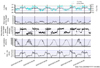 |
Figure 2 Markt Allhau: Sound level difference △LAeq, 250m and effective sound speed gradient with meteorological data wind speed, wind direction (0° correspond downwind sound propagation), net radiation and temperature gradient (10 m – 2 m) measured in K/m. |
For neutral meteorological conditions (−0.01 <  < +0.01), the measured values shown in Figure 2 result in a level reduction of ΔLA,eq, 250m = −22.4 dB(A).
2.4 Measurement location: railway line near Aderklaa
At the railway line near Aderklaa the sound emissions of the passing trains were measured in a flat region at a reference point at 25 m (a height of 3.5 m above the railway track, 4 m above ground) and at 100 m, 150 m, 250 m and 500 m on both sides of an almost straight track (at a height of at least 4 m above the nearest ground level, see Fig. 3). The GPS coordinates of the railway line are 48.294807, 16.527310 in decimal degrees. The entire region is almost entirely flat without any shielding objects or ground formations.
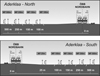 |
Figure 3 Railway line near Aderklaa with measurement positions north and south of the railway line. |
The choice of the measuring points to the north and south of the railway line meant that, in the event of variable meteorological conditions, upwind and downwind situations could be measured simultaneously on both sides.
Figures 4 and 5 includes the A-weighted sound exposure level differences ∆LA,E = LA,E,Xm − LA,E,25m for all the train passages at distances (X m = 100 m, 150 m, 250 m and 500 m) from the railway line relative to the reference point (25 m).
 |
Figure 4 Aderklaa: A-weighted sound exposure level differences ΔLA,E for the all train passages at different distances from the railway line relative to the reference point and meteorological data. |
 |
Figure 5 Aderklaa: Comparison of the sound exposure level difference (ΔLA,E) at different distances north and south of the railway line. |
Figure 4 shows the results for the measuring period from 31st August to 2nd September 2015 with the wind direction defined with respect to the perpendicular to the railway line (0° favourable downwind situation for southern points). Two hundred and fifty train passages were recorded during the 36-h period.
There was a high-pressure weather situation with conditions for the formation of an inversion layer (positive temperature gradient) at night and a strong unstable situation (negative temperature gradient) during the day. In the first night, there was a strong ground-level inversion that led to a strong reduction in the wind speed starting at 10 pm (decoupling of surface air flow from overlying air). The following day the wind speed increased creating highly unstable conditions. As a result of the increasing wind speed gradient during the day, favourable conditions for the southern acoustic measuring points appeared which are particularly well shown at the measuring point at a distance of 250 m (Fig. 5). There is a pronounced difference in the sound level differences developing between upwind and downwind measurements.
At the beginning of the second night, a positive temperature gradient was generated (inversion) which rapidly led to a significant decrease in the sound level differences, especially at the southern measurement point. Therefore, the sound level at all points and distances increased. The wind direction changed by about 45 degrees at this time which also contributed to the changes in sound levels. The second half of the night was characterised by the passage of a cold front just before midnight which led to the destruction of the ground-level inversion. Due to the frontal passage, the wind direction changed by 180° which led to changes in upwind and downwind sound propagation. Therefore, the wind direction and the wind speed gradient are the important quantities to interpret the sound level. This can be seen very clearly at the distance of 250 m. The measurements at the other distances show this effect too (see Fig. 5).
The sound attenuation in Figure 5 clearly shows the distance effect and the influence of the wind direction. During daytime conditions (unstable situation), the sound level difference is approximately 5 dB(A) at 100 m distance and increases to about 10 dB(A) at 250 m. The results for 500 m are limited as they were already strongly influenced by background noise especially for unfavourable sound propagation conditions resulting in only a few useable data points (>8 dB(A) than ambient noise).
2.5 Measurement location: Motorway A2 (Suedautobahn) near Bad Voeslau
At the motorway (A2) near Bad Voeslau (see Fig. 6), the sound levels of road traffic noise were measured during a 60-h period at reference points on both sides of the motorway at a distance of 200 m from the motorway and with a reference point at a distance of 34 m from the motorway. The GPS coordinates of the motorway are 47.975423, 16.249248 in decimal degrees. In contrast to the previous measurement sites, the road is slightly curved which is still considered to be negligible for the sound propagation up to the relevant 200 m. The measurements took place on both sides of the motorway at a height of 4 m above the motorway over the period from 19th to 22nd April 2016.
 |
Figure 6 Motorway measurement location near Bad Voeslau. |
Figure 7 shows the A-weighted equivalent sound level difference (ΔLA,eq,200m = LA,eq,200m − LA,eq,34m) on both sides of the motorway as a function of time.
 |
Figure 7 Bad Voeslau: ΔLA,eq,200m and the effective sound speed gradient on both sides of the motorway with meteorological data. |
The wind direction is shown in such a way that 0° represents a favourable sound propagation situation for the south. This measurement period was characterised by strong winds in the first night and day periods with a lack of temperature gradients and in the subsequent night-day period by low winds and strong temperature gradients. The first night from the 19th to the 20th of April was characterised by strong northern winds and overcast skies. This situation resulted in only slight temperature gradients but strong wind gradients. This resulted in considerable differences in sound levels between north and south whereby the southern measuring point was very favourable in terms of wind and resulted in differences in sound levels of 6 to 8 dB in the first night. On the first day of the test period there was a strong upwind situation for the southern measuring point and a difference in A-weighted sound level between the two measuring points (north and south) of about 10 dB resulted. The second night was characterised by clear sky conditions combined with a strong ground-level inversion. This caused low wind speed in the measurement profile whereby the wind came from the west and was parallel to the motorway. On the third night, a similar meteorological situation was observed with low sound level differences between the northern and southern measuring points.
In strong winds, there are large differences in the sound levels between upwind and downwind sound propagation. The time-dependent coincidence between the gradients of the effective sound speed and the sound level difference can be seen well in this measurement period (see Fig. 7). The highest sound level of the entire measuring period is noticeable in the case of downwind on the first day (20th April).
2.6 Comparison of the meteorological situation of Aderklaa and Bad Voeslau
The meteorological situations of Aderklaa (Fig. 4) and Bad Voeslau (Fig. 7) differed significantly. There was a much stronger wind (upwind and downwind) in Bad Voeslau than in Aderklaa which meant that acoustic measurements could be made in a wider range of  (see Tab. 1).
Comparison of the (average) meteorological data of Bad Voeslau and Aderklaa.
In Bad Voeslau there is a range of  (range −0.6 <
  < +0.5 1/s) and it has been shown that larger gradients (see Sect. 3.1) are mainly influenced by the wind.
3 Results and model approach of the S-shaped function
3.1 Sound attenuation and effective wind speed gradient
In the following diagrams, the sound attenuation is shown as a function of the effective sound speed gradient. The distribution of the data points indicates which effective sound speed gradients occurred most frequently during the individual measurement period.
The gradient of the effective sound speed  consists of two contributing factors; the temperature gradient and the wind speed gradient (see Eq. (2)). To analyse the different contributions of the temperature and wind gradients to the effective sound speed gradient, the normalized wind speed gradient
  is introduced and calculated with:
 (3)
(3)
and presented in Figure 8 for Aderklaa and Figure 9 for Bad Voeslau.
 |
Figure 8 Bad Voeslau: The uppermost diagram shows the normalized wind speed gradient ( |

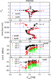 |
Figure 9 Aderklaa: The uppermost diagram shows the normalized wind speed gradient ( |


If  converges towards zero, the effective wind speed gradient
  converges to infinite (Eq. (3)). When
  is close to zero, it is mainly caused by the temperature gradient. The temperature gradient T′ and the effective sound speed gradient
  can have different signs and thus a very wide range of values (for example −4 <
  < 6 for Aderklaa) is possible for the effective wind speed gradient
  . If the temperature gradient T′ is small compared to
  , then
  converges to 1.
Figure 8 provides an overview of all the data points from the measurement sides of both sides of the motorway. A distinction is made between the southern and northern measuring points. The uppermost diagram of Figure 8 shows the share of the wind gradient  versus
  . The middle figure depicts the temporal distribution of
  . The bottom graph shows the sound level difference ΔLA,eq as a function of the effective sound speed gradient.
An essential difference between both measurements was a much stronger wind contribution at the road site in Bad Voeslau (see Tab. 1). At the road measurement location, the proportion of the wind gradient shows that the gradients outside the range −0.2 <  < 0.2 1/s are a result of the wind speed gradient (see the topmost diagram of Fig. 8). From the figure, it follows that the gradients −0.2 1/s <
  < 0.2 1/s are mainly influenced by the temperature gradient. From the time series plot of Figure 7 it is obvious that large gradients occurred during the night and day at the beginning of the measurement period. Smaller gradients (−0.2 1/s <
 < 0.2 1/s) were found during the day and the night near the end of the measurement period.
The northern measurement points have quite large negative gradients at the beginning of the measuring period which leads to a significant sound level attenuation due to the upward refracted sound rays (see Fig. 8). The southern measurement points have a downwind situation and thus only minor sound level changes.
Analogous to Figures 8 and 9 shows the proportion of the wind speed gradient  to the effective sound speed gradient (
 ) for Aderklaa to demonstrate the influence of the wind speed gradient. In the two lower diagrams of Figure 9, the sound attenuation is shown as a function of the effective sound speed gradient
  for the distances 100 m, 250 m and 500 m.
At the Aderklaa measurement location (Fig. 9), the wind speed was rather low (see Tab. 1). The middle diagram of Figure 9 shows at which points in time the different gradients were present. It is shown that  > 0 was found in the first and second nights, while
  < 0 was found during the daytime of the first and second days. Upwind and downwind sound propagation situations have been documented (measurements on both sites of the railway line). Large gradients, because of a high wind speed, are found on the second day at the end of the measurement period (see Fig. 9).
Figure 9 shows that the temperature gradient played an essential role in Aderklaa while the wind gradient played a rather subordinate one. The temperature gradient had the same influence on the southern and northern measuring points whereas the wind, with its changes of speed and direction (see Fig. 4), influenced the southern and northern measuring points differently. Figure 4 also shows that wind speeds below 2 m/s at a height of 10 m have only minor influence on the sound level. Figure 5 shows very clearly how the wind at a distance of 100 m has only a very small influence and with increasing distance from the sound source it influences the sound attenuation more and more. In Aderklaa single train passages were measured and there it can be seen that the wind speed and direction influences the scattering of the acoustic measuring points and that the scattering increases with increasing distance (see Figs. 5 and 9). Figure 9 also shows that the diurnal course of the gradient is crossed by a change in wind direction during the second night.
3.2 Model approach from the measurements: S-shaped sound attenuation
The analysis of the measurement results in Section 3.1 shows that  close to 0 is mainly influenced by the temperature gradient while larger gradients are mainly influenced by the wind gradient. An S-shaped function (or sigmoid function) describes that the sound level differences are constant for large positive gradients (
 ) with sound ray refraction downwards and large negative gradients (
 ) with sound ray refraction upwards.
The S-shaped function according to reference [10] is slightly modified to:
 (4)
(4)
where the value LL (lower limit) is the average lower sound level at large negative gradient, H is the difference between average lower (LL) and higher sound levels (UL, upper limit), b represents the left/right offset and a includes the slope of the S-shaped function. Equation (4) implies that the sound level difference ∆L(d,  ) takes a constant value for very large and very small gradients. In case of
  = 0 ΔL(d, 0) is dependent on distance, atmospheric attenuation, ground effects and diffraction, only. Figure 10 show the sound level difference ΔLA,eq as a function of effective sound speed gradients. Figure 11 shows ∆LA,E versus
  of for three different distances. While in the datasets of Markt Allhau (Fig. 10) and in Bad Voeslau (Fig. 12) the definition of LL is clear, in Aderklaa (Fig. 11) the variation of the sound level difference is large for
  < 0 due to a low number of data points with strong upwind. The mentioned figures also show that ∆L(d, 0) can be calculated from the available measured values for the range around gradient
  ~ 0, (Bad Voeslau and Aderklaa: −0.05 ≤
  ≤ 0.05 1/s, Pinkafeld: −0.025 ≤
  ≤ 0.025 1/s). For
  > 0 the averaged sound level differences are named upper limit (UL). The upper limit, which is the horizontal asymptote, was iteratively defined as the arithmetic mean of all upper datapoints which resulted in a constant value.
 |
Figure 10 Markt Allhau: Sound level difference ΔLA,eq versus effective sound speed gradient ( |

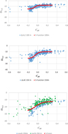 |
Figure 11 Aderklaa: Sound exposure level difference ΔLA,E versus effective sound speed gradient for different distances from the railway line with calculated S-shaped function. |
 |
Figure 12 Bad Voeslau: Sound level difference ΔLA,eq dependent on effective sound speed gradient ( |

Introducing ∆L(d, 0), equation (5) can be transformed to:
 (5)
(5)
Using the least square fit between data and equation (5) (CurveFit of MATLAB, The Mathworks, USA), parameters a, b and LL were determined (Tab. 2).
Summary of different constants (derived from measurement results) for the calculation of the S-shaped function. Sound attenuation without meteorological influences ∆L(d, 0), because of meteorological influences H and for favourable ( > 0) and unfavourable (
 < 0) sound propagation.
The sound level difference ∆L(d, 0) represents the sound level at distance d from the sound source at neutral meteorological conditions ( = 0). The difference |∆L(d, 0) − UL| is the level increase under favourable sound propagation conditions. The difference |∆L(d, 0) − LL| is the level reduction related to
  = 0 under unfavourable sound propagation conditions. The value H is the observed spread due to the meteorological influence at the different measurement points. The values of UL and LL in relation to ∆L(d, 0) show that the S-shaped function is not symmetric with respect to ∆L(d, 0) (see Tab. 2 and Figs. 10–12). The coefficient of determination R2 in Table 2 for Markt Allhau shows the lowest correlation (R2 = 0.33) because of the two-month measurement duration in combination with small meteorological effects (wind direction parallel to the motorway) as well as changing ground conditions during the vegetation period.
The calculated S-shaped functions with the parameters of Table 2 are shown in Figures 10–12 where the sound level differences dependent on  are presented for different measurement positions.
At the railway measurement location Aderklaa, the sound exposure level differences were measured on both sides of the railway line and thus upwind and downwind situations were recorded at different distances from the railway line.
Figure 11 shows a large range of variation in the measurement results at a distance of 250 m, especially for  < 0 with unfavourable sound propagation. In Figure 11, a systematic difference between the southern and northern measurement points can be seen at 250 m distance. The reason for this could be that north of the railroad line there was a windbreak belt with bushes and trees with a maximum height of 3 m. The measurement distance of 500 m is not included in this analysis because of the low number of valid data points.
For the motorway measurement site Bad Voeslau, Figure 12 shows that there was mainly downwind sound propagation north of the highway, whereas mainly upwind sound propagation in the south. At this measurement location, high wind speed caused a wide distribution of  and thus the wind effects on the sound propagation is evident. The distribution of the measured values also shows that the sound attenuation remains approximately constant for high wind speed.
4 Discussion of the S-shaped sound level attenuation
The effective sound speed gradients ( ) shown in Section 3.2 were determined from the temperature and wind speed gradients. The sound level attenuation dependent on effective sound speed gradient is approximated with an S-shaped function.
In the high wind case, the turbulence has a very dramatic impact both upwind and downwind. In the upwind direction, the turbulence scatters substantial sound energy in the shadow zone [5].
Chevret et al. [14] show in numerical calculations that the level distribution is strongly influenced by the turbulent atmosphere both in the free field and in upward refractive conditions. Due to the turbulence, the sound level can remain constant after about 100–200 m in upward-refracting conditions as is shown in [3] and [10] for f = 424 and 848 Hz.
The S-shaped function in Figures 13 and 14 are shown for all measurement locations dependent on the meteorological conditions expressed as  . The railway measurements at different distances at Aderklaa show a continuous behaviour in the distance ranges of 100 m, 150 m, and 250 m as presented in Figure 13 which also shows different courses of the S-shaped function depending on the distance from the sound source. Thus, the increasing influence of the meteorological conditions with increasing distance is shown. The results for this measurement site show an influence of the meteorological conditions (see Fig. 13 and Tab. 2) of 7 dB(A) at a distance of 100 m and about 13 dB(A) at a distance of 250 m. However, the S-shaped function did not reach its lower plateau, as can be seen in Figure 13.
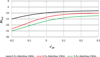 |
Figure 13 S-shaped sound attenuation versus |

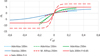 |
Figure 14 Sound level difference ∆L caused by the meteorological influences versus the effective sound speed gradient for the different measurement situations in the range of 100–250 m distance in comparison with the calculations of Salomons and Bakri [10] mentioned as Salo. |
Figure 14 shows a comparison of the measurement results in the range of 150–250 m from the sound source with the results of Salomons and Bakri [10]. They use the effective wind speed weff = ceff(10 m) − ceff(0 m) with ceff = c + u instead of  (see Eq. (2)) for the descriptions of meteorological situations. To be able to compare the S-function of Salomons and Bakri (Eq. (12) of [10]) the parameter A (see Tab. 3) and B = 10 dB is used.
Distance and height of the measurement points for calculation of factor F and the shift of the axis A.
The factor F of [10] is dependent on the geometrical parameters distance (horizontal source receiver distance) and the receiver height. Purely formally, the factors F and A of [10] correspond to the terms LL = F × A and H = F × B of equation (5) of this paper. The term A corresponds to the sound level difference at distance d without meteorological influences, referred in Table 2 as ∆L(d, 0).
At the location of Markt Allhau (Fig. 1) a small sound shielding were effective which is the reason that the S-shaped function of Markt Allhau has a lower sound level than the measurement sites of Bad Voeslau and Aderklaa (see ∆L(d, 0) in Tab. 2).
The results in Figure 14 show remarkable differences at the slope of the different S-functions. A steep increase of the S-shaped function means that there is only a small gradient range at this measuring point. Then, according to Section 3.1, it is the temperature gradient which is mainly effective. If the slope of the S-shaped function is flat, then a larger wind gradient is present at this measuring point. The higher wind speed at Bad Voeslau caused a flattening of the S-shaped function (Voeslau 200 m) as shown in Figure 14. In contrast to that the Aderklaa distribution with low wind speeds resulted in a steeper course S-shaped function (Fig. 14).
The constant values for large and small gradients correspond to a threshold which is determined by the meteorological conditions (mainly wind speed) at the respective measuring point as well as the geometry of the acoustic measurement set up.
For a better comparison of the different S-functions, the values in Figure 14 are related to ∆L(d, 0) (see Tab. 2), i.e. to the sound level attenuation without meteorological influences. This clearly shows a different level increase due to favourable sound propagation and the different level decrease due to unfavourable sound propagation.
The S-functions based on our measurement results show a broader gradient than the calculation results of Salomons and Bakri [10] which means that their gradients were assumed to be very close to  = 0.
= 0.
The main results of Figure 14 are summarized in Table 2. The maximum acoustic effects because of meteorological influence for  ≫ 0 and
  ≪ 0 are described in Salomons and Bakri [10] and agree approximately with our measurement results.
It was determined for the distance range of 150–250 m that the sound level increases by 3–4 dB(A) for favourable sound propagation and decreases by 5–10 dB(A) for unfavourable sound propagation when compared to situations without meteorological influence (see Tab. 2 and Fig. 14). The total meteorological influence on sound propagation in the distance range from 150 to 250 m is between 8.5 and 14 dB(A) (see Tab. 2). This agrees quite well with the results of Heimann and Salomons [4] who found a calculated level change of 9 dB at 200 m because of changing (measured) meteorological conditions.
The considerations presented here refer to a situation in which the emission line lies approximately in one plane with the receiver points. Therefore, our results are limited to situations without substantial noise attenuation due to screens.
5 Conclusion
The presented analysis for the A-weighted sound levels attenuation of road and railway traffic shows a strong correlation of the effective sound speed gradient  depending on the distance between 100 and 500 m.
The effective sound speed gradient  includes the temperature and vector wind gradient and changes due to the meteorological conditions during the course of a day. The measured datasets suggest that smaller gradients (−0.2 <
  < 0.2 1/s) are mainly due to temperature gradient while larger gradients are usually due to wind gradients with upwind or downwind sound propagation.
The A-weighted sound attenuation dependent on  fits to a S-shaped function. This means that the sound level difference is constant for a certain value of
  for unfavourable and favourable sound propagation. When compared to a situation without meteorological influence (
 ~ 0), the sound level increases by 3–4 dB(A) for downward refracted sound rays (favourable sound propagation) and decreases by 5–10 dB(A) for upward refracted sound rays (unfavourable) in the distance range of 150–250 m.
The slope of the S-shaped function is a result of the different meteorological conditions especially the higher upwind and downwind speeds which led to higher average gradients for  . High wind speeds result in high wind gradients and low temperature gradients (turbulent mixing). The different meteorological conditions can be the result of geography and local topography which are only accessible by microscale meteorological data (or measurement on site).
With the proposed S-shaped function it is possible to find upper and lower limits of the sound level at certain distances from the noise source. The upper and lower thresholds are mainly affected by geometrical parameters (acoustic source-receiver configuration including ground and shielding) and the wind speed gradient which is responsible for large values of the effective sound speed gradients  .
.
Acknowledgments
The present work is based on the research project ACUMET [15] funded by the Austrian Federal Railways Infrastructure AG (ÖBB), Austrian Motorway Operator (ASFINAG) and Federal Ministry of Transport, Innovation and Technology (BMVIT) and organized by the Austrian Research Promotion Agency (FFG). Within this research project, Bernhard Streit helped us with the evaluation and the presentation of the results. Thomas Loewenpast helped us with the calculation of the S-shaped function.
Many thanks also to the two anonymous reviewers who worked intensively on the paper and contributed many valuable comments on a previous version. We would like to thank both reviewers who contributed significantly to improving the quality of this paper.
Conflict of interest
The authors declare that they have no conflicts of interest in relation to this article.
References
- D. Heimann, E. Salomons: Testing meteorological classifications for the prediction of long-term average sound levels. Applied Acoustics 65 (2004) 925–950. https://doi.org/10.1016/j.apacoust.2004.05.001. [CrossRef] [Google Scholar]
- R.B. Stull: An introduction to boundary layer meteorology, atmospheric science library. Kluwer Academic Publishers, Reprint Dordrecht, The Netherlands, Chap. 5, 1994, pp. 151–196. [Google Scholar]
- K. Attenborough, T. van Renterghem: Predicting outdoor sound, Second edition. CRC Press, Taylor & Francis, Chap. 1, 2021. [CrossRef] [Google Scholar]
- E.M. Salomons: Computational atmospheric acoustics. Kluwer Academic Publisher, Dordrecht, The Netherlands, Chap. 4, 2001, pp. 37–66. [CrossRef] [Google Scholar]
- V.E. Ostashev, D.K. Wilson: Acoustics in moving inhomogeneous media, Second edition. CRC Press, Taylor & Francis Group, Boca Raton, London, New York, Chap. 3, 2016, pp. 63–106, Chap. 11.2, pp. 404–425. [Google Scholar]
- D. Hohenwarter, E. Mursch-Radlgruber: Nocturnal boundary layer profiles and measured frequency dependent influence on sound propagation. Applied Acoustics 76 (2014) 416–430. [CrossRef] [Google Scholar]
- D. Hohenwarter, F. Jelinek: Snell’s law of refraction and sound rays for a moving medium. Acta Acustica 86 (2000) 1–14. [Google Scholar]
- V.E. Ostashev, D. Hohenwarter, K. Attenborough, Ph Blanc-Benon, D. Juvé, G.H. Goedecke: On the refraction law for a sound ray in a moving medium. Acta Acustica 87 (2001) 303–306. [Google Scholar]
- B. Rayleigh, J.W. Strutt: The theory of sound. Dover Publications, New York, Chap. 289 (Refraction by wind), 1945, pp. 132–134. Unabridged republication of the second revised and enlarged edition of 1896.s [Google Scholar]
- E.M. Salomons, T. Bakri: Fluctuating traffic noise levels calculated from time-dependent traffic data: An engineering approach. Noise Control Engineering Journal 66, 5 (2018) 432–445. [CrossRef] [Google Scholar]
- ISO 1996-1: Acoustics – description, measurement and assessment of environmental noise – part 1: Basic quantities and assessment procedures. 2016. [Google Scholar]
- V. Zouboff, Y. Brunet, E. Sechet, J. Bertrand: Validation d’une méthode qualitative d’estimation de l’influence de la météorologie surle bruit. Journal de Physique IV Colloque C5, Supplément au Journal de Physique III 4 (1994) C5-813–C5-816. [Google Scholar]
- D.K. Wilson: The sound-speed gradient and refraction in the near-ground atmosphere. Journal of the Acoustical Society of America 113 (2003) 750–757. [CrossRef] [PubMed] [Google Scholar]
- P. Chevret, Ph Blanc-Benon, D. Juvè: A numerical model for sound propagation through a turbulent atmosphere near the ground. Journal of the Acoustical Society of America 100, 6 (1996) 3587–3599. [CrossRef] [Google Scholar]
- C. Kirisits, E. Mursch-Radlgruber, D. Hohenwarter, B. Streit: Analyse und Berücksichtigung des Einflusses der Meteorologie auf die Schallausbreitung von Bahn-und Straßenverkehrslärm. ACUMET, Herausgeber Bundesministerium fuer Verkehr, Innovation und Technologie, 1030 Wien, 2016. (in German). https://www2.ffg.at/verkehr/studien.php?id=1224&lang=de&browse=sxckiumr. [Google Scholar]
Cite this article as: Hohenwarter D. Mursch-Radlgruber E. & Kirisits C. 2022. S-shaped dependence of the sound pressure level in outdoor propagation on the effective sound speed gradient. Acta Acustica, 6, 13.
All Tables
Summary of different constants (derived from measurement results) for the calculation of the S-shaped function. Sound attenuation without meteorological influences ∆L(d, 0), because of meteorological influences H and for favourable ( > 0) and unfavourable ( < 0) sound propagation.
Distance and height of the measurement points for calculation of factor F and the shift of the axis A.
All Figures
|
Figure 1 Markt Allhau: MP 250 m is 3 m under the surface of the motorway. |
| In the text | |
|
Figure 2 Markt Allhau: Sound level difference △LAeq, 250m and effective sound speed gradient with meteorological data wind speed, wind direction (0° correspond downwind sound propagation), net radiation and temperature gradient (10 m – 2 m) measured in K/m. |
| In the text | |
|
Figure 3 Railway line near Aderklaa with measurement positions north and south of the railway line. |
| In the text | |
|
Figure 4 Aderklaa: A-weighted sound exposure level differences ΔLA,E for the all train passages at different distances from the railway line relative to the reference point and meteorological data. |
| In the text | |
|
Figure 5 Aderklaa: Comparison of the sound exposure level difference (ΔLA,E) at different distances north and south of the railway line. |
| In the text | |
|
Figure 6 Motorway measurement location near Bad Voeslau. |
| In the text | |
|
Figure 7 Bad Voeslau: ΔLA,eq,200m and the effective sound speed gradient on both sides of the motorway with meteorological data. |
| In the text | |
|
Figure 8 Bad Voeslau: The uppermost diagram shows the normalized wind speed gradient ( |
| In the text | |
|
Figure 9 Aderklaa: The uppermost diagram shows the normalized wind speed gradient ( |
| In the text | |
|
Figure 10 Markt Allhau: Sound level difference ΔLA,eq versus effective sound speed gradient ( |
| In the text | |
|
Figure 11 Aderklaa: Sound exposure level difference ΔLA,E versus effective sound speed gradient for different distances from the railway line with calculated S-shaped function. |
| In the text | |
|
Figure 12 Bad Voeslau: Sound level difference ΔLA,eq dependent on effective sound speed gradient ( |
| In the text | |
|
Figure 13 S-shaped sound attenuation versus |
| In the text | |
|
Figure 14 Sound level difference ∆L caused by the meteorological influences versus the effective sound speed gradient for the different measurement situations in the range of 100–250 m distance in comparison with the calculations of Salomons and Bakri [10] mentioned as Salo. |
| In the text | |
Current usage metrics show cumulative count of Article Views (full-text article views including HTML views, PDF and ePub downloads, according to the available data) and Abstracts Views on Vision4Press platform.
Data correspond to usage on the plateform after 2015. The current usage metrics is available 48-96 hours after online publication and is updated daily on week days.
Initial download of the metrics may take a while.