| Issue |
Acta Acust.
Volume 9, 2025
|
|
|---|---|---|
| Article Number | 52 | |
| Number of page(s) | 15 | |
| Section | Structural Acoustics and Vibroacoustics | |
| DOI | https://doi.org/10.1051/aacus/2025036 | |
| Published online | 12 August 2025 | |
Scientific Article
Impacts of pressure and pre-stress loads on the vibroacoustic response of laminated composite structures
1
School of Mechanical Engineering, Universiti Sains Malaysia, Nibong Tebal, 14300, Malaysia
2
Department of Mechanical Engineering, Federal University of Technology, PMB 704 Akure, Nigeria
3
Department of Mechanical Engineering, Faculty of Technology, KU Leuven, 9000
Gent, Belgium
* Corresponding author: This email address is being protected from spambots. You need JavaScript enabled to view it.
Received:
17
March
2025
Accepted:
12
July
2025
Abstract
This study investigates the effects of tensile pre-stress, compressive pre-stress, and surface pressure loads on the vibroacoustic behavior of laminated composite panels using a wave-based Statistical Energy Analysis (SEA) framework. A Wave Finite Element (WFE) method is used to compute wave dispersion, which informs the calculation of modal density, acoustic radiation efficiency, and sound transmission loss (STL). The numerical framework is validated against benchmark experimental and numerical results, with maximum discrepancies below 10%. Results reveal that tensile pre-stress decreases dispersion and modal density while shifting the coincidence frequency downward – from 15.2 kHz (0 N) to 5.1 kHz (100 N). In contrast, compressive pre-stress increases modal density and raises the coincidence frequency, reaching 108.5 kHz at 400 N. Surface pressure primarily affects low-frequency dynamics, increasing dispersion and reducing modal density, with STL coincidence frequency shifting from 12 kHz (0.6 GPa) to 20 kHz (0 GPa). Under combined loading, the dynamic response is intermediate, with pre-stress modulating the out-of-plane stiffening effect of pressure. These results offer critical insight for tailoring vibroacoustic performance in lightweight composite structures, particularly in aerospace and transport systems subjected to operational loading.
Key words: Wave finite element / Structural energy analysis / Pre-stressing / Pressurization / Vibroacoustic properties
© The Author(s), Published by EDP Sciences, 2025
 This is an Open Access article distributed under the terms of the Creative Commons Attribution License (https://creativecommons.org/licenses/by/4.0), which permits unrestricted use, distribution, and reproduction in any medium, provided the original work is properly cited.
1. Introduction
Laminated composite structures, including chamber-core and grid-stiffened configurations, have become integral to high-performance applications in the aerospace and automotive industries due to their exceptional stiffness-to-weight ratio, superior damping characteristics, and structural adaptability [1]. Notably, modern airframes such as the Airbus A350 XWB and Boeing 787 Dreamliner incorporate advanced composite materials, constituting approximately 80% of their total volume [1]. In the transportation sector, these materials play a notable role in the fabrication of high-speed trains, offering advantages such as lightweight construction, excellent tensile strength, enhanced stability, corrosion resistance, and superior acoustic insulation properties [2]. Despite these advantages, composite structures often exhibit suboptimal acoustic performance, leading to increased sound transmission, particularly under varying operational conditions [3, 4]. Addressing this limitation requires a comprehensive understanding of the influence of factors such as pre-stressing and pressurization on the vibroacoustic behavior of composite structures to optimize their design for improved structural and acoustic performance.
Accurate vibroacoustic modeling is a fundamental challenge in the optimal design of composite structures [5]. The predictive accuracy of numerical models is often hindered by uncertainties in material properties, boundary conditions, and operational loading parameters.Various studies have examined the influence of mechanical loading conditions on laminated composites. For instance, pre-stress conditions can alter structural stiffness and wave dispersion properties, influencing impact resistance and energy dissipation [6]. Preloading curved laminates increases curvature, leading to greater impact force and larger damaged regions [7]. Moreover, fluid-structure interaction in composite cylinders has been shown to affect vibroacoustic behavior based on parameters such as fluid height, fiber orientation, and shell dimensions [8]. Experimental results have also highlighted the impact of gradient residual stress and prestressed CFRP reinforcements on composite interfaces and joints [9, 10]. Additionally, the integration of nonlinear spring-mass systems and tensegrity-inspired layouts has shown promise in passive and active vibration reduction of complex assemblies [11, 12]. Collectively, these studies highlight the complex interplay between structural and environmental factors in determining the vibroacoustic response of laminated composites. However, the combined effects of pre-stress and pressure loads on wave propagation and acoustic performance remain insufficiently explored.
Significant progress has been made in modeling the vibroacoustic behavior of laminated composites, particularly in wave propagation analysis. The dispersion properties of composite structures are central to optimizing their vibroacoustic response [13, 14]. Energy-based methods such as the SEA approach have been employed to model vibroacoustic behavior in curved panels [15] and cylindrical composite structures [16]. Hybrid approaches integrating Boundary Element Method (BEM) with FiniteElement (FE) analysis have also been explored [17], alongside artificial intelligence-based optimization methods using neural networks [18, 19]. Recent advances also include time-domain damping formulations for vibration response prediction [20], as well as noise cancellation strategies using active control techniques [21] and Doppler assimilation [22]. Despite their accuracy, full-scale FE models remain computationally prohibitive for large composite structures [23]. To address these limitations, the Wave Finite Element (WFE) method has been introduced as a computationally efficient alternative, providing rapid dispersion analysis while maintaining high accuracy [23, 24].
The WFE method is an efficient approach for analyzing vibroacoustic characteristics of composite structures. It combines wave propagation theory with finite element modeling to study complex laminated structures [25]. The method has been applied to various scenarios, including composite honeycomb panels [26, 27] and cross-laminated panels [28]. The WFE method can accurately predict dispersion relations, mode shapes, and sound transmission loss in multi-layered panels, offering advantages over simplified plate models [29]. It also supports modeling ofviscoelasticity, nonlocal effects, and fluid-structure interactions [30, 31]. The method is computationally efficient and provides accurate results for a wide range of frequencies [25, 32]. WFE has shown good agreement with experimental measurements, making it a valuable tool for optimizing the design of composite structures for vibroacoustic performance [32].
In contrast to previous studies that primarily address vibroacoustic behavior in laminated sandwich panels or cylindrical shells under single types of operational loads, this study presents a unified framework that simultaneously considers the effects of both in-plane pre-stress and surface pressure loads on finite laminated composite panels. For instance, Manconi et al. [33] investigated residual stress and internal fluid loading in laminatedcylinders using a similar WFE-SEA methodology, but did not explore combined external pressurization and in-plane loading in flat panels. Similarly, Yang et al. [34] and Cool et al. [35] evaluated STL in periodic or layered structures, focusing on structural configurations and loading conditions different from those addressed here.
The key novelty of this work lies in integrating dispersion analysis of the fundamental antisymmetric Lamb wave mode (A0 mode) – computed via the Wave Finite Element method – within a Statistical Energy Analysis framework to assess the combined influence of pressure and pre-stress on vibroacoustic performance. This includes detailed computation of modal density, radiation efficiency, and transmission loss as functions of load parameters. A finite laminated composite panel is analyzed, and the results are used to explore how varying levels of tensile/compressive pre-stress and pressurization affect the coincidence frequency and broadband acoustic response. The combined treatment of these two loading conditions is particularly relevant for aerospace and transport applications, where both surface pressure (e.g., due to cabin pressurization) and pre-stress (e.g., from manufacturing or thermal mismatch) co-exist and influence design performance. The findings also offer valuable contributions to the design and predictive modeling of lightweight composite structures, particularly in aerospace and high-speed transportation applications where vibroacoustic performance is a critical design consideration.
2. Stiffness properties of laminated composite structure under pressure and pre-stress loads
A laminated composite waveguide (Fig. 1) subjected to uniform pressure and in-plane pre-stress loads is considered in this study. In the finite element (FE) formulation, additional stiffness matrices representing the stiffening effects due to these loads are incorporated into the total stiffness matrix. The total stiffness matrix K is expressed as:
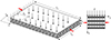 |
Figure 1. Configuration of a laminated composite under pressure and pre-stress (compression) loads. |
 (1)
(1)
where K 0 is the structural stiffness matrix of the unstressed and unpressurized composite panel, K P is the pressure-induced geometric stiffness matrix, and K S is the pre-stress-induced geometric stiffness matrix.
Assuming small deformations and geometrically linear behavior (i.e., within the pre-buckling regime), both K S and K P can be approximated as linear functions of the applied loads:
 (2)
(2)
where
σ
0
is the uniform in-plane pre-stress (tensile or compressive), p is the uniform surface pressure, and  and
and  are geometric stiffness matrices precomputed for unit pre-stress and unit pressure, respectively.
The geometric stiffness matrix K S resulting from pre-stress is formulated based on the stress-stiffening effect as [27]:
 (3)
(3)
where S is the shape function derivative matrix and τ is the Cauchy stress tensor. When τ corresponds to a uniform axial or biaxial pre-stress σ 0 , and the structural configuration remains fixed, the resulting integral yields a geometric stiffness matrix that varies linearly with σ0.
This parametric formulation enhances the computational efficiency of the wave-based approach, enabling rapid re-evaluation of wave dispersion and vibroacoustic quantities over a wide range of pre-stress and pressure loading conditions.
3. Wave-based SEA computation of vibroacoustic quantities
A wave-based scheme in the SEA context for computing the vibroacoustic quantities of laminated waveguides is presented in this section. The scheme calculates the wave propagation characteristics of the waveguide using the WFE approach. The numerically computed dispersion characteristics of the fundamental antisymmetric Lamb wave mode (A 0 mode) are then applied, in the SEA context, to calculate the vibroacoustic quantities of the laminated structure.
3.1. WFE computation of wave dispersion properties
Two-dimensional wave motion is considered in the x and y directions of a laminated composite waveguide under pressure and pre-stress loads, as shown in 1. The dimension of the waveguide is Lx × Ly × t. Taking advantage of the periodicity of the waveguide, a small periodic segment ABCD (Fig. 1) of dimension δx × δy × t is modelled using a commercial FE software, ANSYS . The stiffness matrices (K
0
, K
P
, K
S
) and hence the total stiffness matrix K and the mass matrix M of the modelled segment are computed using classical FE algorithms.
. The stiffness matrices (K
0
, K
P
, K
S
) and hence the total stiffness matrix K and the mass matrix M of the modelled segment are computed using classical FE algorithms.
Assuming a time-harmonic behavior for the wave motion, the equation of motion can be expressed as [23]:
 (4)
(4)
where D is the dynamic stiffness matrix (DSM), q is the displacement vector containing all degrees of freedom (DoF) and F is the nodal force vector and. The DSM is expressed as [24]:
 (5)
(5)
where ξ is the structural damping, which is uniform for all DoF of the structural segment and ω is the angular frequency. Equation (5) can be partitioned into the predefined sequence ABCD of the modelled segment as:
![Mathematical equation: $$ \begin{aligned} \left[ \begin{array}{llll} \mathbf{D }_{\mathrm{AA} }&~~ \mathbf{D }_{\mathrm{AB} }&~~ \mathbf{D }_{\mathrm{AC} }&~~ \mathbf{D }_{\mathrm{AD} }\\ \mathbf{D }_{\mathrm{BA} }&~~ \mathbf{D }_{\mathrm{BB} }&~~ \mathbf{D }_{\mathrm{BC} }&~~ \mathbf{D }_{\mathrm{BD} }\\ \mathbf{D }_{\mathrm{CA} }&~~ \mathbf{D }_{\mathrm{CB} }&~~ \mathbf{D }_{\mathrm{CC} }&~~ \mathbf{D }_{\mathrm{CD} }\\ \mathbf{D }_{\mathrm{DA} }&~~ \mathbf{D }_{\mathrm{DB} }&~~ \mathbf{D }_{\mathrm{DC} }&~~ \mathbf{D }_{\mathrm{DD} }\\ \end{array} \right]\left\{ {\begin{array}{l} \mathbf{q }_{\mathrm{A} } \\ \mathbf{q }_{\mathrm{B} } \\ \mathbf{q }_{\mathrm{C} } \\ \mathbf{q }_{\mathrm{D} } \\ \end{array}} \right\} = \left\{ {\begin{array}{l} \mathbf{F }_{\mathrm{A} } \\ \mathbf{F }_{\mathrm{B} } \\ \mathbf{F }_{\mathrm{C} } \\ \mathbf{F }_{\mathrm{D} } \\ \end{array}} \right\} . \end{aligned} $$](/articles/aacus/full_html/2025/01/aacus250027/aacus250027-eq9.gif) (6)
(6)
Using the Bloch’s theorem for the modelled segment, under the assumption of a time harmonic response, the displacements and forces at the edges of the segment can be expressed with reference to one of the edges. Using the edge D as a reference, the displacement and force vectors can be expressed as [24]:
![Mathematical equation: $$ \begin{aligned} \left\{ {\begin{array}{l} \mathbf{q }_{\mathrm{A} } \\ [2pt] \mathbf{q }_{\mathrm{B} } \\ [2pt] \mathbf{q }_{\mathrm{C} } \\ [2pt] \mathbf{q }_{\mathrm{D} } \\ \end{array}} \right\} =\left\{ {\begin{array}{c} {\varepsilon }_{{x}}{\varepsilon }_{{y}}\mathbf{I } \\ [2pt] {\varepsilon }_{{y}}\mathbf{I } \\ [2pt] {\varepsilon }_{{x}}\mathbf{I } \\ [2pt] \mathbf{I } \\ \end{array}} \right\} \mathbf{q }_{\mathrm{D} },~~ \left\{ {\begin{array}{l} \mathbf{F }_{\mathrm{A} } \\ [2pt] \mathbf{F }_{\mathrm{B} } \\ [2pt] \mathbf{F }_{\mathrm{C} } \\ [2pt] \mathbf{F }_{\mathrm{D} } \\ \end{array}} \right\} =\left\{ {\begin{array}{c} {\varepsilon }_{{x}}{\varepsilon }_{{y}}\mathbf{I } \\ [2pt] {\varepsilon }_{{y}}\mathbf{I } \\ [2pt] {\varepsilon }_{{x}}\mathbf{I } \\ [2pt] \mathbf{I } \\ \end{array}} \right\} \mathbf{F }_{\mathrm{D} } \end{aligned} $$](/articles/aacus/full_html/2025/01/aacus250027/aacus250027-eq10.gif) (7)
(7)
where ε x and ε y are the wave propagation constants, related to the propagation wavenumbers k x and k y as [23]:
 (8)
(8)
Assuming a free wave propagation, equilibrium at any edge implies that the sum of forces of all edges connected to the edge equal to zero. Taking equilibrium at the reference edge D, then
 (9)
(9)
Substituting the displacement vector in equation (8) and the equilibrium expression in equation (10) into equation (7) and solve the resulting equation completely, then a quadratic eigenproblem is obtained as
 (10)
(10)
where
 (11)
(11)
The solution of the quadratic eigenproblem (Eq. (11)) yields the propagation constants along the x direction. Corresponding expressions can be obtained for the propagation constants in the y direction, by making ε y the subject. The wavenumbers are computed as [23]:
 (12)
(12)
The wave dispersion analysis focuses on the fundamental antisymmetric Lamb wave mode (A 0 mode), which dominates out-of-plane flexural motion in thin composite panels. The computed wavenumbers include the propagating component. An algorithm is implemented to isolate the propagating wavenumbers corresponding to the A 0 mode by using the modal assurance criterion (MAC) across frequencies. This filtering is essential for computing vibroacoustic properties relevant to radiation and STL performance.
Higher-order symmetric or shear-dominated wave modes are excluded from the SEA formulation, as they contribute minimally to far-field acoustic radiation in the targeted frequency range for typical panel thicknesses(1–10 mm). The focus on the A 0 mode is justified based on its dominant role in low-to-mid frequency vibroacoustic transmission in laminated structures.
The computed wavenumbers k x (ω, p, σ 0 ) and k y (ω, p, σ 0 ) are functions of angular frequency, applied pressure p, and pre-stress load σ 0 .
In this study, structural damping is introduced via a uniform loss factor ξ, which is incorporated into the dynamic stiffness matrix to account for energy dissipation. As a result, the computed wavenumbers are generally complex. The inclusion of damping plays a key role in the classification of wave modes, particularly in distinguishing propagating modes from evanescent and attenuating ones. This sorting is essential for ensuring that only physically meaningful, radiating wave modes are retained for subsequent vibroacoustic calculations.
To compute modal density and group velocity, the absolute value (|k|) of the complex wavenumber is used and the group velocity is then calculated as dω/d|k|, as shown in equation (14). Equation (14) remains valid under these conditions by computing the group velocity with respect to the magnitude of the complex wavenumber, which is a standard practice in wave-based SEA modeling under light damping conditions (e.g., [36]). This approach ensures that all resulting quantities – such as modal density, radiation efficiency, and sound transmission loss – remain real and physically interpretable. While damping has a minimal effect on wave dispersion due to its small magnitude, it plays a significant role in shaping peak responses, especially around resonance and coincidence frequencies.
3.2. SEA computation of vibroacoustic quantities
The vibroacoustic performance of the laminated waveguide is considered by computing the acoustic transmission coefficients of the waveguide in-between two acoustic cavities (Fig. 2). One of the cavities is acoustically excited and acoustic energy transmission through the waveguide to the other cavity is computed using the SEA approach. The considered vibroacoustic performance quantities include the modal density, radiation efficiency and sound transmission loss.
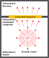 |
Figure 2. Schematic representation of acoustic transmission in the statistical energy analysis context. |
3.2.1. Modal density calculation
The angle-dependent modal density for the pressurized and pre-stressed layered waveguide is computed in terms of the ratio of the wavenumber of the fundamental antisymmetric Lamb wave mode (A 0 mode) to the corresponding group velocity as [37]:
 (13)
(13)
where A is the area of the layered waveguide and φ is the heading angle, which ranges from 0 to π. The group velocity c g is given by Chronopoulos et al. [3]:
 (14)
(14)
Equation (16) is then angularly averaged by integrating it over the heading angles to calculate the modal density as a function of ω, p and s:
 (15)
(15)
3.2.2. Radiation efficiency calculation
Using the Leppington’s asymptotic formulas [38, 39] and assuming energy equipartition for the resonant modes in the context of SEA, the acoustic radiation efficiency σ(ω,p,s) for the pressurized and pre-stressed layered waveguide is calculated using [39]:
 (16)
(16)
where κ = ω2/c2 is the acoustic wavenumber, c is the speed of sound and r 2 = (x−x′)2 + (y−y′)2 is a radial coordinate. Terms x′=x + u and y′=y + v are the coordinates of the radiating plate surface under displacement, and (u, v) are the transverse displacements in the x and y directions, respectively, as described in Leppington et al. [39].
The acoustic radiation efficiency exhibits different asymptotic behaviors depending on the wavenumber characteristics of the laminated waveguide. While analytical expressions are often applicable to periodic structures with idealized sinusoidal mode shapes, theWFE-computed mode shapes provide a robust basis for estimating radiation efficiency in non-periodic or layered waveguides, as demonstrated in [36].
3.2.3. Sound transmission loss calculation
The sound transmission loss (STL) for the pressurized and pre-stressed composite waveguide is computed as the acoustic transmission efficiency of the composite structure. A configuration in which the composite structure is between two acoustic chambers, a source and a receiver, is shown in 2. The configuration is analyzed using the SEA approach, for propagating waves exhibiting out-of-plane mode, under a reverberant sound field. Based on the reverberant acoustic motion, resonant and non-resonant acoustic powers are transmitted to the receiving chamber from the structure and the source chamber respectively. Power transmitted from the structure to the receiver is denoted as P s − 2 and that from the acoustic source to the receiver is denoted as P 1 − 2.
The STL is computed from the resonant τ r and the non-resonant τ n r transmission coefficients as [3]:
 (17)
(17)
where the transmission coefficients are defined as [39]:
 (18)
(18)
with P inc being the acoustic power incident on the structure by the source chamber. It is expressed as:
 (19)
(19)
where  is the mean-square sound pressure at the incident side of the source chamber and ρ is the acoustic density of the chamber. When acoustic power is injected from the source to the structure P
1 − 2, part of it dissipates off the structure. Power equilibrium within the structure can be formulated as follows:
is the mean-square sound pressure at the incident side of the source chamber and ρ is the acoustic density of the chamber. When acoustic power is injected from the source to the structure P
1 − 2, part of it dissipates off the structure. Power equilibrium within the structure can be formulated as follows:
 (20)
(20)
where P s d is the power dissipated, expressed as:
 (21)
(21)
with η s being the structural loss factor and E s the vibrational energy of the structure, given by:
 (22)
(22)
where ⟨v 2⟩ is the mean-square velocity of the structural vibration and ρ s is the mass density of the structure.
Using the SEA reciprocity rule, power transmissions P 1 − s and P s − 2 take the form of [40]:
 (23)
(23)
and
 (24)
(24)
where E 1 and E 2 are the total acoustic energies in the source and receiving chambers, respectively, n 1, n 2 are modal densities of the acoustic chambers, η 1 − s , η s − 2 are the coupling loss factor between the structure and the chambers, written as:
 (25)
(25)
The acoustic energy E 1 is formulated as follows:
 (26)
(26)
where V is the volume of the acoustic chamber. Considering that E s ≫ E 2 for an acoustically efficient out-of-plane waves, equation (25) can be expressed as:
 (27)
(27)
Combining equations (20)–(28), the resonant transmission coefficient is obtained using:
 (28)
(28)
The non-resonant transmission coefficient is calculated as [37]:
 (29)
(29)
where Z 0 = ρ c/cosθ is the impedance of the acoustic medium and σ R is the corrected radiation efficiency which accounts for the finite dimension of the structure. It is calculated using the spatial windowing correction technique [41] and it is independent of the applied pressure and pre-stress.
4. Results and discussion
The proposed WFE-SEA methodology is applied within the frequency range of 2 kHz to 100 kHz. This range is chosen to ensure:
-
(i)
the modal density is sufficiently high for SEA assumptions to be valid (above the modal overlap frequency), and
-
(ii)
the mesh resolution in the WFE model remains adequate for capturing the wave propagation physics (below the aliasing threshold).
The method is particularly well-suited for panels with dimensions in the order of meters and thicknesses in the millimeter range, as commonly encountered in aerospace fuselage and automotive body panels. While the SEA approach is not ideally suited to very low-frequency phenomena, it offers reliable predictions above the lower bound of modal coupling onset (∼2 kHz in this study).
In this section, the wave-based SEA approach numerically applied to compute the dynamic and vibroacoustic properties of the laminated composite panel under investigation. the properties are computed under varyingpre-stress and/or pressure load to analyze the impacts of pressure and pre-stress loads on the vibroacoustic response of the laminated composite panels. Meanwhile, the numerical approach is firstly validated against the experimental and numerical results in the literature. The material properties of the composite structures used for the validation and study analyses are presented in Table 1. The modelled laminated composite panel has dimensions of Lx = 1.12 m, Ly = 0.62 m, and thickness of Lz = 0.001 m. The panel’s material properties are represented by Material I in Table 1. All finite element modelling, used for the extraction of the structural stiffness and mass matrices, conducted using ANSYS® 2022 R1 software. The heuristic codes for the wave-based numerical approach implementation and results computations are done within MATLAB® R2022a.
Material properties of different structural panels.
4.1. Numerical model validation
Before analyzing the effects of loading conditions, the accuracy of the proposed WFE-SEA modeling framework is validated through comparison with benchmark results from the literature. This section assesses the reliability of the numerical framework by comparing its predictions for wave dispersion, modal density, acoustic radiation efficiency, and sound transmission loss (STL) with benchmark results available in the literature [37, 40, 42]. All comparisons are based on structures with identical geometric and material specifications as those in the respective reference studies to ensure consistent validation.
Figure 3 presents a comparison between the wavenumbers predicted by the WFE-SEA approach and those reported by Ghinet and Atalla [37] for a laminated plate structure with dimensions Lx = 2.45 m, Ly = 1.22 m, Lz = 0.01 m, using Material II as defined in Table 1. The analysis focuses on the wavenumbers associated with the fundamental antisymmetric Lamb wave mode(A0 mode), which plays a dominant role in acoustic energy transmission in SEA contexts. The results show excellent agreement in the low- to mid-frequency range, with a maximum deviation of 5.63% occurring at higher frequencies. This deviation is attributed to increased shear deformation effects that are more pronounced at higher frequencies and often neglected in simplified reference models.
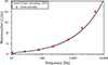 |
Figure 3. Comparison of the dispersion curves of a laminated panel: present methodology (–), model in Ghinet and Atalla [37]. |
Figure 4 compares the modal density predicted by the WFE-SEA method with experimental data from Zhou and Crocker [40]. The evaluated panel comprises a layered sandwich structure with a core (Material IV) and face sheets (Material III), and dimensions Lx = 1.12 m, Ly = 0.62 m, Lz = 7.35 mm. The WFE-SEA model shows very close agreement with the measured data, with a maximum discrepancy of only 2.1%. This discrepancy is likely due to transverse shear deformation effects within the layered structure, which become more prominent at higher frequencies. The WFE model accounts for these effects, whereas simpler reference models may assume classical plate behavior, leading to minor differences.
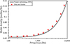 |
Figure 4. Comparison of the modal density of a layered panel: present methodology (–), experimental results in Zhou and Crocker [40]. |
Figure 5 compares the radiation efficiency obtained using the WFE-SEA method with that reported by Yu and Hopkins [42] for a laminated plate of size Lx = 1.62 m, Ly = 1.0 m, Lz = 6.0 mm made from Material V. The results show good agreement across thefrequency range, with minor discrepancies around the coincidence frequency (∼2500 Hz), where even small differences in wave speed or structural damping can lead to larger errors. The discrepancy is limited to approximately 9.7% near the coincidence region, and less than 5% elsewhere, aligning with typical tolerances for SEA-based models near resonance.
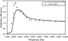 |
Figure 5. Comparison of the radiation efficiency of a laminated plate: present methodology (–), model in Yu and Hopkins [42]. |
Figure 6 presents the STL results from the WFE-SEA model compared against experimental measurements by Zhou and Crocker [40] for the same structure used in the modal density validation. The model accurately reproduces the STL behavior in both sub-coincidence and coincidence regions. A deviation of up to 9.8% is observed at higher frequencies above coincidence, which is attributed to increased structural deflections and damping-related energy dissipation effects that are not fully captured in the analytical approximations used in the referencedata.
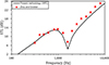 |
Figure 6. Comparison of the sound transmission loss (STL) of a layered panel: present methodology (–), experimental results in Zhou and Crocker [40]. |
Across all comparisons, the WFE-SEA model demonstrates high predictive accuracy, with discrepancies remaining within acceptable bounds (< 10%) for SEA modeling applications. The strong agreement with both numerical and experimental data confirms the method’s robustness and validates its use in analyzing the more complex effects of pre-stress and surface pressure in subsequent sections.
4.2. Impact of tensile pre-stress load on dispersion and vibroacoustic responses
Figures 7 and 8 present the dispersion characteristics and vibroacoustic behavior of the laminated composite panel under varying tensile pre-stress loads.
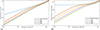 |
Figure 7. Effect of tensile pre-stress on (a) wave dispersion wavenumber and (b) modal density of the laminated panel. |
 |
Figure 8. Vibroacoustic response of the laminated panel under varying tensile pre-stress: (a) acoustic radiation efficiency and (b) sound transmission loss. |
As shown in 7a, increasing the tensile pre-stress load reduces the wavenumber associated with the fundamental antisymmetric Lamb wave mode (A0 mode), resulting in a downward shift in the dispersion curves. This trend indicates that wave propagation becomes less dispersive under tension, which is consistent with the increase in axial stiffness. The wavenumber reduction is inversely related to the magnitude of the applied tensile load. This relationship arises from the positive-definite nature of the geometric stiffness matrix Ks under tensile loading, which effectively enhances the structure’s in-plane rigidity [24]. The corresponding reduction in modal density, shown in 7b, reflects the same stiffening trend. As the structure becomes stiffer, fewer modes are excited within a given frequency range, resulting in lower modal density. This reduction is particularly important in vibroacoustic applications, as it directly influences the amount of structural energy available for acoustic radiation.
Figures 8a and 8b illustrate how tensile pre-stress affects acoustic radiation efficiency and sound transmission loss (STL), respectively. A key observation is the significant leftward shift of the coincidence frequency with increasing tensile load. The peak radiation efficiency occurs at progressively lower frequencies as the pre-stress increases: 15.2 kHz (0 N), 13.6 kHz (20 N), 11.4 kHz (40 N), 9.6 kHz (60 N), 7.6 kHz (80 N), and 5.1 kHz (100 N). This trend indicates that tensile pre-stress reduces the structural wave speeds to the point where they match the airborne sound speed at lower frequencies, thus shifting the coincidence effect earlier in the spectrum. Moreover, the magnitude of the peak radiation efficiency also increases with higher tensile loads, indicating that although coincidence occurs earlier, the structure becomes more acoustically responsive near this transition point.
The STL behavior in Figure 8b follows a similar pattern: as tensile pre-stress increases, the coincidence dip shifts toward lower frequencies, and the STL magnitude reduces in the mid-frequency range. This is especially evident between 5–15 kHz, where the stiffening-induced shift reduces the transmission barrier earlier in the frequency spectrum. However, at higher frequencies (above 100 kHz), the influence of pre-stress diminishes, and STL curves converge, suggesting that tensile effects are more dominant in the low-to-mid frequency regime. The observed vibroacoustic behavior under tensile pre-stress is a direct result of the modifications induced by K s . This in-plane geometric stiffness alters both the modal distribution and wave propagation paths, reducing modal density and reshaping the energy coupling characteristics of the structure. The STL reduction at lower frequencies, while potentially undesirable in passive noise, offers insights into how mechanical pre-conditioning can be used to tune structural-acoustic performance, especially when dynamic loading or adaptive materials areconsidered.
These trends are further confirmed in the 3D visualization presented in Section 4.6, which maps STL variation over frequency and tensile pre-stress. The surface plot clearly illustrates the progressive leftward shift in the STL dip and the reduction in STL magnitude in the coincidence region as tensile load increases.
4.3. Impact of compressive pre-stress load on dispersion and vibroacoustic responses
Figures 9 and 10 illustrate the effect of compressive pre-stress on wave dispersion and vibroacoustic performance of the laminated composite.
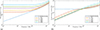 |
Figure 9. Effect of compressive pre-stress on wave characteristics of the laminated panel: (a) dispersion wavenumber and (b) modal density. |
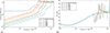 |
Figure 10. Effect of compressive pre-stress on (a) acoustic radiation efficiency and (b) sound transmission loss of the laminated panel. |
As shown in Figure 9a, compressive pre-stress increases the dispersion wavenumber of the A0 mode. This enhancement in wave dispersion is attributed to the negative real-valued stiffness contribution of Ks under compression, which effectively softens the in-plane response [24]. Correspondingly, the modal density (Fig. 9b) increases with higher compressive load, especially above 100 kHz, where wave-structure interactions are more sensitive to changes in stiffness. Below 100 kHz, the behavior is nearly symmetric to that under tensile stress due to similar strain energy magnitudes.
Compressive loading shifts the coincidence frequency to higher values, as seen in Figure 10a. Peak radiation efficiency occurs at 15.2 kHz (0 N), increasing to 108.5 kHz (400 N), indicating a delay in acoustic coupling due to structural softening. At lower frequencies, radiation efficiency decreases with increased compression, while convergence is observed at high frequencies. Similarly, Figure 10b shows a rightward shift in the STL coincidence dip with increasing compressive stress, contrasting the downward trend observed under tension. This behavior is driven by an increase in modal density and wave dispersion due to the softening of in-plane wave modes under compression. As more modes become active at higher frequencies, acoustic coupling is delayed, resulting in a higher coincidence frequency. Additionally, the STL magnitude slightly decreases in the mid-frequency range as energy is distributed across a broader modal spectrum. At high frequencies, the STL responses converge, suggesting that the influence of compressive loading diminishes relative to modal saturation effects.
These results demonstrate that compressive pre-stress modifies the structure’s vibroacoustic response primarily by shifting modal participation and wave propagation characteristics. The influence of Ks under compression is opposite to that of tension, resulting in higher modal density and delayed coincidence effects, as further illustrated in Figure 15b
4.4. Impact of surface pressure load on dispersion and vibroacoustic responses
Figures 11 and 12 illustrate the influence of surface pressure loading on the laminated panel’s dispersion characteristics and vibroacoustic performance.
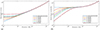 |
Figure 11. Effect of surface pressure load on (a) wave dispersion wavenumber and (b) modal density of the laminated panel. |
 |
Figure 12. Effect of surface pressure load on (a) acoustic radiation efficiency and (b) sound transmission loss of the laminated panel. |
As shown in Figure 11a, surface pressure increases the dispersion wavenumber at low frequencies, indicating a stiffer out-of-plane response. This is attributed to the contribution of the pressure-induced stiffness matrix KP, which enhances bending resistance across the panel. Concurrently, the modal density (Fig. 11b) decreases with increasing pressure, particularly below 100 kHz, due to the reduced number of accessible modes in the stiffened system. At higher frequencies, the influence of pressure diminishes, and both wavenumber and modal density trends converge. This is because, as frequency increases, the contribution of pressure-induced stiffness becomes relatively less significant compared to the overall modal excitation, leading to convergence in the panel’s response.
Figure 12a shows that increasing surface pressure leads to a decrease in radiation efficiency before the coincidence frequency (∼15.2 kHz). This reduction stems from delayed mode coupling, as the pressurized structure resists out-of-plane acoustic excitation more effectively. Beyond the coincidence frequency, radiationefficiency levels out across pressure levels. STL results in Figure 12b show overall similarity across pressure levels, with a key difference being the rightward shift in the coincidence dip. The coincidence frequency rises from 12 kHz under 0.6 GPa to 20 kHz in the unpressurized condition, reflecting the stiffer bending response induced by K P . However, the STL magnitude remains nearly constant outside this region.
Surface pressure modifies the panel’s vibroacoustic response primarily through out-of-plane stiffening, captured by K P , which shifts wave propagation and coupling behavior without significantly altering broadband STL levels. This trend is further visualized through a STL surface plot presented in Section 4.6, confirming the frequency shift and slight STL suppression near coincidence.
4.5. Impact of pre-stress and surface pressure loads on dispersion and vibroacoustic responses
Figures 13 and 14 illustrate the effects of combined tensile pre-stress and surface pressure loads on the wave propagation and vibroacoustic behavior of the laminated composite panel.
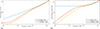 |
Figure 13. Effect of combined tensile pre-stress and surface pressure on (a) wave dispersion wavenumber and (b) modal density of the laminated panel. |
 |
Figure 14. Effect of combined tensile pre-stress and surface pressure on (a) acoustic radiation efficiency and (b) sound transmission loss of the laminated panel. |
Figure 13a shows that the dispersion wavenumber under combined loading lies between those for individual pre-stress and pressure cases. For example, at 100 Hz, the wavenumber is 4.5 m−1 under 50 N pre-stress, 35 m−1 under 0.02 GPa pressure, and 10.1 m−1 under the combined loading – indicating that pressure has a stronger influence on wave dispersion. A similar trend is observed in the modal density (Fig 13b), where the value under combined loading (0.0018 at 100 Hz) falls between that for pressure (0.011) and pre-stress alone (0.0012), confirming the dominant stiffening role of KP in the combined condition.
Radiation efficiency under combined loading decreases compared to pressure-only cases, with a lower peak magnitude and earlier coincidence frequency. As shown in Figure 14a, the peak efficiency is 5.8 at 10.2 kHz under combined 50 N pre-stress and 0.02 GPa pressure, compared to 46.4 at 12.5 kHz under pressure alone. This reduction aligns closely with the behavior under pre-stress-only loading, suggesting that the directional influence of Ks counteracts some of the stiffening effects from KP, thereby shifting the acoustic coupling region earlier. The STL results in Figure 14b support this observation. The coincidence dip under combined loading shifts to lower frequencies than in the pressure-only case, resulting in STL performance more similar to that ofpre-stressed panels. While pressure elevates bending stiffness, the directional modulation introduced by pre-stress reduces the net radiative response in key frequency bands.
Combined loading introduces a nuanced interaction between out-of-plane stiffening from KP and directional in-plane effects from Ks. The resulting vibroacoustic response is not simply additive but reflects a superposition of opposing influences, with pre-stress modifying the effective contribution of surface pressure. This dynamic is further visualized in Figure 15d, where STL dips shift in both magnitude and frequency in response to combined loading conditions.
4.6. STL visualization and interpretation of stiffness contributions
To enhance the interpretability of the sound transmission loss (STL) trends under different loading conditions, additional visualizations and comparative stiffness analysis have been included in this section. Figures 15a–15d illustrate STL as a function of frequency and various mechanical loading conditions.
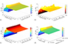 |
Figure 15. STL as a function of frequency and various mechanical loading conditions: (a) tensile pre-stress, (b) compressive pre-stress, (c) surface pressure, and (d) combined pre-stress and pressure. |
Figure 15a presents STL variations under tensile pre-stress loading. As pre-stress increases from 0 to 60 N, the coincidence frequency clearly shifts to lower frequencies, with a corresponding decrease in STL in the low-frequency band (0.1–3 kHz). At higher frequencies, STL gradually recovers due to flexural stiffening induced by the axial load. Figure 15b illustrates STL behavior under compressive pre-stress. The STL response is initially flat but begins to exhibit nonlinear changes beyond 100 N, especially at higher frequencies, where certain frequencies show slight STL enhancement or dips, indicating a complex redistribution of modal energy due to compressive effects on in-plane stiffness.
Figure 15c shows STL as a function of surface pressure, ranging from 0 to 0.6 GPa. At lower frequencies, STL remains almost constant across pressure levels. However, in the mid-frequency range (10–40 kHz), STL tends to decrease slightly with increasing pressure, suggesting that surface pressure raises the panel’s out-of-plane stiffness, altering wave propagation paths and reducing energy dissipation. Figure 15d captures the combined effect of pre-stress and pressure. The interaction between the two loading types results in a more nuanced STL response: STL increases initially under moderate loading but then drops significantly in certain frequency bands (8–20 kHz) due to competing effects between in-plane tension and surface pressure.
These plots demonstrate that STL behavior is strongly frequency-dependent and load-sensitive, especially around modal transition zones and the coincidence region. They also highlight how tuning loading conditions could be leveraged to tailor STL characteristics in structural design.
To provide a deeper understanding of the physical mechanisms underlying these STL changes, the discussion is expanded role of the stiffness matrices, as follows:
Pre-stress-induced stiffness K S arises from in-plane axial or biaxial loading. It introduces direction-dependent stiffness variations, influencing in-plane wave speeds and causing secondary effects on out-of-plane flexural wave propagation. This explains the frequency shifting and localized STL reduction seen with tensile and compressive pre-stress. When normalized by the baseline stiffness K 0 , results indicate that for pre-stress around 50–100 N, K S contributes about 10–15%, but with a stronger directional bias.
Pressure-induced stiffness K P results from normal surface pressure acting uniformly across the panel. It affects the out-of-plane deformation resistance, increasing the structure’s flexural rigidity. This leads to modest STL attenuation at mid-frequencies, as the panel becomes less compliant and radiative modes are altered. When normalized by the baseline stiffness K 0 , results indicate that at moderate pressure (e.g., 0.2–0.4 GPa), K P contributes approximately 20–25% to the total stiffness, concentrated in transverse degrees of freedom.
These contributions explain the nonlinear and anisotropic nature of STL trends observed under varying mechanical loads.
5. Conclusion
This study has presented a detailed numericalinvestigation into the effects of tensile pre-stress, compressive pre-stress, and surface pressure loads on the vibroacoustic performance of laminated composite panels using a Wave Finite Element (WFE)-based Statistical Energy Analysis (SEA) framework. The methodology enables the evaluation of frequency-dependent wave propagation and vibroacoustic metrics, including modal density, radiation efficiency, and sound transmission loss (STL), across a broad frequency range and under varying mechanical loading conditions.
The modeling approach was validated against benchmark experimental and numerical results from the literature. Excellent agreement was achieved for wavedispersion, modal density, radiation efficiency, and STL, with discrepancies remaining below 10%, thereby confirming the reliability of the proposed WFE-SEA framework for layered composite structures.
Key findings from the numerical analysis include:
-
(a)
Tensile pre-stress reduces both dispersion and modal density due to increased in-plane stiffness KS. For instance, at 100 Hz, the wavenumber and modal density decreased to 4.5 m−1 and 0.0012, respectively, under a 50 N tensile load. This results in a lower coincidence frequency, shifting from 15.2 kHz (no load) to 5.1 kHz (100 N) in radiation efficiency, and correspondingly in STL.
-
(b)
Compressive pre-stress shows the inverse behavior, increasing dispersion and modal density. The coincidence frequency in STL increases from 15.2 kHz (0 N) to 108.5 kHz (400 N), reflecting delayed acoustic coupling and reduced low-frequency radiation efficiency.
-
(c)
Surface pressure loading primarily affects out-of-plane stiffness KP. At 0.02 GPa pressure, the wavenumber at 100 Hz reaches 35 m−1, and modal density reaches 0.011, significantly higher than under pre-stress alone. Coincidence frequency shifts from 20 kHz (0 GPa) to 12 kHz (0.6 GPa) in STL, showing earlier radiation onset.
-
(d)
Combined loading produces an intermediate dynamic response. For instance, at 100 Hz, the wavenumber and modal density under 50 N + 0.02 GPa are 10.1 m−1 and 0.0018, respectively, falling between their individual load counterparts. Radiation efficiency peaks at 10.2 kHz, closer to the pre-stress response than pressure-only behavior, indicating dominant in-plane modulation by KS.
The study demonstrates that both pre-stress and surface pressure significantly influence wave propagation and acoustic energy transmission. These effects are governed by the relative contributions of the in-plane K S and out-of-plane K P stiffness matrices. The findings provide actionable insights for tuning the acoustic response of laminated composites through controlled loading conditions, with relevance for aerospace, transport, and high-precision structural applications.
Fundings
This work was partly supported by the following grants: BJIM Matching Grant (Grant No.: 1001. PMEKANIK. 8070022) and USM-WD CiA Lab Grant (Grant No.: 311/PMEKANIK/4402055).
Conflicts of interest
The author(s) declared no potential conflicts of interest with respect to the research, authorship, and/or publication of this article.
Data availability statement
Data are available on request from the authors.
Author contribution statement
Rilwan Kayode Apalowo: Conceptualization, Formal analysis, Investigation, Methodology, Validation, Visualization, Writing – original draft, Writing – revised draft, Aizat Abas: Conceptualization, Investigation, Methodology, Validation, Funding acquisition, Supervision; Dimitrios Chronopoulos: Conceptualization, Investigation, Methodology, Validation, Supervision.
References
- J. Fan, J. Njuguna: An introduction to lightweight composite materials and their use in transport structures, in: Lightweight Composite Structures in Transport: Design, Manufacturing, Analysis and Performance. Woodhead Publishing, 2016, pp. 3–34. [Google Scholar]
- M. Girardi, C. Padovani, D. Pellegrini, L. Robol: A finite element model updating method based on global optimization. Mechanical Systems and Signal Processing 152 (2021) 107372. [Google Scholar]
- D. Chronopoulos, B. Troclet, M. Ichchou, J.P. Lainé: A unified approach for the broadband vibroacoustic response of composite shells. Composites Part B: Engineering 43 (2012) 1837–1846. [Google Scholar]
- R.K. Apalowo, D. Chronopoulos, M. Malik: The influence of temperature on wave scattering of damaged segments within composite structures. MATEC Web of Conferences 211 (2018) 19005. [Google Scholar]
- H. Zhang, Z. Li, Y. Deng, H. Li, H. Cao, X. Wang: Optimal design study of vibro-acoustic resistance of porous foam composite laminates. Applied Composite Materials 31 (2024) 1663–1686. [Google Scholar]
- D. Zheng, W.K. Binienda: Analysis of impact response of composite laminates under prestress. Journal of Aerospace Engineering 21 (2008) 197–205. [Google Scholar]
- H. Saghafi, T. Brugo, A. Zucchelli, C. Fragassa, G. Minak: Comparison of the effect of preload and curvature of composite laminate under impact loading. FME Transactions 44 (2016) 353. https://search.ebscohost.com/login.aspx?direct=true&profile=ehost&scope=site&authtype=crawler&jrnl=14512092&AN=120724552&h=v7kX9KIVcE%2F0nT%2FFYtxzW1f5MjRxNAGVJFocwMerqRZACNNE2AoZIPNrwbSPvCWF3yUQ6Pyic3htqVWbcE9%2F%2FQ%3D%3D&crl=c (accessed March 13, 2025). [Google Scholar]
- A. Tarkashvand, M. Montasheri, K. Daneshjou: Analysis of vibroacoustic behavior of partially coupled fluid-structure laminated composite cylinders using two coordinate systems. Ocean Engineering 292 (2024) 116525. [Google Scholar]
- Z. Shen, R. Dong, J. Li, Y. Su, X. Long: Determination of gradient residual stress for elastoplastic materials by nanoindentation. Journal of Manufacturing Processes 109 (2024) 359–366. [Google Scholar]
- W. Zhang, J. Huang, J. Lin, B. Lin, X. Yang, Y. Huan: Experimental and numerical investigation of mechanical behavior of segmental joint of shield tunneling strengthened by prestressed CFRP plates. Structures 70 (2024) 107634. [Google Scholar]
- Y. Wang, Z. Han, X. Xu, Y. Luo: Topology optimization of active tensegrity structures. Computers & Structures 305 (2024) 107513. [Google Scholar]
- X. Mi, Y. Zhao, Q. Zhan, M. Chen: Vibration reduction study of a simplified floating raft system by installing connecting nonlinear spring-mass systems. Thin-Walled Structures 210 (2025) 113015. [Google Scholar]
- R.K. Apalowo, D. Chronopoulos: Vibroacoustic design optimization of curved composite shells. Polymers and Polymer Composites 29 (2021) S1520–S1531. [Google Scholar]
- R.K. Apalowo, D. Chronopoulos, S. Cantero-Chinchilla: Wave interaction with nonlinear damage and generation of harmonics in composite structures. Composite Structures 230 (2019) 111495. [Google Scholar]
- S. Ghinet, N. Atalla, H. Osman: The transmission loss of curved laminates and sandwich composite panels. Journal of the Acoustical Society of America 118 (2005) 774–790. [Google Scholar]
- S. Ghinet, N. Atalla, H. Osman: Diffuse field transmission into infinite sandwich composite and laminate composite cylinders. Journal of Sound and Vibration 289 (2006) 745–778. [Google Scholar]
- Y. Yang, M. Kingan: A hybrid wave and finite element/boundary element method for predicting the vibroacoustic characteristics of finite-width complex structures. Journal of Sound and Vibration 582 (2024) 118402. [Google Scholar]
- B. Zaparoli Cunha, C. Droz, A.M. Zine, S. Foulard, M. Ichchou: A review of machine learning methods applied to structural dynamics and vibroacoustic. Mechanical Systems and Signal Processing 200 (2023) 110535. [Google Scholar]
- N. Gao, M. Wang, X. Liang, G. Pan: On-demand prediction of low-frequency average sound absorption coefficient of underwater coating using machine learning. Results in Engineering 25 (2025) 104163. [Google Scholar]
- S. Wang, J. He, J. Fan, P. Sun, D. Wang: A time-domain method for free vibration responses of an equivalent viscous damped system based on a complex damping model. Journal of Low Frequency Noise Vibration and Active Control 42 (2023) 1531–1540. [Google Scholar]
- N. Gao, H. Yu, J. Liu, J. Deng, Q. Huang, D. Chen, G. Pan: Experimental investigation of composite metamaterial for underwater sound absorption. Applied Acoustics 211 (2023) 109466. [Google Scholar]
- F. Liu, X. Zhao, Z. Zhu, Z. Zhai, Y. Liu: Dual-microphone active noise cancellation paved with Doppler assimilation for TADS. Mechanical Systems and Signal Processing 184 (2023) 109727. [Google Scholar]
- B.R. Mace, E. Manconi: Modelling wave propagation in two-dimensional structures using finite element analysis. Journal of Sound and Vibration 318 (2008) 884–902. [Google Scholar]
- E. Manconi, B.R. MacE, R. Garziera: The loss-factor of pre-stressed laminated curved panels and cylinders using a wave and finite element method. Journal of Sound and Vibration 332 (2013) 1704–1711. [Google Scholar]
- N. Aimakov, G. Tanner, D. Chronopoulos: A wave finite element approach for modelling wave transmission through laminated plate junctions. Scientific Reports 12, 1 (2022) 1–15. [CrossRef] [PubMed] [Google Scholar]
- D. Chronopoulos, C. Droz, R. Apalowo, M. Ichchou, W.J. Yan: Accurate structural identification for layered composite structures, through a wave and finite element scheme. Composite Structures 182 (2017) 566–578. [Google Scholar]
- T. Ampatzidis, D. Chronopoulos: Acoustic transmission properties of pressurised and pre-stressed composite structures. Composite Structures 152 (2016) 900–912. [Google Scholar]
- C. Fenemore, M.J. Kingan, B.R. Mace: Application of the wave and finite element method to predict the acoustic performance of double-leaf cross-laminated timber panels. Building Acoustics 30 (2023) 203–225. [Google Scholar]
- M.R. Zarastvand, M. Ghassabi, R. Talebitooti: Prediction of acoustic wave transmission features of the multilayered plate constructions: a review. Journal of Sandwich Structures and Materials 24 (2022) 218–293. [Google Scholar]
- Y. Luo, X. Zhang, H. Zhou, L. Elmaimouni: Shear horizontal wave propagation in piezoelectric semiconductor nanoplates with the consideration of surface effects and nonlocal effects. Mechanics of Advanced Materials and Structures (2025). https://doi.org/10.1080/15376494.2025.2488058. [Google Scholar]
- P. Zhang, W. Shao, H. Arvin, W. Chen, W. Wu: Nonlinear free vibrations of a nanocomposite micropipes conveying laminar flow subjected to thermal ambient:employing invariant manifold approach. Journal of Fluids and Structures 135 (2025) 104311. [Google Scholar]
- Y. Yang, C. Fenemore, M.J. Kingan, B.R. Mace: Analysis of the vibroacoustic characteristics of cross laminated timber panels using a wave and finite element method. Journal of Sound and Vibration 494 (2021) 115842. [Google Scholar]
- E. Manconi, B.R. Mace, R. Garziera: Wave propagation in laminated cylinders with internal fluid and residual stress. Applied Sciences 13 (2023) 5227. [Google Scholar]
- Y. Yang, B.R. Mace, M.J. Kingan: Prediction of sound transmission through, and radiation from, panels using a wave and finite element method. The Journal of the Acoustical Society of America 141 (2017) 2452–2460. [Google Scholar]
- V. Cool, R. Boukadia, L. Van Belle, W. Desmet, E. Deckers: Contribution of the wave modes to the sound transmission loss of inhomogeneous periodic structures using a wave and finite element based approach. Journal of Sound and Vibration 537 (2022) 117183. [Google Scholar]
- V. Cotoni, R.S. Langley, P.J. Shorter: A statistical energy analysis subsystem formulation using finite element and periodic structure theory. Journal of Sound and Vibration 318 (2008) 1077–1108. [Google Scholar]
- S. Ghinet, N. Atalla: Vibro-acoustic behaviour of flat sandwich composite panels. Transactions of The Canadian Society for Mechanical Engineering 30 (2006) 473–493. [Google Scholar]
- F.G. Leppington, E.G. Broadbent, K.H. Heron: The acoustic radiation efficiency of rectangular panels. Proceedings of the Royal Society of London. A. Mathematical and Physical Sciences 382 (1982) 245–271. [Google Scholar]
- F.G. Leppington, K.H. Heron, E.G. Broadbent: Resonant and non-resonant transmission of random noise through complex plates. Proceedings of the Royal Society of London. Series A: Mathematical, Physical and Engineering Sciences 458 (2002) 683–704. [Google Scholar]
- R. Zhou, M.J. Crocker: Sound transmission loss of foam-filled honeycomb sandwich panels using statistical energy analysis and theoretical and measured dynamic properties. Journal Of Sound And Vibration 329 (2010)673–686. [Google Scholar]
- J.F. Allard, N. Atalla: Propagation of Sound in Porous Media: Modelling Sound Absorbing Materials, Propagation of Sound in Porous Media: Modelling Sound Absorbing Materials (2009) 1–358. [Google Scholar]
- Y. Yu, C. Hopkins: Reduced order integration for the radiation efficiency of a rectangular plate. JASA Express Letters 1 (2021) 062801. [Google Scholar]
Cite this article as: Apalowo R.K. Abas A. & Chronopoulos D. 2025. Impacts of pressure and pre-stress loads on the vibroacoustic response of laminated composite structures. Acta Acustica, 9, 52. https://doi.org/10.1051/aacus/2025036.
All Tables
All Figures
|
Figure 1. Configuration of a laminated composite under pressure and pre-stress (compression) loads. |
| In the text | |
|
Figure 2. Schematic representation of acoustic transmission in the statistical energy analysis context. |
| In the text | |
|
Figure 3. Comparison of the dispersion curves of a laminated panel: present methodology (–), model in Ghinet and Atalla [37]. |
| In the text | |
|
Figure 4. Comparison of the modal density of a layered panel: present methodology (–), experimental results in Zhou and Crocker [40]. |
| In the text | |
|
Figure 5. Comparison of the radiation efficiency of a laminated plate: present methodology (–), model in Yu and Hopkins [42]. |
| In the text | |
|
Figure 6. Comparison of the sound transmission loss (STL) of a layered panel: present methodology (–), experimental results in Zhou and Crocker [40]. |
| In the text | |
|
Figure 7. Effect of tensile pre-stress on (a) wave dispersion wavenumber and (b) modal density of the laminated panel. |
| In the text | |
|
Figure 8. Vibroacoustic response of the laminated panel under varying tensile pre-stress: (a) acoustic radiation efficiency and (b) sound transmission loss. |
| In the text | |
|
Figure 9. Effect of compressive pre-stress on wave characteristics of the laminated panel: (a) dispersion wavenumber and (b) modal density. |
| In the text | |
|
Figure 10. Effect of compressive pre-stress on (a) acoustic radiation efficiency and (b) sound transmission loss of the laminated panel. |
| In the text | |
|
Figure 11. Effect of surface pressure load on (a) wave dispersion wavenumber and (b) modal density of the laminated panel. |
| In the text | |
|
Figure 12. Effect of surface pressure load on (a) acoustic radiation efficiency and (b) sound transmission loss of the laminated panel. |
| In the text | |
|
Figure 13. Effect of combined tensile pre-stress and surface pressure on (a) wave dispersion wavenumber and (b) modal density of the laminated panel. |
| In the text | |
|
Figure 14. Effect of combined tensile pre-stress and surface pressure on (a) acoustic radiation efficiency and (b) sound transmission loss of the laminated panel. |
| In the text | |
|
Figure 15. STL as a function of frequency and various mechanical loading conditions: (a) tensile pre-stress, (b) compressive pre-stress, (c) surface pressure, and (d) combined pre-stress and pressure. |
| In the text | |
Current usage metrics show cumulative count of Article Views (full-text article views including HTML views, PDF and ePub downloads, according to the available data) and Abstracts Views on Vision4Press platform.
Data correspond to usage on the plateform after 2015. The current usage metrics is available 48-96 hours after online publication and is updated daily on week days.
Initial download of the metrics may take a while.