


| Issue |
Acta Acust.
Volume 10, 2026
Topical Issue - Proceedings of AFPAC 2026
|
|
|---|---|---|
| Article Number | 71 | |
| Number of page(s) | 14 | |
| DOI | https://doi.org/10.1051/aacus/2026069 | |
| Published online | 03 August 2026 | |
Scientific Article
Improving defect detection of nuclear welds using adaptive imaging based on uncertain material parameters optimization
Université Paris-Saclay, CEA, List, F-91120 Palaiseau, France
* Corresponding author: This email address is being protected from spambots. You need JavaScript enabled to view it.
Received:
31
March
2026
Accepted:
29
June
2026
Abstract
Weld inspection in the nuclear sector is crucial for ensuring the structural integrity and safety of reactor cooling piping systems. Given the strict safety requirements, reliable and accurate Non-Destructive Evaluation (NDE) techniques are essential for the early detection and characterisation of defects. In this context, phased-array ultrasonic imaging has emerged as a powerful tool for advanced NDE. Among these techniques, the Total Focusing Method (TFM) with Full Matrix Capture (FMC) is widely recognised for its superior signal-to-noise ratio and imaging performance. Weld inspection remains challenging due to the anisotropic and heterogeneous nature of weld microstructures, which distort wavefronts, increase structural noise, and are often only imprecisely characterised. This work addresses the latter issue, as TFM images become distorted when the Time of Flight (ToF) used for reconstruction deviates from the physical ToF. Correcting the ToF is therefore necessary to compensate for these aberrations. This study enhances an existing adaptive imaging approach based on TFM, the use of a complex weld model, and the optimisation of an imaging criterion within the space of the weld model parameters. Unlike the initial version, which required prior knowledge of defect locations, the enhanced framework automatically identifies subzones with a high likelihood of containing defects. An improved global normalised criterion is then applied to enhance image quality. A more robust hybrid optimiser, combining global exploration and local refinement, is employed, improving both stability and computational efficiency. The approach was validated using experimental and simulated FMC datasets, demonstrating improved defect detectability and image quality, and was implemented as a CIVA plugin.
Key words: NDE / Ultrasound imaging / TFM / Weld / Optimisation
© The Author(s), Published by EDP Sciences, 2026
 This is an Open Access article distributed under the terms of the Creative Commons Attribution License (https://creativecommons.org/licenses/by/4.0), which permits unrestricted use, distribution, and reproduction in any medium, provided the original work is properly cited.
1 Introduction
In the nuclear sector, where safety is paramount, the inspection of welded assemblies is essential to ensure reactor reliability. Phased-array ultrasonic imaging methods are increasingly used to inspect these structures, enabling the detection and sizing of defects, particularly near weld bevels and within heat-affected zones, where cracks induced by thermal fatigue or corrosion commonly initiate and propagate over time. Several ultrasonic imaging techniques have been developed and reported in the literature for both medical and NDE applications. Among these, the Total Focusing Method (TFM), Plane Wave Imaging (PWI), and Phase Coherence Imaging (PCI) have demonstrated high performance in terms of defect detectability and signal-to-noise ratio (SNR) [1–5]. However, these techniques require prior knowledge of the material properties to compute the ToF required for image reconstruction. This requirement poses a significant challenge, particularly in the case of heterogeneous and anisotropic welds. The microstructural properties of such welds are generally unknown and may vary from one weld to another. This variability arises from environmental conditions and operator-dependent factors inherent to the welding process.
In weld inspection, defects located before the weld generally have a limited impact on the TFM image. This is because the useful information carried by the reflected ultrasonic waves primarily originates from propagation through the base metal, whose material properties are well known. In contrast, defects located within or beyond the weld are significantly more challenging to detect, as the anisotropic and heterogeneous elastic properties of the weld distort wave paths, affecting both image quality and defect detectability. These imaging challenges arise from amplitude losses caused by grain scattering of the coherent wavefront, backscattering noise, and spatial variations in grain orientation, which induce significant phase velocity variations. While scattering and noise are difficult to compensate for, phase aberrations induced by wavefront distortions can, in principle, be mitigated if an accurate and representative weld model is available. Assuming the weld to be homogeneous and isotropic introduces significant errors in the estimated ToF, leading to distortions in the reconstructed TFM image. This underscores the need to correct ToF calculations using representative weld models that account for anisotropy and heterogeneity. Several approaches have been proposed in the literature to invert both the stiffness properties of welds and the grain orientations associated with the symmetry axis of transverse isotropy of the effective material. Three main families of methods have been developed.
The first family of approaches is based on machine learning and deep learning frameworks. A machine learning framework was developed in [6], enhanced with a diffusion-based distribution, to automate weld inspection using elastic guided waves, enabling surface crack identification and weld stiffness estimation. The training dataset was generated using a hierarchical simulation scheme. In [7], a deep learning framework was developed to invert the fibre orientation of an austenitic weld using travel-time data for each emitter–receiver pair. In this study, the stiffness was assumed to be known, and the data were generated using an Ogilvy-type representation of the weld with local perturbations. A variant of the fast marching method adapted to anisotropic materials was employed to compute ToFs, and validation was performed using data generated from high-fidelity finite element simulations. Although these approaches have demonstrated promising performance for industrial applications, they remain constrained by the simplified cases used to generate the training datasets and are associated with high computational costs during the training phase.
The second family comprises optimisation-based approaches that aim to minimise a cost function in order to invert weld material properties. In [8], an optimisation method was developed to invert the distribution of grain orientations based on an Ogilvy-type model, with random perturbations introduced to increase the complexity of the weld description. The discrepancy between measured times of arrival of reflectors extracted from the FMC matrix and simulated times of arrival computed using the fast marching method was minimised. An evolution strategy was employed as a global optimiser. The resulting inverted orientation map was subsequently used to generate TFM images, leading to improved defect detectability in welds. Similarly, in [9], a multi-objective function based on the spatial positions of echoes with maximum amplitude under different configurations was minimised to invert weld orientations. The weld was modelled as a collection of homogeneous transversely isotropic subdomains, and ToF values were computed using a fast marching algorithm. In [10], an optimisation-based inversion of weld orientation maps was proposed using ultrasonic tomography combined with a nonlinear conjugate gradient optimiser. The cost function was defined as the sum of squared errors between experimental and simulated ToF values for each transmitter–receiver pair. A new forward model, referred to as the shortest ray path model, was introduced. The weld orientation map was discretised on a grid, with each cell assigned an orientation angle while sharing identical crystal stiffness properties expressed in the local coordinate system. To facilitate convergence, an Ogilvy map was used as an initial guess, and regularisation terms were incorporated into the cost function.
The third family consists of probabilistic approaches. In [11], the authors proposed a probabilistic inversion framework based on ultrasonic tomography to estimate both the orientation and stiffness of a heterogeneous anisotropic layer. To reduce the number of stiffness parameters, the transversely isotropic stiffness tensor was parameterised using two scalar quantities, scale and strength, defined relative to reference isotropic and anisotropic stiffness tensors. The probabilistic inversion was formulated within a variational Bayesian framework using stochastic Stein variational gradient descent, which aims to approximate the posterior distribution by incorporating prior knowledge of the parameters and a forward model to compute the ToF values used in the likelihood distribution. Similarly, [12] proposed an approach based on a reversible-jump Markov Chain Monte Carlo method to approximate the posterior distribution. In their framework, the weld orientation map was parameterised using a Voronoi tessellation, where both the number and geometry of the Voronoi cells, as well as the orientation assigned to each cell, were allowed to vary. However, the stiffness parameters were assumed to be known and fixed. In the same study, a novel fast marching algorithm, referred to as the *anisotropic multi-stencil fast marching method*, was introduced to efficiently handle wave propagation in anisotropic and heterogeneous materials such as welds.
Most of the existing approaches have focused primarily on inverting the fibre texture orientation and stiffness properties of heterogeneous anisotropic materials, such as welds. While these methods have demonstrated promising results for future industrial applications, an alternative strategy is to focus on improving the quality of the ultrasonic image itself, rather than precisely estimating weld orientation and stiffness. In [13, 14], the original approach consisted of optimising an imaging criterion that maximises the amplitude of potentially coherent signals in order to enhance the quality of TFM images compared to current industrial practices, which rely on simpler material models assumed to be homogeneous and isotropic.
In this method, the weld orientation is also modelled using an Ogilvy-type orientation map, while the material retains transverse isotropic symmetry along the local fibre axis. In addition, ToFs are calculated using a ray-tracing model. The results demonstrated improved TFM image quality in terms of both SNR and defect detectability. Simultaneously, the estimated orientation map and stiffness properties converged towards the reference values. In simulated cases where the weld was fully insonified by the array elements, the most influential parameters were successfully recovered. This approach offers greater flexibility in practical scenarios where the other methods may fail. One limitation of this approach is that it requires reasonably accurate prior knowledge of the defect location.
In the current study, we build on this work by extending the method to eliminate the need for a priori knowledge of defect locations and by introducing a more sophisticated spatial imaging criterion. Additionally, a more robust hybrid optimiser, TikTak [15], was incorporated to replace the particle swarm optimisation algorithm used in the original study [16]. This enhanced approach was implemented as a plugin within the NDE software CIVA [17, 18], developed by the CEA. The proposed method was validated using both simulated and experimental FMC datasets. The article is organised into two sections. In the first section, we briefly present the initial approach proposed by Ménard et al. [13] and, in greater detail, the new developments introduced in the enhanced approach. In the second section, we present the new results, including a comparison with a reference state generated using finite element analysis, as well as results obtained from experimentally acquired FMC data. In the experimental case, the defect positions are known, whereas the weld stiffness and orientation properties are not. In both scenarios, a comparison with the classical assumption of a homogeneous isotropic weld is provided.
2 TFM imaging using adaptive weld-based model
In the approach proposed by Ménard et al. [13], the optimisation criterion is defined as the maximum amplitude of the TFM image, under the assumption that both the global inspected Region of Interest (ROI) and the local ROI containing the defect are known a priori. As previously noted, the weld orientation map is modelled using an Ogilvy-type representation [19], with the weld material assumed to be transversely isotropic. The optimisation is performed using the particle swarm optimisation (PSO) algorithm, as detailed in Algorithm 1 in the Appendix.
In the following sections, we present the optimisation problem addressed in [13] (Sect. 2.1), followed by a description of the weld model (Sect. 2.2) and the forward model used for ToF computation (Sect. 2.3). We then highlight the principal improvements introduced in this work in Section 2.4, concerning the formulation of the optimisation problem, the choice of optimiser, and the automation of the determination of the local ROI within the globally defined inspected ROI. Throughout this section, the methodology description is based on the configuration presented in Figure 1, which corresponds to an L0° inspection of a double-V (double bevel) weld containing three side-drilled holes (SDHs) located along the right bevel. A linear array transducer composed of 128 elements, with a central frequency of 4 MHz, is considered. The same configuration is used in the results section for simulated FMC data. The weld model employed in this study will be described in the following subsections, while the associated parameters will be presented in the Section 3.1.
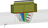 |
Figure 1. Configuration of the simulated FMC. |
2.1 Description of the optimisation problem
Let us consider the 2-D welded assembly (in the (o z x) plane) illustrated in Figure 2. The domains Ω1 and Ω3 denote the base metal regions, while Ω2 represents the weld region. The base metal domains Ω1 and Ω3 are assumed to be isotropic, homogeneous, and characterised by known material properties. In contrast, the weld domain Ω2 is considered heterogeneous and transversely isotropic, with its fibre orientation described by the Ogilvy model (details of the stiffness and orientation modelling are provided in the following sections).
 |
Figure 2. Schematic representation of the three domains Ω1, Ω2, and Ω3, corresponding to the base metal and the weld, together with the global region of interest Ω D (0) and the local region of interest Ω D . |
Let X denote the unknowns describing the weld material properties in Ω2, comprising X stif, which consists of N stif independent stiffness components, and X orient, which represents the N orient orientation map parameters. The objective is to enhance ultrasound imaging through the welded structure by optimising an imaging criterion. The imaging technique used is TFM, and the selected imaging criterion is the maximum amplitude within a local ROI.
Let Ω D (0) be the global ROI enclosing the inspected weld, which is assumed to be known a priori, Ω D ⊂ Ω D (0) be the local ROI containing the defect (see Fig. 2), and 𝒢D denote the discrete imaging grid associated with ΩD. In the following, the TFM imaging operator is denoted by I(X) for a given weld description X. The maximum amplitude functional over the pixels of the imaging grid 𝒢D is defined as:

In [13, Ω D is assumed to be known. The optimisation problem can then be formulated as

the enhanced image being therefore given by I(X *).
2.2 Weld material modelling for ToF corrections
To compute the ToF needed for the construction of the TFM image, the stiffness and orientation properties of the weld must be known in order to solve the Christoffel equation and deduce the slowness values of the chosen mode (corresponding to the quasi-longitudinal mode in this study) along the ray path. The weld material stiffness  was considered transversely isotropic with constant stiffness properties, considering (1, 2) as the plane of isotropy:
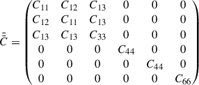
with 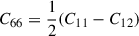 .
.
Thus, the stiffness tensor has 5 independent parameters C 11, C 12, C 13, C 33, C 44. Since we treat only the 2D case, with the assumption of plane strain, the 5 independent parameters reduce to N stif = 4 independent parameters, and thus it follows that:

The weld map orientation θ(x, z), which corresponds to the angle between the z-axis and the local axis of anisotropy (when θ = 0°, the axis of local anisotropy is aligned with the z-axis), was described using the Ogilvy parametric model with N orient = 4 independent parameters (D, T, α, η) for the symmetric case (Fig. 3a), where D is half the root gap, α is the bevel angle, T is the slope of the local orientation at the bevel, and η controls how the slope evolves from the bevel to the weld centreline. Similarly, Norient = 8 independent parameters (D 1, T 1, α 1, η 1, D 2, T 2, α 2, η 2) are used for the non-symmetric case (Fig. 3b):
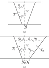 |
Figure 3. Ogilvy parametric model: (a) in the symmetric case, (b) in the non-symmetric case. |
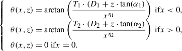
It should be noted that a rotation angle β about the out-of-plane axis can be introduced as an additional parameter to rotate all local orientations defined by θ (see, e.g., [10]). This allows for the treatment of cases where the principal axis of the weld is not aligned with the z-axis, as is commonly observed in austenitic welds.
2.3 Forward model for ToF computation
For a given ROI, the ToFs for each pair of emitter/grid node must be computed. For an isotropic medium, it is mathematically equivalent to solve the nonlinear first-order eikonal equation |∇T(x, z)| = 1/V(x, z). Here, T and V are respectively the travel time and the wave phase velocity. Several numerical approaches have been developed to solve the eikonal equation, notably Dijkstra’s algorithm, Fast Marching methods [20, 21], and ray tracing methods. In this study, a ray tracing-type algorithm is used, corresponding to the one integrated into the NDE software CIVA [22].
For a generally anisotropic, smoothly inhomogeneous material (see, e.g., [23], Sect. 3.6), the ray trajectory for a given wave mode, with slowness vector components p i and polarisation components g i as solutions of the Christoffel equation, can be determined by solving the axial ray system (also called the kinematic ray system). This system consists of two coupled ordinary differential equations (ODEs) that couple ray positions x i and ray slownesses p i with respect to the travel time T:
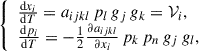
with  where c
i
j
k
l
are the components of the fourth-order stiffness tensor and ρ is the density of the material. Here, 𝒱
i
represents the components of the energy velocity vector.
where c
i
j
k
l
are the components of the fourth-order stiffness tensor and ρ is the density of the material. Here, 𝒱
i
represents the components of the energy velocity vector.
By using a multi-step iterative scheme such as Runge–Kutta and with defining initial conditions we can solve the ODEs defined by the kinematic ray system above. Noting that ray tracing algorithms do not necessitate defining an a priori spatial mesh and it allows to get simultaneously the travel time and the ray associated paths.
2.4 Principles and improvements
The core innovation of this work is to improve the approach proposed by Ménard et al. [13] by developing an algorithm that allows the automated determination of promising local ROIs in which the probability of defect presence is high, and thus optimising a global normalised imaging criterion compared to the local criterion based on the maximum amplitude. In the following, the approach for determining promising ROIs will be described, followed by the new optimisation process.
2.4.1 Local ROIs determination
In order to identify pertinent local ROIs (named subzones) within the inspected weld, the proposed approach consists of computing multiple TFM image samples using different sets of material properties generated through Sobol sampling [24] in a multidimensional bounded parameter space. Post-processing of these TFM images allows the identification of highly energetic regions, which are assumed to correspond to local defect diffracted fields. These regions are then used to define promising subzones for subsequent optimisation.
As defined previously, Ω D (0) is the global ROI enclosing the inspected weld, assumed to be known. Let 𝒳sobol denote the set of Sobol-generated samples X of the orientation and stiffness parameters. For each weld material description in 𝒳sobol, a corresponding TFM image is computed. Each TFM image is then binarised and thresholded using Otsu’s method [25].
Contours are extracted from the post-processed TFM images, and their associated bounding boxes are determined. This first step enables the identification of geometrical zones enclosing the front-wall and back-wall (bottom) echoes, as shown in Figure 4. Once these geometrical echo zones are defined, they are removed from the TFM images so that only the inspection region, excluding front and bottom echoes, is retained.
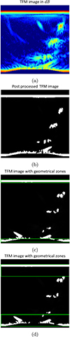 |
Figure 4. Determination of geometrical zones based on a sample of a TFM image: (a) TFM image in dB non-processed (b) TFM image processed (c) bounding boxes of front and bottom echoes (d) adapted dimensions of the bounding boxes. |
The cropped TFM images are then subjected to the same processing procedure: binarisation using Otsu thresholding, contour detection, and bounding box extraction. Let  denote the total area of white pixels in the cropped TFM image corresponding to sample k, and let
  denote the area of white pixels enclosed within a given bounding box b
b.
denote the area of white pixels enclosed within a given bounding box b
b.
In the first filtering step, all bounding boxes obtained from all samples are examined, and only those with  below a predefined threshold are retained (Fig. 5a). In the second step, we retain only the bounding boxes belonging to images for which
  is below the 10th percentile of the set
  . This two-step filtering strategy is motivated by the observation that true defect echoes tend to be more spatially focused and energetically concentrated than imaging artefacts. When incorrect material properties are used to compute TFM images, defect echoes become distorted and diffuse. Therefore, by exploring the parameter space via Sobol sampling and applying the proposed filtering criteria, the probability of isolating regions corresponding to actual defects is increased. After these two filtering steps, the remaining bounding boxes are merged to define defect subzones, as illustrated in Figure 5c. The algorithm thus outputs three types of zones: (i) zones corresponding to the front-wall echo, (ii) zones corresponding to the bottom-wall echo, and (iii) subzones associated with potential defect echoes. For example, the subzones identified and shown in Figure 6, effectively correspond to the three SDHs.
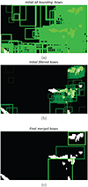 |
Figure 5. Determination of subzones including potential defects based on TFM images samples: (a) all bounded boxes having area under a certain threshold (b) kept bounded boxes of TFM images having focused energy (c) post-processed kept bounded boxes to define subzones. |
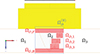 |
Figure 6. Identified subzones for a weld with three side-drilled holes. |
2.4.2 Optimisation process
The proposed optimised imaging criterion, which takes the identified subzones into account, is first presented, followed by a brief description of the newly integrated hybrid optimiser.
Optimised criterion Once the geometrical zones Ω D, F , Ω D, B , and the defect subzones Ω D, i with i ∈ 1, …, N D (where N D denotes the number of subzones) are determined (Fig. 6), a new normalised global imaging criterion is introduced. Let us define the set of indices corresponding to all relevant zones as 𝒦 D = {F, B, 1, …, N D }. For each zone index k ∈ {1, …, N D }, a reference maximum amplitude is computed as follows: for k ∈ {1, …, N D }, it is obtained by averaging the metric over all Sobol samples, while for k ∈ {F, B}, it is defined as the maximum value over all samples. This approach ensures that defect echoes have a greater influence than geometrical echoes on the optimised criterion, as the objective is to improve the quality of TFM in terms of defect detectability.
Let  denote the reference maximum amplitude associated with the grid 𝒢
D, k
. The global imaging criterion is then defined as:
denote the reference maximum amplitude associated with the grid 𝒢
D, k
. The global imaging criterion is then defined as:
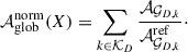
This criterion corresponds to the sum of the normalised maximum amplitudes over all zones. By construction, it introduces a notion of spatial balance, as the normalisation ensures that the echoes from all zones are weighted equally. Compared to a simple maximisation of the overall amplitude, the proposed criterion has a more physical meaning and constrains the optimisation process towards physically consistent solutions.
Similarly to the previous approach, the enhanced TFM image is obtained as I Ω D (0) (X *), where X * is obtained by solving the following optimisation problem:

Optimiser The optimised criterion behaves as a black-box objective function and exhibits multiple local minima, which motivates the use of robust global optimisation algorithms. The variant of the PSO algorithm used in [13] is a gradient-free global optimiser based on particles exploration inspired by swarm behaviour. Although this optimiser is capable of approaching the global minimum given sufficient computational resources, its performance deteriorates when the computational budget is reduced. In particular, it may suffer from reduced precision and variability between repetitions, as particles are quasi-randomly initialised using Latin Hypercube Sampling (LHS).
Based on the benchmark study reported in [15], the TikTak algorithm, detailed in Algorithm 2, has demonstrated robust performance compared to other global optimisation methods. It was therefore implemented in this work as an alternative to PSO. TikTak is a hybrid optimisation algorithm combining a global exploration phase with a subsequent local refinement phase. The global phase identifies promising regions of the search space, after which a local optimiser (BOBYQA, a gradient-free local optimisation algorithm, as used in the original work of [15], is applied) is applied to exploit the local topography of the objective function and identify multiple local minima. The global minimum is then selected as the best solution among these local minima. In addition, unlike PSO, TikTak is deterministic, as the initial sampling of points is performed using Sobol sequences, which are known for their better uniform space-filling properties compared to LHS [26]. In addition, the TikTak algorithm is well suited for parallel computing architectures, as both the global sampling phase and the subsequent local optimisation runs can be executed independently for different initial points. A parallel implementation written in Fortran 90 is available at https://github.com/serdarozkan/TikTak. However, in the present study, TikTak was implemented and executed in a sequential manner to ensure consistency with the available computational framework.
3 Application results
In this section, the results of the proposed approach are presented, along with its capability to enhance the quality of TFM images and its effectiveness in improving defect detectability. First, the approach is assessed using simulated FMC data based on the configuration shown in Figure 1. Subsequently, the method is validated using experimentally acquired FMC data to further demonstrate its practical applicability and its performance under real inspection conditions.
3.1 Results with a simulated FMC
The developed approach was first validated using simulated FMC data. The same inspection configuration presented in the previous section was used. The weld was modelled using a symmetric Ogilvy parametric representation (Fig. 7) with parameters reported in Table 1. A transversely isotropic stiffness tensor was assumed, with the z-axis defined as the axis of anisotropy (Tab. 1). The FMC data were generated using the finite element method (FEM), considering a two-dimensional formulation. Based on the simulated FMC dataset, several TFM images were reconstructed. First, a reference TFM image was obtained using the true material parameters employed in the simulation. Second, a TFM image was reconstructed under the simplifying assumption that the weld material is isotropic and homogeneous. Finally, a TFM image was produced using the proposed approach, the TikTak optimisation parameters used are reported in Table 2.
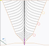 |
Figure 7. Double bevel weld with three side-drilled holes with map orientation described with Ogilvy. |
Ogilvy and stiffness parameters used in the simulated case.
Parameters used for the TikTak optimiser (defined in Algorithm 2).
The obtained results are presented in Figure 8. When assuming an isotropic and homogeneous material, the quality of the TFM image is significantly degraded compared to the reference TFM image reconstructed using the true material parameters. This degradation is primarily characterised by a substantial loss of echo amplitude. In addition, the second and third echoes are strongly distorted and can no longer be clearly identified. Thus, the degradation becomes more pronounced with increasing propagation distance within the weld, highlighting the cumulative impact of inaccurate material property assumptions on wave propagation. In contrast, the proposed approach provides a substantial improvement in image quality, both in terms of amplitude recovery and spatial accuracy. The three defect echoes are correctly reconstructed, with only minor positional deviations observed for the second and third echoes.
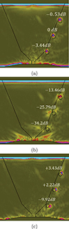 |
Figure 8. TFM images obtained with: (a) known material properties (b) with an isotropic homogeneous material (c) with the developed approach. |
One noticeable difference from the reference image is that a spatial shift of a few mm is observed at the location of the reconstructed echoes, with the shift becoming more pronounced for deeper echoes. This shift is due to the fact that the identified weld properties do not correspond exactly to the true weld properties. In fact, the true weld properties do not correspond to the properties that maximise the metric, as the metric proposed in this case is mainly focused on the first echo. However, as stated above, the goal is not to invert the weld properties but rather to improve the quality of the reconstructed TFM image. One way to improve this would be to assign a higher weight to the deepest echo, as it is more sensitive to the weld properties and may therefore constrain the metric more effectively toward the physical properties. It may also be noted that, even in the presented case, the variation from the true physical properties is negligible compared to the initial extent of the search space.
3.2 Results with an experimental FMC
As the proposed approach was validated using simulated FMC data, it was subsequently tested on experimentally acquired FMC data obtained from an OL60° inspection of a heterogeneous, anisotropic austenitic weld (see Fig. 9). The specimen contained two SDHs located at the level of the right bevel. A 64-element linear array transducer with a central frequency of 2 MHz was employed. This experimental campaign was conducted within the framework of the European project ADVISE. The numerical model of the inspected specimen is presented in Figure 9, together with the region of interest (ROI) considered for the TFM reconstruction. The weld was modelled using a symmetric Ogilvy parametric model, and the material was assumed to be transversely isotropic. For the TikTak optimisation algorithm, the same parameter settings as in the simulated case were retained. As in the simulated study, a TFM image assuming an isotropic and homogeneous material is first reconstructed. Subsequently, a TFM image obtained using the proposed approach is generated for comparison. In this experimental case, the exact material properties are unknown, therefore, no ground-truth reference image is available. Nevertheless, the geometry of the specimen and the precise locations of the SDHs are well known. Consequently, the expected echo positions can be used as a reference to assess the accuracy of the reconstructed images.
The obtained results are presented in Figure 10. Under the assumption of an isotropic and homogeneous material, the defects are not detected, and their amplitudes are of the same order of magnitude as the background noise. In contrast, when the proposed approach is applied, the echoes corresponding to the two SDHs are clearly reconstructed and accurately positioned. An amplitude gain of approximately 13 dB is observed compared to the isotropic homogeneous case. In addition, an increase in the bottom echo amplitude can be noted. These results demonstrate the capability of the proposed method to provide reliable reconstructions even when applied to experimentally acquired FMC data. It should be emphasised that the FMC data were post-processed to reduce noise prior to their use in the optimisation procedure. The FMC signals were filtered using a bandpass filter centred on the emitted signal’s central frequency.
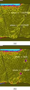 |
Figure 10. TFM images obtained: (a) with a homogeneous isotropic material (b) with the developed approach. |
4 Discussion
As demonstrated in the previous sections, the proposed approach significantly improves the quality of the TFM images in terms of both SNR and defect detectability. Promising results were obtained using both simulated and experimentally acquired FMC data. The enhanced imaging criterion introduces a global objective function, enabling a simultaneous amplification of all energetic regions in the image, including both geometrical echoes and defect-related echoes.
The TikTak optimisation algorithm provided satisfactory results while requiring significantly less computation time than PSO, as shown in the appendix (Fig. B.1). For PSO, five runs were performed using 30 particles and 20 iterations, whereas TikTak employed 150 global searches followed by 20 local searches. The five PSO runs required approximately 9 h and 14 min, while TikTak completed in approximately 2 h and 18 min. As can be seen, the TikTak solution achieved a quality comparable to that of the best PSO solution. Furthermore, in two of the PSO runs, the third SDH was poorly reconstructed. The instability observed in PSO is attributed to the use of Latin Hypercube Sampling, whereas TikTak relies on Sobol sampling. Investigating another variant of PSO that combines PSO with Sobol sampling could therefore be an interesting avenue for future work. Moreover, the proposed approach does not require any prior knowledge of the defect locations but only the global inspected ROI. In addition, the framework is not restricted to austenitic welds and can, in principle, be extended to other materials.
Nevertheless, certain limitations of the proposed approach should be highlighted. Potential defects located near the top and bottom surfaces are not explicitly considered in the current framework, as geometrical echoes are treated as large bounding boxes. To address this limitation, more advanced strategies will need to be developed to better discriminate between geometrical echoes and defect-related indications near the bottom and top surfaces. Geometrical echoes are often characterised by higher energy levels and may therefore mask weaker defect signals.
Regarding computational cost, the presented results based on experimental data required approximately 1 h of computation on an 11th Gen Intel(R) Core(TM) i9-11950H processor operating at 2.60 GHz. To make the approach more suitable for industrial applications, ongoing work focuses on reducing the dimensionality of the optimisation problem by eliminating parameters with low sensitivity to the objective function. Additionally, a more optimised computational pipeline is being developed to minimise unnecessary computational overhead. Finally, other imaging criteria beyond maximum amplitude will also be evaluated in order to identify the most robust and performant imaging metric for weld inspection.
One can further analyse the evolution of the optimised metric throughout the optimisation process using TikTak, as well as the behaviour of the local metrics within each subzone. The convergence history of the optimisation procedure is illustrated in Figure 11. The plot on the left side shows the convergence of the global normalised metric, whereas the plot on the right side presents the convergence curves of the normalised local metric evaluated in each subzone. In these plots, the solid line represents the best local search during each local search phase, while the shaded regions encompass the full range of outcomes obtained from all local searches. Two main observations can be drawn from these convergence curves. First, subzones that are weakly influenced by the weld properties exhibit relatively small variations in their local criteria, whereas zones more strongly affected, such as the SDH regions, display significantly larger variations. Second, during the local search phase, the magnitude of variation decreases with the number of iterations. This indicates that local searches initiated from the best candidates identified during the global search phase evolve with a relatively low slope, reflecting gradual refinement. In contrast, local searches starting from poorer candidates exhibit steeper slopes, indicating more pronounced improvement during early iterations. This behaviour suggests that even in scenarios where the global optimum is not reached, the best local optima identified are likely to remain close to it. Furthermore, a detailed analysis of these convergence curves can inform the selection of the number of local search phases, enabling a trade-off between computational cost and solution accuracy.
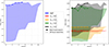 |
Figure 11. Local search phase convergence curves: (left) of the global optimised criterion (right) of each local normalised criterion computed for all subzones. |
5 Conclusion
In this work, an adaptive imaging method was proposed, building upon previous developments in model-based ultrasonic imaging. The approach aims to enhance the TFM reconstruction of an inspected weld by optimising a global normalised imaging criterion, without requiring any prior knowledge of the defect locations. The methodology consists of two main phases. The first phase involves the identification of promising subzones with a high probability of defect presence. This is achieved through a sampling strategy combined with image processing techniques. The second phase corresponds to the optimisation stage, which is performed using the previously identified subzones in order to refine the imaging model parameters. A robust hybrid optimisation algorithm, TikTak, was integrated into the framework to ensure stable and efficient convergence. The proposed approach was validated using both simulated and experimentally acquired FMC data, demonstrating promising results and enabling a partial inversion of the most influential model parameters.
Future work will focus on reducing the computational time to facilitate industrial applicability. In addition, more advanced strategies will be investigated to better manage geometrical echoes that may mask or interfere with defect-related echoes, thereby further improving the reliability and robustness of the imaging process. Finally, future work will include validation using new data, leveraging detailed knowledge of welding process parameters and the resulting microstructure. This evaluation will help assess the relevance and validity of the adaptive approach based on textured weld models.
Acknowledgments
We would like to express our sincere thanks to Edouard Demaldent for coordinating the IWeld project at the CEA, and to Jean-Baptiste Blanc-Rouchosse for his expertise regarding the CIVASERVER framework, which was used in this work.
Funding
This study was partly funded by the European IWeld project, which received funding from the EURATOM research and training programme 2021–2027 under grant agreement number 101061359 https://cordis.europa.eu/project/id/101061359/fr.
Conflicts of interest
The authors declare that they have no known competing financial interests or personal relationships that could have appeared to influence the work reported in this paper.
Data availability statement
Data are available on request from the authors.
Author contribution statement
Ali Boukham: Conceptualisation, Methodology, Formal analysis, Software, Writing – original draft. Jordan Barras: Conceptualisation, Methodology, Software, Writing – Review & Editing. Maxance Marmonier: Software, Writing – Review & Editing. Nicolas Leymarie: Conceptualisation, Supervision, Writing – Review & Editing.
References
- L. Le Jeune, S. Robert, P. Dumas, A. Membre, C. Prada: Adaptive ultrasonic imaging with the total focusing method for inspection of complex components immersed in water, in: AIP Conference Proceedings. Vol. 1650. American Institute of Physics, 2015, pp. 1037–1046. https://doi.org/10.1063/1.4914712. [Google Scholar]
- J. Camacho, C. Fritsch: Adaptive Beamforming by Phase Coherence Processing. INTECH Open Access Publisher, 2011. [Google Scholar]
- J. Camacho, M. Parrilla, C. Fritsch: Phase coherence imaging. IEEE Transactions on Ultrasonics, Ferroelectrics, and Frequency Control 56, 5 (2009) 958–974. [Google Scholar]
- R. Baiotto, B. Knight-Gregson, C. Nageswaran, T. Clarke: Coherence weighting applied to FMC/TFM data from austenitic CRA clad lined pipes. Journal of Nondestructive Evaluation 37, 3 (2018) 49. [Google Scholar]
- J. Cruza, J. Camacho, C. Fritsch: Plane-wave phase-coherence imaging for NDE. NDT & E International 87 (2017) 31–37. [Google Scholar]
- J.R. Tempelman, A.J. Wachtor, E.B. Flynn: Machine learning-based ultrasonic weld characterization using hierarchical wave modeling and diffusion-driven distribution alignment, 2025. ArXiv preprint arXiv:https://arxiv.org/abs/2510.13023. https://doi.org/10.1016/j.cma.2026.118899. [Google Scholar]
- J. Singh, K. Tant, A. Mulholland, C. MacLeod: Deep learning based inversion of locally anisotropic weld properties from ultrasonic array data. Applied Sciences 12, 2 (2022) 532. [Google Scholar]
- H. Zhou, Z. Han, D. Du: An improved ultrasonic imaging method for austenitic welds based on grain orientation distribution inversion algorithm. Journal of Nondestructive Evaluation 39, 3 (2020) 54. [Google Scholar]
- Q. Liu, H. Wirdelius: Estimation of grain orientation in an anisotropic weld by using a model of ultrasonic propagation in an inverse scheme. Modelling and Simulation in Engineering 2014, 1 (2014) 637476. [Google Scholar]
- M.K. Kalkowski, M.J. Lowe, V. Samaitis, F. Schreyer, S. Robert: Weld map tomography for determining local grain orientations from ultrasound. Proceedings of the Royal Society A: Mathematical, Physical and Engineering Sciences 479, 2277 (2023) 20230236. [Google Scholar]
- J. Ludlam, K.M. Tant, A. Curtis, V. Dolean: Ultrasonic travel-time tomography for approximating the local elastic tensor in complex media, in: 2025 IEEE International Ultrasonics Symposium (IUS). IEEE, 2025, pp. 1–5. https://doi.org/10.1109/IUS62464.2025.11201431. [Google Scholar]
- K.M. Tant, E. Galetti, A. Mulholland, A. Curtis, A. Gachagan: Effective grain orientation mapping of complex and locally anisotropic media for improved imaging in ultrasonic non-destructive testing. Inverse Problems in Science and Engineering 28, 12 (2020) 1694–1718. [Google Scholar]
- C. Ménard, S. Robert, R. Miorelli, D. Lesselier: Optimization algorithms for ultrasonic array imaging in homogeneous anisotropic steel components with unknown properties. NDT & E International 116 (2020) 102327. [Google Scholar]
- C. Menard, S. Robert, D. Lesselier: Ultrasonic array imaging of nuclear austenitic V-shape welds with inhomogeneous and unknown anisotropic properties. Applied Sciences 11, 14 (2021) 6505. [Google Scholar]
- A. Arnoud, F. Guvenen, T. Kleineberg: Benchmarking global optimizers. Technical Report, National Bureau of Economic Research, 2019. https://doi.org/10.3386/w26340. [Google Scholar]
- I.C. Trelea: The particle swarm optimization algorithm: convergence analysis and parameter selection. Information Processing Letters 85, 6 (2003) 317–325. [Google Scholar]
- S. Mahaut, M. Darmon, S. Chatillon, F. Jenson, P. Calmon: Recent advances and current trends of ultrasonic modelling in CIVA. Insight-Non-Destructive Testing and Condition Monitoring 51, 2 (2009) 78–81. [Google Scholar]
- M. Darmon, N. Leymarie, S. Chatillon, S. Mahaut: Modelling of scattering of ultrasounds by flaws for NDT, in: A. Leger, M. Deschamps, Eds. Ultrasonic Wave Propagation in non Homogeneous Media. Springer, Berlin, Heidelberg, 2009, pp. 61–71. [Google Scholar]
- J. Ogilvy: Computerized ultrasonic ray tracing in austenitic steel. NDT International 18, 2 (1985) 67–77. [Google Scholar]
- K.M.M. Tant, E. Galetti, A.J. Mulholland, A. Curtis, A. Gachagan: Effective grain orientation mapping of complex and locally anisotropic media for improved imaging in ultrasonic non-destructive testing. Inverse Problems in Science and Engineering 28, 12 (2020) 1694–1718. [Google Scholar]
- J.A. Sethian: Fast marching methods. SIAM Review 41, 2 (1999) 199–235. [Google Scholar]
- N. Leymarie, A. Imperiale, T. Fortuna, E. Demaldent: Comparisons of ray and finite element simulations of ultrasonic wave fields in smoothly inhomogeneous austenitic welds of thick-walled components. NDT & E International 147 (2024) 103177. [Google Scholar]
- V. Cerveny: Seismic Ray Theory. Cambridge University Press, 2005. [Google Scholar]
- I.M. Sobol’, D. Asotsky, A. Kreinin, S. Kucherenko: Construction and comparison of high-dimensional Sobol’generators. Wilmott 2011, 56 (2011) 64–79. [Google Scholar]
- P.-S. Liao, T.-S. Chen, P.-C. Chung, et al.: A fast algorithm for multilevel thresholding. Journal of Information Science and Engineering 17, 5 (2001) 713–727. [Google Scholar]
- M. Renardy, L.R. Joslyn, J.A. Millar, D.E. Kirschner: To Sobol or not to Sobol? The effects of sampling schemes in systems biology applications. Mathematical Biosciences 337 (2021) 108593. [Google Scholar]
Appendix A
Optimisation algorithms
Require: Objective function f: ℝn → ℝ
Bounds Xmin, Xmax ∈ ℝn
Number of particles Np
Maximum iterations Nmax
Hot-reload trigger iteration Nhr
Maximum hot-reload usage Nhrmax
Coefficient of variation threshold cv ∈ ℝn
Ensure: Approximate solution X* ≈ arg minX f(X)
## Initialisation: iteration index
1: k ← 1
## Initialisation: hot-reload counter
2: h ← 0
## Generate initial particle positions using Latin Hypercube Sampling (LHS)
3: ![Mathematical equation: $ \{X_i^0\}_{i=1}^{N_p} \leftarrow \text{LHS}\left(N_p, [X^{\min}, X^{\max}]\right) $](/articles/aacus/full_html/2026/01/aacus260094/aacus260094-eq19.gif)
## Generate initial particle velocities randomly within bounds
4: ![Mathematical equation: $ \{v_i^0\}_{i=1}^{N_p} \leftarrow \text{Rand}\left(N_p, [X^{\min}, X^{\max}]\right) $](/articles/aacus/full_html/2026/01/aacus260094/aacus260094-eq20.gif)
## Initialise particle best positions with initial positions
5: 
## Initialise global best as the best among personal bests
6: 
7: while k ≤ Nmax do
8: if k = Nhr then
## Hot-reload triggered: reinitialise particle positions using LHS and increment hot-reload counter
9: ![Mathematical equation: $ \{X_i^k\}_{i=1}^{N_p} \leftarrow \text{LHS}\left(N_p, [X^{\min}, X^{\max}]\right) $](/articles/aacus/full_html/2026/01/aacus260094/aacus260094-eq23.gif)
10: h ← h + 1
11: end if
12: for i = 1, …, Np do
## Update particle positions based on velocity, personal best, and global best
13: 
## Update particle best if current position is better
14: 
15: end for
## Update global best based on current personal bests
16: 
## Stop if convergence criterion based on coefficient of variation is met
17: if  ≤ Cv then
18: break
19: end if
## Stop if maximum hot-reload usage reached
20: if  then
then
21: break
22: end if
23: k ← k + 1
24: end while
## Return the best solution found
25: X* ← gk
Require: Objective function f(X), X ∈ ℝn;
Bounds [Xjmin, Xjmax], j = 1, …, n;
Global points Ng;
local searches Nl;
Shrink threshold Ns;
local optimiser Oploc;
Max local iterations Niter;
position tolerance ϵx;
value tolerance ϵy
Ensure: Approximate solution X* ≈ arg minX f(X)
## Global Search phase
## Generate Sobol points
1: ![Mathematical equation: $ \{X^{(i)}\}_{i=1}^{N_g} \leftarrow \text{Sobol}\left(N_g, \prod_j [X_j^{\min}, X_j^{\max}]\right) $](/articles/aacus/full_html/2026/01/aacus260094/aacus260094-eq29.gif)
## Evaluate f(i) = f(X(i)) sort ascending
2: {X(i)} ← sorted({X(i)}, f(i))
## End of Global Search phase
## Local Search phase
## Initialise
3: f* ← ∞, X* ← none
4: for i = 1 to Nl do
## Pick i-th best candidate X(i)
5: if i > Ns then
## Shrink towards current best
6: 
7: end if
## Run local optimizer
8: (Xloc, floc) = Oploc(X(i), Niter, ϵx, ϵy)
## Update the best solution found
9: if floc < f* then
10: f* ← floc, X* ← Xloc
11: end if
12: end for
Appendix B
Comparison of PSO and TikTak results
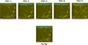 |
Figure B.1. Comparison of the results obtained using PSO and TikTak in the simulated case. Five independent runs were performed with PSO, using 30 particles and 20 iterations per run, while TikTak was configured with 150 global search points and 20 local searches. |
Cite this article as: Boukham A. Barras J. Marmonier M. & Leymarie N. 2026. Improving defect detection of nuclear welds using adaptive imaging based on uncertain material parameters optimization. Acta Acustica, 10, 71. https://doi.org/10.1051/aacus/2026069.
All Tables
All Figures
|
Figure 1. Configuration of the simulated FMC. |
| In the text | |
|
Figure 2. Schematic representation of the three domains Ω1, Ω2, and Ω3, corresponding to the base metal and the weld, together with the global region of interest Ω D (0) and the local region of interest Ω D . |
| In the text | |
|
Figure 3. Ogilvy parametric model: (a) in the symmetric case, (b) in the non-symmetric case. |
| In the text | |
|
Figure 4. Determination of geometrical zones based on a sample of a TFM image: (a) TFM image in dB non-processed (b) TFM image processed (c) bounding boxes of front and bottom echoes (d) adapted dimensions of the bounding boxes. |
| In the text | |
|
Figure 5. Determination of subzones including potential defects based on TFM images samples: (a) all bounded boxes having area under a certain threshold (b) kept bounded boxes of TFM images having focused energy (c) post-processed kept bounded boxes to define subzones. |
| In the text | |
|
Figure 6. Identified subzones for a weld with three side-drilled holes. |
| In the text | |
|
Figure 7. Double bevel weld with three side-drilled holes with map orientation described with Ogilvy. |
| In the text | |
|
Figure 8. TFM images obtained with: (a) known material properties (b) with an isotropic homogeneous material (c) with the developed approach. |
| In the text | |
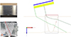 |
Figure 9. Inspection configuration of the experimentally acquired FMC [14]. |
| In the text | |
|
Figure 10. TFM images obtained: (a) with a homogeneous isotropic material (b) with the developed approach. |
| In the text | |
|
Figure 11. Local search phase convergence curves: (left) of the global optimised criterion (right) of each local normalised criterion computed for all subzones. |
| In the text | |
|
Figure B.1. Comparison of the results obtained using PSO and TikTak in the simulated case. Five independent runs were performed with PSO, using 30 particles and 20 iterations per run, while TikTak was configured with 150 global search points and 20 local searches. |
| In the text | |
Current usage metrics show cumulative count of Article Views (full-text article views including HTML views, PDF and ePub downloads, according to the available data) and Abstracts Views on Vision4Press platform.
Data correspond to usage on the plateform after 2015. The current usage metrics is available 48-96 hours after online publication and is updated daily on week days.
Initial download of the metrics may take a while.