


| Issue |
Acta Acust.
Volume 10, 2026
Topical Issue - Proceedings of AFPAC 2026
|
|
|---|---|---|
| Article Number | 66 | |
| Number of page(s) | 12 | |
| DOI | https://doi.org/10.1051/aacus/2026062 | |
| Published online | 27 July 2026 | |
Scientific Article
Self-adaptive transcranial ultrasound imaging using an effective skull model: experimental evaluation on a human skull at 3.15 MHz
1
Université Paris-Saclay, CEA, List, Gif-sur-Yvette, France
2
Université Paris-Saclay, CNRS, Inserm, CEA, BioMaps UMR 9011, Gif-sur-Yvette, France
3
Sorbonne Université, LIB Inserm U 1146, CNRS UMR 7371, Paris, France
* Corresponding author: This email address is being protected from spambots. You need JavaScript enabled to view it.
Received:
30
March
2026
Accepted:
19
June
2026
Abstract
Introduction. Transcranial ultrasound imaging is hindered by skull-induced aberrations that degrade focusing and image contrast. Existing correction methods typically rely on external imaging or detailed acoustic models, limiting their applicability in emergency settings. Methods. We propose an adaptive approach based on an effective skull model comprising two interfaces and an effective velocity, estimated directly from Full Matrix Capture data without external information. The estimated parameters are integrated into a Total Focusing Method reconstruction with refraction correction. The method is evaluated experimentally at 3.15 MHz by imaging wire targets located beyond a human skull fragment in four configurations: free-field reference, uncorrected, skull corrected with automatically estimated parameters, and skull corrected with optically scanned surfaces. Results. The effective model reduces the mean Euclidean localization error by 67% (2.16 to 0.71 mm). Comparison with the optical reference isolates interface estimation uncertainty as the dominant residual error source, while confirming that the effective velocity model itself produces comparable performance when provided with accurate interface positions. Discussion. These results demonstrate that a self-estimated model enables reliable localization in transcranial conditions. Improving surface estimation robustness is identified as a key factor for precise target reconstruction.
Key words: Transcranial ultrasound imaging / Effective skull model / Adaptive aberration correction / Full Matrix Capture / Total Focusing Method
© The Author(s), Published by EDP Sciences, 2026
 This is an Open Access article distributed under the terms of the Creative Commons Attribution License (https://creativecommons.org/licenses/by/4.0), which permits unrestricted use, distribution, and reproduction in any medium, provided the original work is properly cited.
1 Introduction
1.1 Context
Brain imaging currently relies primarily on computed tomography (CT) and magnetic resonance imaging (MRI). Both modalities provide reliable diagnoses, but they are difficult to access in pre-hospital emergency settings or at the bedside in intensive care units. Ultrasound offers advantages for these situations: it is portable, inexpensive, and immediately available [1].
However, transcranial ultrasound imaging remains particularly challenging due to the presence of the skull, whose high acoustic impedance significantly impairs the propagation of the ultrasonic waves. Furthermore, the skull exhibits a complex, multilayered structure, composed of two cortical bone layers enclosing the diploë, with pronounced spatial variations in thickness, density, and velocity. This heterogeneity results in substantial attenuation, beam distortion due to refraction at the interfaces, and phase aberrations arising from spatial variations in skull thickness and velocity, leading to defocusing. This results in severe degradation of ultrasound images in terms of resolution, contrast, and signal-to-noise ratio [2, 3].
1.2 State of the art
Several families of methods have been proposed to correct these aberrations.
Time reversal and inverse filter techniques allow the determination of optimal delay and amplitude laws to compensate for wavefront distortion through the skull [4]. These methods are effective, but they require control points placed in the imaging region. They are therefore invasive and not applicable in clinical imaging.
A second family of approaches relies on a propagation model through the skull, built from a morphological description obtained by CT [4] or MRI. These approaches allow non-invasive computation of corrections. However, they require prior acquisition of external imaging and modeling of the acoustic properties of the medium [2, 5]. This increases data and computational requirements and limits their use in emergency contexts [2, 3].
A third family of approaches estimates propagation parameters directly from ultrasound data, without resorting to external imaging [6]. Hajian et al. [7] demonstrated 3D skull profile extraction combined with adaptive sound speed estimation using a custom matrix array in pulse-echo, achieving thickness measurement accuracies of 4.2% on cranial bone phantoms. More recently, Waasdorp et al. [8] proposed an adaptive 4-layer ray-tracing beamformer for transcranial Doppler imaging in rats, with iterative estimation of the sound speed in each layer, yielding a 32% gain in lateral resolution compared with constant-velocity delay-and-sum. These approaches reduce the requirements for prior information, but the question of the trade-off between model simplicity, robustness of parameter estimation, and reconstruction quality remains open.
A complementary family of approaches relies on in vivo guide-star signals to estimate aberration profiles. Robin et al. [9] used contrast microbubbles as natural guide stars to estimate, within isoplanatic patches, both the aberration phase profile and an effective sound speed, applied directly in beamforming. This strategy provided a mean Doppler contrast gain of 4 dB and a 38% increase in detected microbubble tracks in clinical transcranial ultrasound localization microscopy. Such methods, however, require contrast agent injection and are therefore not applicable to native imaging in emergency contexts.
1.3 Problem statement
In this work, the imaging process is based on Full Matrix Capture acquisition and data processing using the Total Focusing Method (TFM) algorithm [10]. This imaging process relies on the estimation of ultrasonic times-of-flight (ToF) between each probe element and each point in the imaging region. To simplify this process for real-time computation, a simplified model of the cranial wall as a homogeneous and isotropic medium has been proposed. The adaptive approach thus consists, from FMC ultrasound data and without resorting to any other imaging modality, in estimating the parameters of this structure, namely (i) the geometry of the two interfaces between the skull and soft tissues and (ii) the longitudinal wave velocity in the equivalent homogeneous medium modelling skull bone tissue.
2 Physical framework and imaging formulation
2.1 Full Matrix Capture acquisition
Data are acquired using an FMC scheme [10] with a phased array probe of N elements. For each sequence, a single element is active in transmission while all elements receive simultaneously. The operation is repeated for each of the N elements, producing N × N temporal signals S ij (t) that contain the complete information on the acoustic interactions in the medium. The experiments are analyzed in a two-dimensional framework; element positions are denoted x i , and a point in the imaging domain is denoted r = (x, z), where z is the imaging depth.
2.2 TFM reconstruction
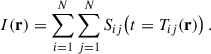
The principle of the TFM algorithm [10] is the coherent summation of signals from an FMC acquisition, ensuring focusing in both transmission and reception at each point of the imaging region. The reconstruction involves two steps. The first step consists in computing the ToF T ij (r) between each transmitter–receiver pair (i, j) and each point r. For each image point, N × N ToF must be computed. The acoustic path between an element and a point r crosses three media: water, the cranial wall, and the intracranial medium. At each interface, the ultrasound ray path is refracted according to Snell’s law [2]. The total ToF is the sum of the forward path (transmission from element i to point r) and the return path (from point r to receiving element j): Tij (r)=T i (r)+T j (r). This computation requires knowledge of the skull interface geometry and the propagation velocity in bone. The accuracy of these ToF directly determines the focusing quality. Figure 1 illustrates the refracted paths for two elements i and j toward a point r.
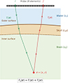 |
Figure 1. Refracted paths through the skull. Green: forward path from transmitting element i to point r. Red: return path from point r to receiving element j. |
 (1)
(1)
The second step consists in coherently summing the N × N signals, each delayed by the corresponding ToF, as expressed by the formula above. The signals are temporally interpolated and an analytical envelope is computed using the Hilbert transform.
3 Parameter estimation method
As stated in Section 2.2, ToF computation requires knowledge of the skull interfaces and the propagation velocity in bone. The proposed method consists in estimating them directly from the acquired FMC data. The procedure is organized in five steps: (1) initial TFM reconstruction in a homogeneous medium, (2) outer surface detection, (3) estimation of the effective longitudinal speed of sound in skull bone tissue c eff by autofocus, (4) detection and refinement of the inner surface, (5) final reconstruction integrating the estimated parameters into a TFM reconstruction that explicitly accounts for the interfaces and refraction.
3.1 Outer surface detection
On the homogeneous TFM image, the reflection at the first interface generates a dominant amplitude discontinuity, related to the large impedance contrast between water and bone. This dominance motivates a column-wise first-crossing strategy, where the outer surface is identified as the shallowest depth at which the reflected amplitude becomes locally significant.
The detection is performed on the TFM image expressed in decibels and proceeds as follows. The image is first restricted to a realistic depth window bracketing the expected outer surface position. For each column x, a column-wise threshold is defined as
 (2)
(2)
where Δrel = −9 dB is a relative offset below the column maximum. The detected outer surface depth z out(x) is then the smallest depth in the window where the amplitude exceeds this threshold:
 (3)
(3)
The threshold is therefore local (one value per column) and relative (referenced to the column maximum), which makes the detection robust to lateral variations in attenuation and to the absolute amplitude calibration of the image.
Columns for which no sample exceeds τ(x) are filled by piecewise cubic Hermite interpolation (PCHIP) from neighboring valid columns. The resulting profile is then smoothed along the lateral direction by a Gaussian filter (standard deviation σ = 1 mm), enforcing the lateral continuity expected from the underlying anatomical surface. A cubic spline is finally fitted to the smoothed profile to provide a continuous representation z out(x) and its derivative dz out/dx, both required for refraction computation through Snell’s law in the subsequent reconstruction steps. Figure 2 illustrates the result.
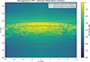 |
Figure 2. Detected outer surface (blue line) on the homogeneous TFM image. The dashed red rectangle indicates the region of interest used for the Brenner autofocus criterion. |
3.2 Estimation of ceff by autofocus
Once the outer surface is known, the longitudinal speed of sound c eff in the equivalent homogeneous medium representing bone tissue is estimated by an autofocus procedure. The principle is to reconstruct the TFM image for a set of candidate velocities and to retain the value that maximizes a sharpness criterion evaluated on a region of interest located beyond the outer surface, where the bone-induced aberrations are expected to manifest.
The sharpness is quantified by the Brenner criterion [11, 12], which measures the energy of spatial intensity gradients and favors reconstructions with sharp transitions:
 (4)
(4)
where I c (x, z) denotes the TFM image reconstructed with candidate velocity c, (x, z) are pixel coordinates within the region of interest (ROI), and the sum runs over all pixels of the ROI. The two-pixel step reduces sensitivity to high-frequency noise while preserving the response to sharp anatomical transitions.
A region of interest is defined between 1 mm and 6 mm below the detected outer surface. The lower bound is set to exclude the outer interface reflection itself, whose dominant amplitude would otherwise saturate the Brenner criterion without reflecting the quality of propagation within the bone. The upper bound is chosen to remain within the cranial wall, given its typical thickness in the studied fragment (6–8 mm), so that the sharpness criterion captures the effect of c eff on propagation through bone tissue without including the inner surface or the medium beyond. For each candidate velocity c ∈ [2000, 3000] m/s, consistent with values reported in the literature [13, 14], a TFM reconstruction is performed with refraction at the outer surface. The images are normalized in amplitude and the Brenner criterion is computed. The effective velocity is estimated as the one maximizing the Brenner criterion: c eff = argmax c B(c). Figure 3 shows a well-defined maximum at ceff = 2340 m/s.
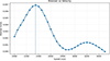 |
Figure 3. Brenner criterion as a function of candidate velocity. Maximum at c eff = 2340 m/s. |
3.3 Inner surface detection
From the reconstruction corresponding to c eff, a first estimate of the inner surface is obtained by looking for amplitude maxima at a depth compatible with skull thickness. Unlike the outer surface, the reflection at this interface is weaker, requiring spatially constrained analysis.
A refinement is then performed by dynamic programming [15] within a ±1 mm corridor, minimizing a cost function combining a data term (high amplitudes) and a regularization term (profile continuity), whose relative weights are set empirically. This procedure produces a smooth and physically realistic profile.
4 Experimental protocol
4.1 Setup and instrumentation
Experiments are carried out in a water tank with a P4-2gH probe (96 elements, 0.2 mm pitch, 3.15 MHz center frequency) [16] mounted on a UR5 robotic arm (Universal Robots). Signals are acquired using a Verasonics Vantage 256-channel system. The setup is shown in Figure 4.
 |
Figure 4. Experimental setup. Left: schematic diagram. Right: photograph of the setup. |
For these experiments, a fragment of human skull is degassed (6–8 mm thick) and positioned in a holder. The targets are placed beyond the skull and consist of eight metallic wires (labeled F1 to F8) with a diameter of 500 μm, arranged in two rows separated by 3 mm, with a lateral spacing of 3 mm between wires within each row. Two FMC acquisitions are performed:
-
FMCwater: acquisition on the wires placed in water (reference configuration).
-
FMCskull: acquisition with the skull sample interposed between the probe and the wires.
The skull is inserted without modifying the wire positions relative to the probe, allowing direct comparison of the effects of propagation through the cranial wall and evaluation of the different corrections applied a posteriori. Acquisition parameters are kept constant for all experiments.
4.2 Wire imaging protocol
The TFM algorithm is applied to these two FMC acquisitions to obtain an image of the metallic wires in the following four configurations:
-
The FMCwater acquisition is used to obtain a reference image of the wires immersed in water, without skull (WIRES).
-
The FMCskull data are reconstructed without aberration correction: the skull is ignored and the propagation medium is assumed homogeneous (water only) (HOM).
-
The FMCskull data are reconstructed with aberration correction based on the outer and inner surfaces and the propagation velocity estimated in the adaptive process (FINAL).
-
The FMCskull data are reconstructed with aberration correction based on surfaces extracted from the STL model and the parameter c eff = 2340 m/s estimated by autofocus (STL).
4.3 Interface validation
The automatically estimated surfaces are compared to 2D cross-sections extracted from STL models of the skull obtained by optical scanning (Fig. 5).
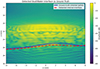 |
Figure 5. Detected inner surface (red dashes) vs. 2D cross-section of the STL model registered to the outer surface (solid blue). |
The STL model thus serves a dual role in this work: it provides a geometric reference for visual validation of the estimated surfaces, and a basis for the STL reconstruction configuration described in Section 4.2. In both cases, it constitutes a better approximation of the actual geometry than the automatic estimation, without being an exact representation.
4.4 Evaluation metrics
Four complementary metrics are used:
-
Localization accuracy is evaluated by the lateral (Δx), axial (Δz), and Euclidean distance (Δd) errors between the energy-weighted centroids (−6 dB threshold) and the reference positions.
-
Field similarity is measured by the normalized cross-correlation coefficient (NCC) computed between the reference patch (WIRES) and the patch obtained in the evaluated configuration. The patches are extracted from the energy images Eref(x, z)=|Iref(x, z)|2 and Etest(x, z)=|Itest(x, z)|2, centered on the energy-weighted barycenter of each wire. To focus the comparison on the main lobe, the NCC is evaluated on a mask M defined on the reference patch as the set of pixels whose energy lies in the top 10% of the patch values. The same mask is then applied at identical relative positions to the evaluated patch: See equation (5) at the bottom on the page.
![Mathematical equation: $$ \begin{aligned}&\mathrm{NCC} \nonumber \\&= \frac{\displaystyle \sum _{(x,z) \in M} \left[ E_{\mathrm{test} }(x,z) - \overline{E_{\mathrm{test} }} \right] \left[ E_{\mathrm{ref} }(x,z) - \overline{E_{\mathrm{ref} }} \right]}{\displaystyle \sqrt{\sum _{(x,z) \in M} \left[ E_{\mathrm{test} }(x,z) - \overline{E_{\mathrm{test} }} \right]^{2} \, \sum _{(x,z) \in M} \left[ E_{\mathrm{ref} }(x,z) - \overline{E_{\mathrm{ref} }} \right]^{2}}} \end{aligned} $$](/articles/aacus/full_html/2026/01/aacus260098/aacus260098-eq5.gif) (5)
(5)where
 and
and  denote the means of E
ref and E
test computed over the mask M. A value close to 1 indicates that the focal-spot energy distribution in the evaluated configuration matches that of the unaberrated reference; lower values indicate distortion of the lobe shape.
denote the means of E
ref and E
test computed over the mask M. A value close to 1 indicates that the focal-spot energy distribution in the evaluated configuration matches that of the unaberrated reference; lower values indicate distortion of the lobe shape. -
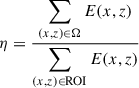
The energy concentration η quantifies how much of the local image energy is concentrated within a focal-spot-shaped region. The shape of this region is defined once on the WIRES reference image and reused on the configuration under evaluation. Specifically, for each wire, a binary mask Ωref is built on the WIRES image as the connected set of pixels whose amplitude lies within −6 dB of the local maximum. This mask captures the geometry of the reference focal spot. To evaluate a configuration, the same mask is then translated so that its center coincides with the energy-weighted barycenter of the local maximum in that configuration, yielding a repositioned mask Ω of identical shape. The energy concentration is computed on the corresponding patch as
 (6)
(6)
where E(x, z)=|I(x, z)|2 is the pixel-wise energy of the TFM image, ROI is the local sub-image enclosing the wire, Ω ⊂ ROI is the repositioned reference mask, and the sums run over all pixels of each set. A value of η close to the WIRES reference indicates that the focal spot in the evaluated configuration occupies the same energetic footprint as the unaberrated reference, while a lower value indicates an energetically more diffuse reconstruction.
-
The contrast-to-noise ratio (CNR) quantifies the visibility of each wire relative to the background:
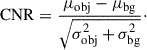 (7)
(7)
5 Results
Performance is evaluated on 8 metallic wires imaged through a human skull fragment. The TFM images obtained in the four configurations are presented in Figure 6.
 |
Figure 6. TFM images of 8 metallic wires through a human skull fragment. From left to right: WIRES (free-field reference in water), HOM (uncorrected, homogeneous medium assumption), FINAL (correction with self-estimated parameters), STL (correction with optically scanned surfaces). |
5.1 Localization accuracy
Mean localization errors are reported in Table 1.
Mean localization errors (8 wires) for the three configurations: HOM (uncorrected), FINAL (self-estimated correction), and STL (optical surface correction). Gain is relative to HOM.
Both corrected configurations substantially reduce the mean Euclidean error compared to HOM. The dominant reduction is on the axial error, consistent with the correction of the mean bias on ToF in bone, which projects predominantly along the depth direction.
STL produces a lower mean Euclidean error than FINAL (0.55 mm vs. 0.71 mm) and a reduced dispersion (σ = 0.20 mm vs. 0.49 mm). This difference is driven by two wires, F1 and F5 (see Fig. 7), for which FINAL produces localization errors of 1.76 mm and 1.10 mm respectively, while STL reduces them to 0.43 mm and 0.71 mm. For the six other wires, FINAL and STL produce comparable performance, with a mean Euclidean distance of 0.47 mm for FINAL vs. 0.45 mm for STL.
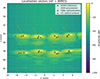 |
Figure 7. Localization vectors. Segments represent the distance between the wire localization with each method and their actual position. Blue circles: WIRES. Orange crosses: HOM. Green squares: FINAL. Red triangles: STL. |
The residual error of FINAL is therefore localized and not systematic. It affects two specific positions, F1 and F5, for which the automatic estimation of the outer and inner surfaces introduces a local inaccuracy sufficient to significantly degrade localization. STL, which constitutes a better approximation of the actual geometry, partially corrects these cases.
Figure 7 illustrates these behaviors. F1 and F5 are identifiable as the only cases where FINAL deviates significantly from the reference while STL remains close.
5.2 Focal lobe structure and local metrics
Local reconstruction quality is analyzed using the NCC and the energy ratio η defined in Section 4.4. Mean values are reported in Table 2 and per-wire results are shown in Figures 8 and 9.
Mean local metrics (8 wires).
 |
Figure 8. NCC per wire. Orange: HOM. Green: FINAL. Red: STL. |
 |
Figure 9. Energy ratio η per wire. Orange: HOM. Green: FINAL. Red: STL. |
HOM produces a compact but systematically displaced lobe: its NCC and η values reflect the local coherence of a concentrated spot around a mispositioned maximum, not the absolute reconstruction quality. After correction, the maximum is recentered toward the actual reflector position, but the lobe structure depends on the accuracy of the surfaces used.
FINAL degrades NCC and η compared to HOM: NCC drops from 0.544 to 0.458 and η from 0.333 to 0.287. STL, on the other hand, restores NCC above HOM (0.576) and improves η beyond HOM (0.363). The comparison between FINAL and STL is a controlled one: both configurations rely on the same effective model, the same value of c eff = 2340 m/s estimated by autofocus, and the same FMC data. The only quantity that differs between the two is the description of the outer and inner interfaces, automatically estimated from the data in FINAL and extracted from the optical scan in STL. Since STL reproduces or exceeds the HOM values for both NCC and η, the effective model itself cannot be the cause of the FINAL degradation: an identical model, fed with more accurate surfaces, recovers and improves the local lobe quality. The drop observed in FINAL is therefore attributable to the residual inaccuracy of the automatically estimated surfaces, which manifests both locally on the focal position (most visibly for F1 and F5) and diffusely on the energy structure of the lobe across all wires.
5.3 Contrast-to-noise ratio
The mean CNR increases from 2.39 ± 0.19 in HOM to 2.48 ± 0.18 in FINAL and 2.44 ± 0.16 in STL (Fig. 10). These moderate and comparable changes between FINAL and STL indicate that the local visibility of reflectors relative to the background is preserved in both corrected configurations. The contrast remains limited by bone attenuation and measurement noise, phenomena not accounted for in the effective model, which dominate the amplitude dynamics regardless of the correction.
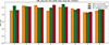 |
Figure 10. CNR per wire. Orange: HOM. Green: FINAL. Red: STL. |
5.4 Summary of results
FINAL reduces the mean Euclidean error by 67% (2.16 → 0.71 mm) and preserves CNR (2.39 → 2.48), but degrades NCC (0.544 → 0.458) and η (0.333 → 0.287). STL reduces the error by 74% (2.16 → 0.55 mm) with lower dispersion, and simultaneously improves NCC (0.576), η (0.363), and CNR (2.44). The interpretation of these differences is developed in Section 6.
6 Discussion
6.1 Physical nature of the correction and model limitations
The effective model relies on representing the cranial wall as a homogeneous and isotropic medium, described by the outer and inner interfaces and the ultrasonic wave velocity of the equivalent homogeneous medium c eff = 2340 m/s, estimated by autofocus (Fig. 3). We have proposed a methodology enabling robust estimation of these parameters from FMC data alone, without resorting to external imaging, prior calibration, or prior information on the internal skull structure.
Using this simplified description in the TFM image formation process leads to a reduction of the mean Euclidean error from 2.16 mm to 0.71 mm. This result confirms that the dominant error in HOM configuration is related to a systematic bias on ToF, correctable at first order. This bias projects predominantly along the axial direction, which explains the dominance of the gain on Δz (84%).
The STL configuration allows partial decomposition of the residual error sources of FINAL. It should be noted that STL is not an absolute ground truth: it is derived from an optical scanner on cranial bone, with its own measurement and registration inaccuracies. It constitutes a better approximation of the actual surfaces, without reproducing them exactly.
Regarding localization, STL and FINAL produce comparable mean gains (74% vs. 67%). For the majority of wires, both configurations produce equivalent performance. For F1 and F5, the automatic estimation of the outer and inner surfaces introduces a local inaccuracy that degrades FINAL localization, partially corrected by STL. These two positions constitute the limiting cases of the estimation pipeline in the experimental configuration studied, and their identification provides useful information for guiding future developments.
Regarding focal spot metrics, STL improves NCC and η compared to HOM, with CNR remaining comparable. This result establishes that the degradation of NCC and η observed in FINAL is not inherent to the effective model correction itself: STL, which uses the same c eff, demonstrates that a better surface approximation suffices to improve these metrics. The degradation is attributable to the uncertainty on the automatically estimated surfaces, which manifests at two levels: locally on the focal position for F1 and F5, and diffusely on the energy structure of the lobe for all wires.
The intrinsic limitations of the scalar effective model nonetheless remain, independent of surface quality: uniform velocity in bone, near-normal paths, two-dimensional geometry. These simplifications do not allow compensation for spatial velocity variations, bone anisotropy, or fine interface irregularities. Furthermore, even with perfectly known surfaces and exact velocity at every point, transcranial TFM reconstruction would not converge toward WIRES: bone attenuation, multiple scattering, and three-dimensional effects constitute irreversible information losses within this framework.
A further consideration concerns the type of targets used in this study. The wire targets employed for validation are strongly reflecting structures, well above the background level of the surrounding water. Brain tissue is, by contrast, weakly echogenic, and the contrast-to-noise ratio achievable in transcranial conditions on intracranial structures is intrinsically lower than the values reported here. The validation of the proposed correction therefore demonstrates that focusing and localization are restored on well-defined reflectors, but does not directly quantify the visibility of weakly contrasted features. A direction currently under investigation consists in repeating the same protocol with thinner wire targets (λ/2 and λ/4 at 3.15 MHz) to gradually reduce the target backscattering strength and approach the lower-contrast regime relevant to soft-tissue imaging, while keeping the same adaptive correction framework. The extent to which CNR remains a limiting factor under these conditions, and the corresponding implications for the clinical applicability of the method, are left for a subsequent study.
6.2 Relationship between localization, focal spot, and metrics
The evaluated metrics capture physically distinct aspects of the reconstruction, and their joint reading reveals a consistent hierarchy of effects.
Localization depends primarily on the global temporal alignment of signals. The c eff correction acts directly on this alignment and produces substantial gains, common to FINAL and STL, demonstrating the effectiveness of the effective model for correcting the dominant bias of transcranial propagation.
The lobe shape, quantified by NCC and η, depends jointly on this alignment and on surface accuracy. It is this second factor that discriminates FINAL from STL: the effective model efficiently corrects the first-order aberrations, and surface accuracy governs second-order quality. The CNR, nearly stable across the three configurations, confirms that the local visibility of reflectors is robustly preserved regardless of the correction.
There is therefore no contradiction between the different metrics, but a hierarchy of effects: c eff correction at first order on global temporal alignment, and surface accuracy at second order on the local energy structure of the lobe. This dissociation is precisely what the FINAL/STL comparison reveals.
6.3 Limitations and perspectives
The experimental validation is based on a single skull sample. The human population is heterogeneous, and a non-negligible fraction of individuals presents poor temporal bone windows, with thicker, denser, or partially calcified structures that increase attenuation and produce more complex internal interfaces. Such configurations affect the proposed pipeline non-uniformly. Two regimes can be distinguished. In the first, the bone signal remains well above the noise level on the autofocus ROI located 1–6 mm below the outer surface, and the limiting factor is the structural complexity of the bone rather than its echogenicity; the corresponding levers are intrinsic to the framework presented here, namely adjusting the corridor width and the data/regularization balance of the dynamic-programming refinement of the inner surface [15], and reinforcing the outer-surface detection by amplitude-based discrimination. In the second regime, where the inner-surface reflection amplitude falls below the noise level or the autofocus criterion becomes multi-modal, an instrumental adaptation (lower frequency, larger aperture) becomes necessary to restore a sufficient signal-to-noise ratio before estimation. Evaluating the proposed pipeline on additional skull samples and on more challenging configurations is part of ongoing work. The qualitative comparison between the estimated and optically scanned surfaces, limited by the inaccuracies of optical acquisition on cranial bone, will also benefit from this extension.
The 3.15 MHz center frequency used here is higher than the 1–2 MHz range conventionally adopted in clinical transcranial imaging. Lower frequencies are preferred in that setting because attenuation through the skull increases with frequency and varies between individuals according to bone thickness and diploë content [17]. A higher frequency improves lateral resolution but increases attenuation and aberration. The proposed correction compensates the aberration-related propagation bias but does not reduce attenuation. Higher operating frequencies thus become viable, with the associated resolution gain, provided attenuation remains compatible with a sufficient signal-to-noise ratio. For thicker or denser skulls, the frequency would need to be reconsidered jointly with the probe to preserve penetration. This resolution–penetration trade-off is a standard transcranial design constraint and does not affect the validity of the proposed estimation framework, which is independent of frequency.
In the context of portable emergency imaging, the primary objective is reliable localization of intracranial structures. With a mean residual error of 0.71 mm obtained without external imaging, i.e., on the order of 1.5λ at 3.15 MHz in water, the method demonstrates that a self-estimated effective model provides performance compatible with detection and guidance tasks, without resorting to any external information.
The robustness of the surface estimation pipeline constitutes the primary improvement axis identified by this study. The results show that, for the majority of wires, FINAL achieves performance comparable to STL. Improving surface estimation, particularly of the inner surface, without increasing the complexity of the physical model, represents the most direct lever to extend this performance to all configurations and simultaneously improve localization and local lobe quality.
The outer surface, detected here on acquisitions performed in a water tank, benefits from the absence of any reflecting structure between the probe and the bone. In an in vivo configuration, intermediate reflections from the coupling gel and the skin layers produce additional early echoes that may compete with the bone reflection in the column-wise first-crossing detection [8]. Robustifying the outer-surface detection against these spurious echoes, for instance by amplitude-based discrimination or by exploiting the larger impedance contrast of the bone interface, is therefore an additional development required to transition the pipeline from ex vivo to in vivo conditions.
Improving the local fidelity of the focal spot beyond what STL provides would require introducing spatially variable parameters or multilayer models, enabling compensation of higher-order aberrations not captured by the scalar effective model. Such an extension would imply increased algorithmic complexity and a potential reduction in estimation robustness. The trade-off between local fidelity, computational cost, and robustness thus constitutes a central axis for future developments.
Finally, the present validation focuses on targets located within a limited angular range relative to the probe aperture. At larger aperture angles, the refraction effects at the outer and inner interfaces become more pronounced, and small inaccuracies in the estimated surface normals translate into larger ToF errors. The single-layer effective model also assumes near-normal propagation through the bone, which is an approximation increasingly strained at oblique incidence. Quantifying the residual localization error as a function of aperture angle, and assessing whether refined surface estimation alone is sufficient or whether a more elaborate propagation model is required, is left for future work.
7 Conclusion
This work presented an adaptive method for transcranial ultrasound imaging based on a homogeneous and isotropic description of the cranial structure, consisting of two interfaces, outer and inner, and the longitudinal ultrasonic wave propagation velocity in the equivalent effective medium c eff. The adaptive procedure consists in estimating these parameters from an FMC acquisition without resorting to external imaging.
On a human skull fragment, for acquisitions performed with a phased array probe operating at 3.15 MHz, the correction yields a 67% reduction in mean Euclidean localization error, confirming that the dominant error in uncorrected configuration is related to a systematic bias on ToF, effectively compensated by the scalar effective model.
Comparison with a geometric reference configuration (STL), based on surfaces extracted from an optical scanner with the same c eff, allows decomposition of the residual error sources. For the majority of wires, FINAL and STL produce comparable performance, demonstrating the robustness of the estimation pipeline. The limiting cases identified at two specific positions indicate that surface estimation, particularly of the inner surface, constitutes the main limiting factor, not the effective model itself. STL further confirms that a better surface approximation simultaneously improves localization, NCC, and η, while preserving CNR. This shows that the single-layer effective model is capable of producing quality reconstructions when provided with sufficiently accurate surfaces.
These results show that a self-estimated model enables reliable localization in transcranial conditions. The complexity of the physical model is intentionally limited, with the difficulty shifted to robust parameter estimation from the data. Improving surface estimation robustness represents the priority development axis, while introducing multilayer models or spatially variable parameters constitutes a perspective for further improving the local fidelity of the reconstruction.
Funding
This work was carried out at CEA, supported by a fixed-term research training contract (Contrat de Formation par la Recherche, CFR).
Conflicts of interest
A.N. is stockholder of the company TheraSonic developing a medical ultrasound device for blood-brain barrier opening.
Data availability statement
The experimental ultrasound data (Full Matrix Capture acquisitions) that support the findings of this study are not publicly available due to institutional intellectual property restrictions. They may be made available from the corresponding author upon reasonable request and subject to institutional approval.
Author contribution statement
All authors contributed to conceptualization, methodology, resources, and funding acquisition. D. Kuntz performed the software development, formal analysis, investigation, data curation, visualization, and wrote the original draft. S. Chatillon, A. Novell, Q. Grimal, and L. Le Jeune contributed to supervision and writing – review & editing.
Ethics approval
The human skull fragment used in this study was obtained with prior informed consent from the donor and used in compliance with the French regulatory framework on collections of human biological elements for scientific purposes (CODECOH declaration No. DC-2024-6615, articles L.1243-3 and L.1243-4 of the French Public Health Code). The project is authorized by the French Ministry of Higher Education and Research. The study was conducted in accordance with the principles of the Declaration of Helsinki.
References
- B.C. Allen, S. Kapoor, A. Anzalone, K.P. Mayer, S.Q. Wolfe, P. Duncan, A.W. Asimos, R. D’Agostino Jr, J.T. Winslow, A. Sarwal: Transcranial ultrasonography to detect intracranial pathology: a systematic review and meta-analysis. Journal of Neuroimaging 33 (2023) 333–358. [Google Scholar]
- A. Kyriakou, E. Neufeld, B. Werner, M.M. Paulides, G. Székely, N. Kuster: A review of numerical and experimental compensation techniques for skull-induced phase aberrations in transcranial focused ultrasound. International Journal of Hyperthermia 30 (2014) 36–46. [Google Scholar]
- C. Angla, B. Larrat, J.-L. Gennisson, S. Chatillon: Transcranial ultrasound simulations: a review. Medical Physics 50 (2023) 1051–1072. [Google Scholar]
- J.-F. Aubry, M. Tanter, M. Pernot, J.-L. Thomas, M. Fink: Experimental demonstration of noninvasive transskull adaptive focusing based on prior computed tomography scans. Journal of the Acoustical Society of America 113 (2003) 84–93. [Google Scholar]
- C.W. Connor, G.T. Clement, K. Hynynen: A unified model for the speed of sound in cranial bone based on genetic algorithm optimization. Physics in Medicine and Biology 47 (2002) 3925–3944. [Google Scholar]
- F. Vignon, J.-F. Aubry, M. Tanter, A. Margoum, M. Fink: Adaptive focusing for transcranial ultrasound imaging using dual arrays. Journal of the Acoustical Society of America 120 (2006) 2737–2745. [Google Scholar]
- M. Hajian, R. Gaspar, R.G. Maev: Accurate 3-D profile extraction of skull bone using an ultrasound matrix array. IEEE Transactions on Biomedical Engineering 64 (2017) 2858–2871. [Google Scholar]
- R. Waasdorp, E. Munoz Ibarra, F. Nelissen, B. Heiles, V. Gazzola, G. Renaud, D. Maresca: Adaptive transcranial ultrasound Doppler imaging of the brain. IEEE Transactions on Ultrasonics, Ferroelectrics, and Frequency Control (2026). DOI: https://doi.org/10.1109/TUSON.2026.3675441. [Google Scholar]
- J. Robin, C. Demené, B. Heiles, V. Blanvillain, L. Puke, F. Perren-Landis, M. Tanter: In vivo adaptive focusing for clinical contrast-enhanced transcranial ultrasound imaging in human. Physics in Medicine & Biology 68 (2023) 025019. [Google Scholar]
- C. Holmes, B.W. Drinkwater, P.D. Wilcox: Post-processing of the full matrix of ultrasonic transmit–receive array data for non-destructive evaluation. NDT & E International 38 (2005) 701–711. [Google Scholar]
- J.F. Brenner, B.S. Dew, J.B. Horton, T. King, P.W. Neurath, W.D. Selles: An automated microscope for cytologic research: a preliminary evaluation. Journal of Histochemistry and Cytochemistry 24 (1976) 100–111. [Google Scholar]
- Y. Sun, S. Duthaler, B.J. Nelson: Autofocusing in computer microscopy: selecting the optimal focus algorithm. Microscopy Research and Technique 65 (2004) 139–149. [Google Scholar]
- P.J. White, G.T. Clement, K. Hynynen: Longitudinal and shear mode ultrasound propagation in human skull bone. Ultrasound in Medicine and Biology 32 (2006) 1085–1096. [Google Scholar]
- S. Pichardo, V.W. Sin, K. Hynynen: Multi-frequency characterization of the speed of sound and attenuation coefficient for longitudinal transmission of freshly excised human skulls. Physics in Medicine and Biology 56 (2011) 219–250. [Google Scholar]
- A.A. Amini, T.E. Weymouth, R.C. Jain: Using dynamic programming for solving variational problems in vision. IEEE Transactions on Pattern Analysis and Machine Intelligence 12 (1990) 855–867. [Google Scholar]
- Verasonics: Humanscan General Purpose Transducer Specifications – L11-5gH, C5-2gH, P4-2gH. Verasonics, Inc., 2023. [Google Scholar]
- F.J. Fry, J.E. Barger: Acoustical properties of the human skull. Journal of the Acoustical Society of America 63 (1978) 1576–1590. [Google Scholar]
Cite this article as: Kuntz D. Novell A. Grimal Q. Le Jeune L. & Chatillon S. 2026. Self-adaptive transcranial ultrasound imaging using an effective skull model: experimental evaluation on a human skull at 3.15 MHz. Acta Acustica, 10, 66. https://doi.org/10.1051/aacus/2026062.
All Tables
Mean localization errors (8 wires) for the three configurations: HOM (uncorrected), FINAL (self-estimated correction), and STL (optical surface correction). Gain is relative to HOM.
All Figures
|
Figure 1. Refracted paths through the skull. Green: forward path from transmitting element i to point r. Red: return path from point r to receiving element j. |
| In the text | |
|
Figure 2. Detected outer surface (blue line) on the homogeneous TFM image. The dashed red rectangle indicates the region of interest used for the Brenner autofocus criterion. |
| In the text | |
|
Figure 3. Brenner criterion as a function of candidate velocity. Maximum at c eff = 2340 m/s. |
| In the text | |
|
Figure 4. Experimental setup. Left: schematic diagram. Right: photograph of the setup. |
| In the text | |
|
Figure 5. Detected inner surface (red dashes) vs. 2D cross-section of the STL model registered to the outer surface (solid blue). |
| In the text | |
|
Figure 6. TFM images of 8 metallic wires through a human skull fragment. From left to right: WIRES (free-field reference in water), HOM (uncorrected, homogeneous medium assumption), FINAL (correction with self-estimated parameters), STL (correction with optically scanned surfaces). |
| In the text | |
|
Figure 7. Localization vectors. Segments represent the distance between the wire localization with each method and their actual position. Blue circles: WIRES. Orange crosses: HOM. Green squares: FINAL. Red triangles: STL. |
| In the text | |
|
Figure 8. NCC per wire. Orange: HOM. Green: FINAL. Red: STL. |
| In the text | |
|
Figure 9. Energy ratio η per wire. Orange: HOM. Green: FINAL. Red: STL. |
| In the text | |
|
Figure 10. CNR per wire. Orange: HOM. Green: FINAL. Red: STL. |
| In the text | |
Current usage metrics show cumulative count of Article Views (full-text article views including HTML views, PDF and ePub downloads, according to the available data) and Abstracts Views on Vision4Press platform.
Data correspond to usage on the plateform after 2015. The current usage metrics is available 48-96 hours after online publication and is updated daily on week days.
Initial download of the metrics may take a while.