| Issue |
Acta Acust.
Volume 4, Number 1, 2020
|
|
|---|---|---|
| Article Number | 2 | |
| Number of page(s) | 10 | |
| Section | Audio Signal Processing and Transducers | |
| DOI | https://doi.org/10.1051/aacus/2020002 | |
| Published online | 28 February 2020 | |
Original Article
Correction of the Doppler distortion generated by a vibrating baffled piston
1
Sorbonne Université, S3AM Team, Laboratory STMS (UMR 9912), IRCAM-CNRS-SU, 1 Place Igor Stravinsky, 75004
Paris, France
2
CNRS, S3AM Team, Laboratory STMS (UMR 9912), IRCAM-CNRS-SU, 1 Place Igor Stravinsky, 75004
Paris, France
* Corresponding author: This email address is being protected from spambots. You need JavaScript enabled to view it.
Abstract
The Doppler effect is a phenomenon inherent to source motion, which introduces a variable propagation time between the source and a listening point. In the case of a vibrating piston, this is responsible for distortion of the radiated sound pressure. This moving-boundary phenomenon is part of the nonlinear effects involved in loudspeaker radiation. The present paper investigates the significance of this distortion, usually considered as neglectible, and addresses its correction. First, the direct problem is solved by: (a) converting the (Lagrangian) position of the moving source into its equivalent (Eulerian) velocity field at a fixed position; (b) deriving the acoustic pressure radiated from this velocity field. A series solution of (a) is derived and time-domain simulations of (b) are built from the truncated series combined with a baffled piston radiation model. Simulations show that Doppler distortion can be significant for realistic loudspeaker diaphragm motion with a wide spectral content. Second, the inverse (anti-Doppler) problem is examined, that is, the derivation of a piston displacement that generates a targeted Eulerian velocity field. The corrected piston velocity solution proves to be an uncentered signal, leading to a diverging displacement. In order to remove this practical problem, a centered approximation is preferred, based on modified inverse Volterra kernels. The anti-Doppler algorithm is reliable in the audio range.
© T. Lebrun and T. Hélie, Published by EDP Sciences, 2020
 This is an Open Access article distributed under the terms of the Creative Commons Attribution License (https://creativecommons.org/licenses/by/4.0), which permits unrestricted use, distribution, and reproduction in any medium, provided the original work is properly cited.
1 Introduction
When a loudspeaker diaphragm vibrates, its displacement modulates the propagation time of the generated acoustic waves, between its surface and a listening point. This moving-boundary phenomenon, similar to the Doppler effect, is usually considered to be negligible in practice, based on distortion measurements [1–4]. This is especially relevant for narrow-band or harmonic excitations. However, distortion increases for more complex signals, due to a significant intermodulation between the low-frequency content (large displacements) and the higher-frequency content (large accelerations). It has been shown [5, 6] that this phenomenon can be a dominant source of intermodulation distortion (compared to other sources such as force factor, suspension, etc.) for full-range speakers at high frequencies.
Initial investigations were carried out by Beers and Belar [7], who measured sound distortion generated by a two-tone vibrating diaphragm and derived a criterion for the evaluation of the Doppler distortion magnitude. Various models have been proposed to describe this phenomenon: (i) van Wulfften Palthe [1] adopted a pulsating sphere as a loudspeaker radiation approximation and performed calculation of intermodulation distortion, considering both the moving-boundary effect (Doppler) and the nonlinear propagation; (ii) Braun [8] established a time-domain formulation of the problem, followed by Butterweck [9] who derived a series solution for plane waves propagation generated by a vibrating piston in an infinite baffle; (iii) Zóltogórski [10] added nonlinear propagation effects to Butterweck’s model, and presented a preliminary design of an anti-Doppler filter. Another correction system has been proposed by Klippel [11], in which the electrical input is delayed to oppose the time-shift introduced by the moving boundary.
The present paper models this distortion effect in a similar way as in [9, 10], using a regular perturbation method. It examines its significance and addresses its correction based an algorithm built on inverse Volterra kernels.
The content is organised as follows. First, the considered model and both the direct and inverse problems are described in Section 2. Then the direct problem is solved in Section 3 by: (a) converting of the (Lagrangian) position of the moving source into its equivalent (Eulerian) velocity field at a fixed position; (b) deriving the acoustic pressure radiated from this velocity field. Finally, the inverse (anti-Doppler) problem is examined in Section 4, that is, the derivation of a piston displacement that generates a targeted Eulerian velocity field. Conclusions are drawn in Section 5 on the relevance of Doppler distortion and anti-Doppler efficiency in the case of realistic loudspeaker diaphragm motions.
2 Problem statement
Consider a baffled circular piston of radius R 0, localised at position z = 0 (see Fig. 1a). For an Eulerian velocity field excitation V 0(t), the corresponding far-field pressure p(z, t) on the symmetry axis at position z > 0 is given in the time domain by [12]
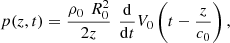 (1) where ρ
0 is the air density and c
0 is the speed of sound.
(1) where ρ
0 is the air density and c
0 is the speed of sound.
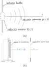 |
Figure 1 Description of the physical model composed of (a) on-axis baffled piston radiation for the evaluation of the sound pressure and (b) conversion of the piston displacement into an equivalent Eulerian velocity source |

The core of this study focuses on the (nonlinear) mapping between the rigid piston displacement and the equivalent Eulerian velocity field V 0(t), as described in Figure 1b. This issue is addressed under the following assumptions:
-
H1 (geometry): The piston displacement ξ(t) is small compared to its radius (|ξ(t)| < ξ max ≪ R 0)
-
H2 (fields equivalence approximation): In the domain Ω = [−ξ max, ξ max], the particle velocity ξ′(t) at the piston position ξ(t) results from the conservative plane wave propagation of an Eulerian velocity field V 0(t) at z = 0
-
H3 (waveform): the piston displacement ξ is a smooth function and no shockwave propagates in Ω
-
H4 (radiation): the piston radiates into a semi-infinite space (no backward wave)
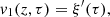
Following (H1–H2–H4), the particle velocity  is described by a forward wave V
0
is described by a forward wave V
0
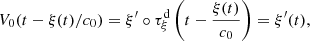
 (2) and satisfies a moving-boundary condition at the piston position that reads
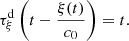
 (3)
(3)
Moreover, condition H3 implies that the Eulerian velocity field V 0 must be a regular function.
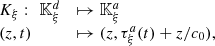
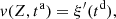
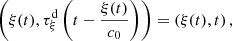
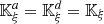
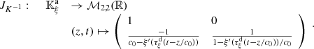
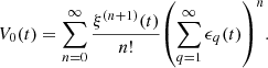
Let us denote  the operator that converts the piston displacement into its equivalent Eulerian velocity (see Fig. 2), such that
 $](/articles/aacus/full_html/2020/01/aacus200002s/aacus200002s-eq7.gif) . This study examines the following problems:
. This study examines the following problems:
 |
Figure 2 Block diagram of the system under consideration, with input |


-
P1 (Direct problem): Is-it possible to derive a solver for
 that satisfies (2)–(3)?
 -
P2 (Inverse problem): What is the corrected displacement ξ c(t) to provide to
 so that its output is the target
  ?
?
The direct problem P1 is tackled in Section 3 and the inverse problem P2 is examined in Section 4.
3 Direct problem: simulation of the Doppler distortion
This section addresses the direct problem (Doppler effect) for smooth excitations: in Section 3.1, an exact solution of the Eulerian velocity V 0 is determined for a linear propagation, based on the method of characteristics; in Section 3.2, a truncated series expansion that approximates the Eulerian velocity V 0 by a closed-form solution is derived for simulation purposes, based on a perturbation method; the distortion is evaluated on the radiated pressure in Section 3.3; finally Section 3.4 includes the influence of nonlinear acoustic wave propagation.
3.1 Method of characteristics
This part addresses the existence and uniqueness of regular solutions of P1, based on the method of characteristics. It provides a regular expression of the velocity waveform V
0 under a necessary and sufficient condition on  -regular functions ξ. In the following,
-
“a” refers to quantities related to the arrival time of the acoustic wave at the observing point,
-
“d” denotes quantities related to the departure time of the wave from the piston position.
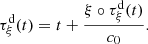
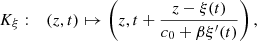
Definition 3.1 (Characteristic)
Let us define the regular functions
 (4)
and
(4)
and
 (5)
where the domain
(5)
where the domain
 and codomain
 are
are
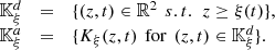 (6)
(6)
The characteristic lines K ξ defined above are depicted in Figure 3. They represent the linear propagation of the acoustic wave over space and time. A departure time t d is mapped to an arrival time t a at a given position Z through K ξ . One should note that
-
the propagation is conservative so that the particle velocity is constant on the characteristic line described by K ξ (r, t d) when z varies, for given a departure time t d. For the boundary condition (3), this observation yields
-
the departure and arrival times are related by
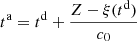 . This can be written using the characteristic equation (6),
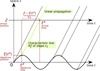 |
Figure 3 Illustration of the mapping from departure coordinates |


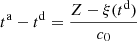
 (7)
(7)
 (8)
(8)
It is clear from these observations that the particle velocity v at any space-time coordinates  can be computed from (7), if the departure time t
d is known. However, equation (8) shows that the existence of t
d is conditionned by the existence of
can be computed from (7), if the departure time t
d is known. However, equation (8) shows that the existence of t
d is conditionned by the existence of  , the reciprocal of K
ξ
. This point is examined in the property detailed in Appendix A, which yields a condition on the Mach number of the piston velocity,
, the reciprocal of K
ξ
. This point is examined in the property detailed in Appendix A, which yields a condition on the Mach number of the piston velocity,
 (9)
(9)
Finally, the solution of P1 is given in Theorem 3.2. It provides the regular waveform V 0, solution of the propagation equation (2) and the boundary condition (3), under the Mach number condition (9).
Theorem 3.2 (Regular solution)
Let
 be a
be a
 -regular function and suppose that the Mach number condition
(9)
is fulfilled. Then the regular solution of
(2)–(3)
is given by the
-regular function and suppose that the Mach number condition
(9)
is fulfilled. Then the regular solution of
(2)–(3)
is given by the
 -regular function
 (10)
where
(10)
where
 is the reciprocal of
 .
.
Proof. From the property detailed in Appendix A,  is a
is a  -diffeormorphism, so that the reciprocal
  exists and is
  -regular. Moreover,
 (11) since (ξ(t), t) is a fixed point of K
ξ
. The reciprocal function
(11) since (ξ(t), t) is a fixed point of K
ξ
. The reciprocal function  can be developped
 (12) where the second component of (12) reads
 (13)
(13)
Finally,
 (14) therefore the regular solution (10) verifies the boundary condition (3). Moreover,
  is
is  -regular because
  and
and  are
are  -regular, which concludes the proof. □
This theorem can be summarized in equations (15) and (16), with the expression of the Eulerian source
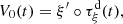 (15) where
  maps the current time t at z = 0 to the departure time of the wave at the piston position, satisfying the implicit equation
 (16)
(16)
The velocity source V 0(t) cannot be directly computed from the piston displacement ξ(t) because of the implicit equation (16). The derivation of a direct solver for (15) and (16) is addressed in the next part.
3.2 Regular perturbation method
A direct solver is established in this subsection, assuming a regular function  and
and  , so that
  from Theorem 3.2. First, function
  is substituted for the
  -regular function
  . Then equations (15) and (16) can be reformulated
 (17)
(17)
 (18)
(18)
Equation (17) highlights that  acts as a perturbation of the standard (linear) solution V
0(t) = ξ′(t).
acts as a perturbation of the standard (linear) solution V
0(t) = ξ′(t).
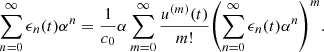
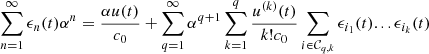
Now the implicit equation (18) is solved using the regular perturbation method. The piston displacement function ξ is marked with an auxiliary amplitude α > 0, so that we define ξ(t) = αu(t). Then we seek a power series solution of  of the form
 (19)
(19)
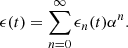
Calculations, developed in Appendix B, yield the exact series solution of the form
 (20)in which each term
  are defined as follows,
 (21)where ξ
(i) stands for the ith derivative of ξ and the ϵ
i
is defined recursively in Appendix B.
(21)where ξ
(i) stands for the ith derivative of ξ and the ϵ
i
is defined recursively in Appendix B.
In the sequel, computation of V 0(t) is carried out by truncating the series at N = 3, that appears sufficient to capture the Doppler distortion effect for typical loudspeaker diaphragm motions. The expression of the truncated series is
 (22)
(22)
The term n = 1 corresponds to the linear solution without taking into account the Doppler effect: the Eulerian field V 0(t) equals the piston velocity. Considering the term n = 2, the product ξ(t)ξ″(t) will be of high amplitude if the piston velocity signal is composed of low frequency components (amplified by ξ) together with high frequencies (amplified by ξ″), therefore generating intermodulation distortion in V 0(t).
A realisation structure of  is drawn from this truncated solution, with input ξ(t) and output V
0(t), depicted in Figure 4. Time-domain simulations are handled for any input signal ξ(t) by choosing appropriate discrete time approximation of the operator
is drawn from this truncated solution, with input ξ(t) and output V
0(t), depicted in Figure 4. Time-domain simulations are handled for any input signal ξ(t) by choosing appropriate discrete time approximation of the operator  .
.
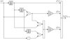 |
Figure 4 Continuous time realisation structure of |

3.3 Evaluation of the Doppler distortion effect
The distortion due to the Doppler effect is evaluated through the computation of the (truncated) Eulerian source (22) and the on-axis pressure field (1) at z = 1 m. First, a piston velocity signal composed of a low-frequency tone at f 0 and a high-frequency tone at f a is chosen, expressed as
 (23)where A, f
0 and f
a
correspond to a realistic high-amplitude loudspeaker motion parameters (see Tab. 1).
(23)where A, f
0 and f
a
correspond to a realistic high-amplitude loudspeaker motion parameters (see Tab. 1).
Simulation parameters used for the Doppler distortion evaluation.
The amplitude spectrum of the acoustic pressure P(f) for the piston velocity signal (23) is depicted in Figure 5, where P(z = 1, f) is the discrete Fourier transform or p(z = 1, t). One should note that the level of the low-frequency f 0 is lower than that of the high-frequency tone f a because of the time derivation of the velocity signal in (1). Two kinds of signal distortion are observed:
-
Harmonic distortion (HD) at frequency 2f 0 = 80 Hz. The level of the harmonic is −56 dB below the fundamental f 0. In the case of loudspeaker diaphragm motion, this effect is often considered as neglectable [6].
-
Intermodulation distortion (IMD) at frequencies f a ± f 0, f a ± 2f 0 and f a ± 3f 0. The low-frequency tone f 0 modulates the high-frequency tone, generating sidelobes around f a = 1 kHz. The first-order intermodulation peaks f a ± f 0 reach −35 dB below the fundamental f a .
 |
Figure 5 Amplitude spectrum of the acoustic pressure for a piston velocity signal composed of a low-frequency tone at |


The above-mentionned intermodulation distortion effect can be seen in the time domain in Figure 6, where the signal p(z = 1, t) (solid line) is represented for a few periods 1/f a . A time shift of the high-frequency waveform is observed, compared to the acoustic pressure without Doppler effect (dashed line). This corresponds to the time-domain version of the frequency modulation caused by the Doppler effect.
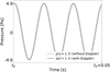 |
Figure 6 Time domain signal |

In order to evaluate the influence of the high-frequency tone on the Doppler distortion, a second input velocity signal is examined, composed of a low-frequency tone at f 0 and a logarithmic chirp whose instantaneous frequency varies between f a and f b . The piston velocity expression reads
 (24)where f
b
and T are defined in Table 1. The spectrograms of the piston velocity signal (24) and the acoustic pressure are depicted respectively in Figures 7 and 8.
(24)where f
b
and T are defined in Table 1. The spectrograms of the piston velocity signal (24) and the acoustic pressure are depicted respectively in Figures 7 and 8.
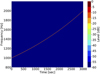 |
Figure 7 Spectrogram of the input piston velocity signal ξ′(t), consisting of a chirp in the range [ |


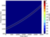 |
Figure 8 Spectrogram of the output acoustic pressure |

![Mathematical equation: $ f\in [{f}_a,{f}_b]$](/articles/aacus/full_html/2020/01/aacus200002s/aacus200002s-eq82.gif)
Only the chirp part of the signal in the range [f
a
, f
b
] is visible on these graphs. Sidelobes are still observed along the rising frequency. Second-order intermodulation products of frequency f ± f
0 are noticed with amplitudes in the range [−35 dB, −25 dB]. Weak third order intermodulation (f ± 2f
0) is also noted. This highlights once again the intermodulation distortion created by the low-frequency tone  . Moreover the sidelobes level clearly increase with the chirp frequency: the first sidelobe f ± f
0 starts at −35 dB at f
a
= 1000 Hz to reach −25 dB at f
b
= 2000 Hz.
. Moreover the sidelobes level clearly increase with the chirp frequency: the first sidelobe f ± f
0 starts at −35 dB at f
a
= 1000 Hz to reach −25 dB at f
b
= 2000 Hz.
This numerical evaluation states that the Doppler effect of a vibrating piston causes mostly intermodulation distortion in the radiated pressure, in agreement with previous studies. This distortion increases with the ratio f max/f min, where f min and f max are respectively the minimum and maximum frequency of excitation. For a realistic loudspeaker diaphragm motion, it is shown that this effect can potentially produce sound corruption at −25 dB below the unaltered pressure signal.
3.4 Nonlinear wave propagation effect
Several authors [1, 10] have pointed out that the moving-boundary (Doppler) effect should be tackled together with the nonlinear propagation phenomenon, since both appear at large diaphragm displacements. This section briefly investigates this coupling by substituting the linear propagation in H2 for the inviscid Burger’s equation, describing the nonlinear propagation of progressive plane waves,
 (25)where β is a coefficient derived from the nonlinear relationship between pressure and air density. This equation can be solved by using the method of characteristics as in Section 3.1. In that case, the characteristic reads
 (26)where the term 1/(c
0 + βξ′(t)) stands for the nonlinear propagation effect: the propagation speed differs from c
0 and is higher for high-amplitude waves. The moving-boundary is still taken into account by the term z − ξ(t). The existence of
(26)where the term 1/(c
0 + βξ′(t)) stands for the nonlinear propagation effect: the propagation speed differs from c
0 and is higher for high-amplitude waves. The moving-boundary is still taken into account by the term z − ξ(t). The existence of  is limited (i) in space by the nonlinear propagation (z should be small enough so that no shockwave appears) and (ii) in amplitude by the Mach number condition as in (9).
A formal series solution for the particle velocity v(z, t) is derived by applying a perturbation method similar to Section 3.2. The three first orders are listed below:
 (27)
(27)
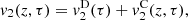 (28)
(28)
 (29)where τ = t − z/c
0,
(29)where τ = t − z/c
0,  and
and  correspond to the terms solely due to the Doppler effect (defined in (22)) and the convective terms
  and
and  are
are
 (30)
(30)
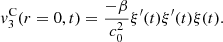
![Mathematical equation: $$ \begin{aligned}{v}_3^{\mathrm{C}}(z,\tau )&=\frac{-\beta }{{c}_0^2}{\xi }^{\prime }\left(\tau \right){\xi }^{\prime}(\tau )\xi (\tau ){c}+\frac{{\beta z}}{{c}_0^3}\left[{\xi }^{{\prime\prime\prime}}\left(\tau \right){\xi }^{\prime}(\tau )\xi (\tau )\right.\\ &\quad\left.+({\xi }^{\prime\prime}(\tau ))^2\xi (\tau )+\left(1-\beta \right){\xi }^{\prime\prime }(\tau )({\xi }^{\prime\prime }(\tau ))^2\right]\\ &\quad+\frac{{\beta }^2{z}^2}{{c}_0^4}\left[({\xi }^{\prime\prime }\left(\tau \right))^2{\xi }^{\prime}(\tau )+\frac{{\xi }^{{\prime\prime\prime}}(\tau )({\xi }^{\prime}(\tau ))^2}{2}\right],\end{aligned} $$](/articles/aacus/full_html/2020/01/aacus200002s/aacus200002s-eq95.gif) (31)
(31)
The contribution of the convection can be separated from the Doppler effect up to the order 3, as described in equations (27)–(29). One should note that this separation is not possible for higher order terms since both effects will be coupled. Moreover the convective terms at z = 0 yield
 (32)
(32)
 (33)
(33)
It appears that orders 1 and 2 does not influence the equivalent Eulerian source  at z = 0. However the third order term
  has a nonzero value at z = 0. This corresponds to the influence of nonlinear propagation in the domain Ω = [−ξ
max, ξ
max], that alternates the equivalent Eulerian source at z = 0 calculated in (22). Therefore the Doppler effect can be treated independently from the nonlinear propagation at orders 1 and 2, but higher orders require consideration of both effects coupled. In the following part, the anti-Doppler system is derived from third order expansion of V
0(t) presented in Section 3.2, thus neglecting the term (33) introduced by the nonlinear propagation.
has a nonzero value at z = 0. This corresponds to the influence of nonlinear propagation in the domain Ω = [−ξ
max, ξ
max], that alternates the equivalent Eulerian source at z = 0 calculated in (22). Therefore the Doppler effect can be treated independently from the nonlinear propagation at orders 1 and 2, but higher orders require consideration of both effects coupled. In the following part, the anti-Doppler system is derived from third order expansion of V
0(t) presented in Section 3.2, thus neglecting the term (33) introduced by the nonlinear propagation.
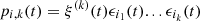
4 Inverse problem: anti-Doppler system
This section presents the derivation of a corrector  that provides a diaphragm displacement ξ
c
(t) compensating for the Doppler effect. This feed-forward controller relies on the design of a pre-inverse system, as described in Figure 9. First, the operator
that provides a diaphragm displacement ξ
c
(t) compensating for the Doppler effect. This feed-forward controller relies on the design of a pre-inverse system, as described in Figure 9. First, the operator  is recasted into the Volterra series formalism in Section 4.1, for which pre-inversion methods exist and are easily tractable [13]. Then a realisation structure of
  is built from the calculated pre-inverse kernels in Section 4.2.
 |
Figure 9 Description of the pre-inverse system |


4.1 Volterra series formulation
Proposition 4.1
The system
 admits a representation into Volterra series and its transfer kernels are given by
 (34)
where
(34)
where
 (35)
and
(35)
and
 ,
,
 .
.
The proof is given in Appendix C. The three first kernels calculated from this proposition are listed below:
 (36)
(36)
 (37)
(37)
 (38)
(38)
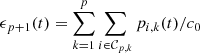
4.2 Third-order corrector calculation
The purpose of the anti-Doppler filter is to reshape the diaphragm displacement waveform ξ(t) into another displacement ξ c (t) in order to reach the following target Eulerian velocity field,
 (39)
(39)
The pre-inverse system presented in Figure 9 is calculated so that the tandem system  of input
  must be equal to the identity. This property is translated into the Volterra series formalism by
 (40)
(40)
Moreover, higher order terms of the series composition must vanish, yielding one equation per order. Solving recursively for n = 1, 2, 3 yields
 (41)
(41)
 (42)
(42)
 (43)
(43)
The realisation structure of (41)–(43) is presented in Figure 10. A prior integration of V
0(t) = ξ′(t) is assumed, so that ξ(t) is the input of  . This correction algorithm is also decomposed into orders of homogeneous degree, where for instance ξ
c1(t) = ξ(t) is the contribution from the first order.
. This correction algorithm is also decomposed into orders of homogeneous degree, where for instance ξ
c1(t) = ξ(t) is the contribution from the first order.
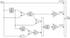 |
Figure 10 Continuous time realisation structure of |


Note that the second-order term
![Mathematical equation: $$ \begin{array}{ll}{\xi }_{c2}(t)& =-\frac{1}{{c}_0}{\int }_0^t {\xi }^{\mathrm{\prime }}(t)\xi (t)\mathrm{d}t\\ & =\frac{1}{{c}_0}\left({\int }_0^t [{\xi }^\mathrm{\prime}(t){]}^2\mathrm{d}t-\xi (t){\xi }^\mathrm{\prime}(t)\right)\end{array} $$](/articles/aacus/full_html/2020/01/aacus200002s/aacus200002s-eq126.gif) (44)is not centered on zero and constantly increases with time due to the integral of [ξ′(t)]2. A similar divergence can be observed for the third-order term. This problem, illustrated in Figure 11, can be interpreted as follows: the particle velocity generated by the moving piston is slightly more compressed for positive values and relaxed for negative values (see top-right picture in Fig. 11), leading to a signal assymetry and thus a non-zero (negative) mean value. Therefore the required diaphragm displacement ξ
c
(t) to perfectly compensate for the Doppler effect must constantly move toward the listener (see down-left picture in Fig. 11). To get around this problem, another corrector
(44)is not centered on zero and constantly increases with time due to the integral of [ξ′(t)]2. A similar divergence can be observed for the third-order term. This problem, illustrated in Figure 11, can be interpreted as follows: the particle velocity generated by the moving piston is slightly more compressed for positive values and relaxed for negative values (see top-right picture in Fig. 11), leading to a signal assymetry and thus a non-zero (negative) mean value. Therefore the required diaphragm displacement ξ
c
(t) to perfectly compensate for the Doppler effect must constantly move toward the listener (see down-left picture in Fig. 11). To get around this problem, another corrector  is proposed, that substitutes the perfect integrator
  in the Laplace domain for 1/(s + 2πf
c
), where f
c
is below the lowest frequency of interest. The impact of this substitution is evaluated on the orders 1 and 2 by connecting in tandem
in the Laplace domain for 1/(s + 2πf
c
), where f
c
is below the lowest frequency of interest. The impact of this substitution is evaluated on the orders 1 and 2 by connecting in tandem  and
and  in equations (45) and (46).
-
The identity is retrieved (
 if n = 1 and
  for n = 2) by setting a = 0.
 -
The composition
 behaves like a gain of
  for frequencies greater than f
c
.
for frequencies greater than f
c
. -
The composition
 is equivalent to the product of two filters s/(s + 2πf
c
), connected in tandem with an integrator 1/(s + 2πf
c
) and a gain of −2πf
c
. The result of this composition is very close to
is equivalent to the product of two filters s/(s + 2πf
c
), connected in tandem with an integrator 1/(s + 2πf
c
) and a gain of −2πf
c
. The result of this composition is very close to  for frequencies greater than f
c
.
for frequencies greater than f
c
.
 (45)
(45)
 (46)
(46)
 |
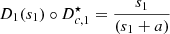
Figure 11 Illustration of the (slow) divergence of the displacement signal for a centered target Eulerian field. The centered displacement signal |


Similar observations can be made by evaluating the third order. It can be concluded that  tends to equal
  for frequencies higher than
  , therefore restoring the exact correction for sufficiently high frequencies.
4.3 Numerical evaluation of the corrector
The evaluation of the corrector is carried out with the same piston velocity signal as in the previous Section 3, composed of a low-frequency tone and a rising chirp. The cutoff frequency of  is set to
  Hz and the numerical integration is achieved by the bilinear transform of
  . A complete block diagram of the correction evaluation is presented in Figure 12: the targeted Eulerian field is sent to the corrector
  that generates a corrected piston displacement
  . Then the Eulerian source
  is calculated through
  and the acoustic pressure is evaluated at z = 1 m by (1).
 |
Figure 12 Block diagram of the corrector evaluation, with the target Eulerian field as input |


Spectrogram of the corrected acoustic pressure  , presented in Figure 13, should be compared to the case without correction in Figure 8. Second order intermodulation is now below −36 dB (compared to −25 dB without correction) and third order is no longer visible.
 |
Figure 13 Spectrogram of the acoustic pressure |


Finally, an intermodulation factor is evaluated at the swept sine frequency  from the following formula,
![Mathematical equation: $$ {{IMD}}_P(f)=100\frac{\sqrt{\frac{1}{4}\sum_{n=1}^2 \left[P(f+n{f}_0{)}^2+P(f-n{f}_0{)}^2\right]}}{|P(f)|}, $$](/articles/aacus/full_html/2020/01/aacus200002s/aacus200002s-eq159.gif) (47)where
(47)where  is the discrete Fourier transform of the acoustic pressure
  . This factor is calculated at various ratio
  , with and without correction of the piston displacement.
The results, presented in Figure 14, confirms the increase of intermodulation distortion with frequency: the case without correction reaches 15% of IMD for  . For
. For  , which corresponds to a realistic case
  Hz and f = 2 kHz, the IMD is about 7.5%. The correction algorithm
  maintains the intermodulation level below 4%. The slight loss of efficiency of
  with frequency is due to (i) the truncation at order
  and (ii) the phase and amplitude limitations of the implemented differentiator filter.
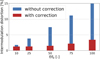 |
Figure 14 Evolution of the intermodulation distortion |


5 Conclusion
The influence of the Doppler effect induced by a vibrating source has been investigated in terms of intermodulation distortion, based on the truncation of an exact series expansion that generates an equivalent Eulerian velocity field. The sound artefact generated by this nonlinear phenomenon increases with the distance between the highest and the lowest frequencies of the source signal.
Distortions can be expected up to 7.5% for diaphragm displacements with a wide frequency content (typically [40 Hz, 2 kHz]) and large amplitudes (a few millimeters). In this situation, truncating the series expansion at order 3 is sufficient to represent this distortion effect with a good accuracy. Also, the nonlinear propagation (due to convection) has been examined: this effect only appears from order 3. More precisely, compared to the Doppler alone, the convection effect only modifies one coefficient of the third order contribution.
In addition, an algorithm to compensate for this effect while preserving a centered version of the membrane displacement has been proposed. The solution is derived by inverting the series of the direct problem and replacing each time-integrator by a “band-limited integrator”. Numerical tests show that this solution yields a satisfying distortion reduction.
A future work is concerned with the experimental validation of the proposed Doppler system on loudspeakers. Another one will be devoted to the validation of the anti-Doppler system, through its combination with correction techniques to reject the driver electromechanical nonlinearities.
Conflict of interest
Authors declared no conflict of interests.
References
- D.W. van Wulfften Palthe: Doppler effect in loudspeakers. Acustica 28 (1973) 5–11. [Google Scholar]
- P.W. Klipsch: Modulation distortion in loudspeakers. Journal of the Society of Motion Picture Engineers 17 (1969) 194–206. [Google Scholar]
- E. Villchur, R.F. Allison: The audibility of Doppler distortion in loudspeakers. The Journal of the Acoustical Society of America 68 (1980) 1561–1569. [Google Scholar]
- A.J. Kaizer: Modeling of the nonlinear response of an electrodynamic loudspeaker by a Volterra series expansion. Journal of the Audio Engineering Society 35 (1987) 421–433. [Google Scholar]
- W. Klippel: Prediction of speaker performance at high amplitudes. Audio Engineering Society Convention 111. Audio Engineering Society, New York, NY, 2001. [Google Scholar]
- W. Klippel: Tutorial: Loudspeaker nonlinearities – Causes, parameters, symptoms. Journal of the Audio Engineering Society 54 (2006) 907–939. [Google Scholar]
- G.L. Beers, H. Belar: Frequency modulation distortion in loudspeakers. Journal of the Society of Motion Picture Engineers 40 (1943) 207–221. [CrossRef] [Google Scholar]
- S. Braun: Time-domain formulation of the Doppler effect. The Journal of the Acoustical Society of America 59 (1976) 1495–1497. [Google Scholar]
- H.J. Butterweck: About the Doppler effect in acoustic radiation from loudspeakers. Acustica 63 (1987) 77–79. [Google Scholar]
- B. Zóltogórski: Moving boundary conditions and nonlinear propagation as sources of nonlinear distortions in loudspeakers, Journal of the Audio Engineering Society 41 (1993) 691–700. [Google Scholar]
- W. Klippel: The mirror filter – a new basis for reducing nonlinear distortion and equalizing response in woofer systems. Journal of the Audio Engineering Society 40 (1992) 675–691. [Google Scholar]
- P.M. Morse, K.U. Ingard: Theoretical Acoustics. Princeton University Press, NJ, USA, 1986, p. 388. [Google Scholar]
- M. Schetzen: Theory of pth-order inverses of nonlinear systems. IEEE Transactions on Circuits and Systems 23 (1976) 285–291. [CrossRef] [Google Scholar]
Appendix A
Property 1:  is a diffeomorphism
Property A.1 ( is a
is a  -diffeomorphism)
Let
 be a
be a
 -regular function that satisfies the condition 9 on the Mach number. If function
 is also
 -regular with
 , then
-
 is a
is a
 -regular diffeomorphism. Consequently the functions
 and
and
![Mathematical equation: $ {\tau }_{\xi }^d=[{\tau }_{\xi }^a{]}^{-1}$](/articles/aacus/full_html/2020/01/aacus200002s/aacus200002s-eq184.gif) exist and are
exist and are
 -regular,
-
 .
.
Proof. (i) Bijection. By construction of the image set  (see (6)),
  is a surjective function. Moreover
  is
is  -regular, so that
  and then
  are also
  -regular functions. For all
  , the Jacobian of
  is given by
 in which
  is strictly positive from (9), therefore
  is bijective.
(ii) Diffeomorphism. Now let  and consider
  -regular. Then,
  exists and can be expressed as
 (A1)where
  is the reciprocal of
  . The Jacobian of
  is given by
 (A2)
(A2)
Now, we prove by induction that  is
is  -regular for
  .
.
• Case
 :
:
 .
.
-
From (4),
 is
is  -regular, so that
  exists and is continuous. Then the Jacobian
  defined in (A2) is a continuous function, so that
  and then
  are
are  -regular.
• Case
 : If
: If
 is
is
 -regular, then
 is
is
 -regular.
-
From (A2), the Jacobian
 is
is  -regular. Therefore and
 are
are  -regular, which proves that
  is a diffeomorphism.
Moreover,  proves that the codomain
  is also bounded by the fixed point
  , leading to
  . □
. □
Appendix B
Derivation of the perturbation method
Injecting (19) into (18) yields
 (B1)where function u can be expanded into Taylor series at point t, leading to
 (B2)
(B2)
The power series composition at the right-hand side is simplified as follows,
 (B3)where
  is the set of compositions of
  into
into  parts. Finally, equating (B3) for each power of
  yields the following recursive relation, for all
  ,
,
 (B4)where the amplitude
  is set to
  , so that
  .
.
Now that (18) is solved, (17) can be written
 (B5)where ξ′ can be expanded into Taylor series at point t
 (B6)
(B6)
Appendix C
Proof of Proposition 4.1
Proof. The formula (35) is proven by induction.
• Case
 :
:  .
.
The proof is straightforward since 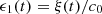 , so that its associated transfer kernel is
  .
.
• Case
 : if
: if  is true, then
 is true.
From its construction using the regular perturbation method,  is a homogeneous multivariate polynomial of degree
  , so that its associated transfer kernel only consists of order
  . Thus, the transfer kernel of following product
 (C1)is given by
 (C2)
(C2)
Therefore the transfer kernel associated with
 (C3)is
 (C4)that concludes the proof by induction.
The transfer kernels  are derived similarly. □
Cite this article as: T. Lebrun and T. Hélie. 2020. Correction of the Doppler distortion generated by a vibrating baffled piston. Acta Acustica, 4, 2.
All Tables
All Figures
|
Figure 1 Description of the physical model composed of (a) on-axis baffled piston radiation for the evaluation of the sound pressure and (b) conversion of the piston displacement into an equivalent Eulerian velocity source |
| In the text | |
|
Figure 2 Block diagram of the system under consideration, with input |
| In the text | |
|
Figure 3 Illustration of the mapping from departure coordinates |
| In the text | |
|
Figure 4 Continuous time realisation structure of |
| In the text | |
|
Figure 5 Amplitude spectrum of the acoustic pressure for a piston velocity signal composed of a low-frequency tone at |
| In the text | |
|
Figure 6 Time domain signal |
| In the text | |
|
Figure 7 Spectrogram of the input piston velocity signal ξ′(t), consisting of a chirp in the range [ |
| In the text | |
|
Figure 8 Spectrogram of the output acoustic pressure |
| In the text | |
|
Figure 9 Description of the pre-inverse system |
| In the text | |
|
Figure 10 Continuous time realisation structure of |
| In the text | |
|
Figure 11 Illustration of the (slow) divergence of the displacement signal for a centered target Eulerian field. The centered displacement signal |
| In the text | |
|
Figure 12 Block diagram of the corrector evaluation, with the target Eulerian field as input |
| In the text | |
|
Figure 13 Spectrogram of the acoustic pressure |
| In the text | |
|
Figure 14 Evolution of the intermodulation distortion |
| In the text | |
Current usage metrics show cumulative count of Article Views (full-text article views including HTML views, PDF and ePub downloads, according to the available data) and Abstracts Views on Vision4Press platform.
Data correspond to usage on the plateform after 2015. The current usage metrics is available 48-96 hours after online publication and is updated daily on week days.
Initial download of the metrics may take a while.