| Issue |
Acta Acust.
Volume 4, Number 5, 2020
|
|
|---|---|---|
| Article Number | 17 | |
| Number of page(s) | 9 | |
| Section | Underwater Sound | |
| DOI | https://doi.org/10.1051/aacus/2020017 | |
| Published online | 02 October 2020 | |
Scientific Article
A miniaturized acoustic vector sensor with PIN-PMN-PT single crystal cantilever beam accelerometers
1
Agency for Defense Development, POB 18, 40, Baekgu-ro, Jinhae-gu, Changwon-si, Gyeongsangnam-do 51678, South Korea
2
School of Mechanical Engineering, Pusan National University, Busandaehak-ro 63, Geumjeong-gu, Busan 46241, South Korea
* Corresponding author: This email address is being protected from spambots. You need JavaScript enabled to view it.
Received:
13
April
2020
Accepted:
28
August
2020
Abstract
Directional sound detection using vector sensors rather than large hydrophone arrays is highly advantageous for target detection in SONAR. However, developing highly sensitive and compact vector sensors for use in a system whose size is limited has been a challenging issue. In this paper, we describe a miniaturized acoustic vector sensor with piezoelectric single crystal accelerometers for the application in towed line arrays. A mass-loaded cantilever beam accelerometer with a [011] poled PIN-PMN-PT single crystal shows a better signal-to-noise ratio compared to accelerometers with other piezoelectric materials because of its superior piezoelectric properties in the 32 direction. We suggested a sufficiently compact vector sensor by using a cylindrical hydrophone with 10 mm in diameter as a housing of the single crystal accelerometers. Two single crystal accelerometers were orthogonally mounted inside the cylindrical hydrophone to detect direction of sound in the transverse plane of the line array. The receiving voltage sensitivity of the accelerometers and hydrophone was −199 and −196 dB, respectively, at 3 kHz. The directional cardioid beams generated by summing the omnidirectional beam from the hydrophone and the dipole beam from the accelerometers were validated over the entire operating frequency.
Key words: Inertial vector sensors / Cantilever beam accelerometers / [011] poled PIN-PMN-PT / Directional hydrophones / Towed line arrays
© Y. Cho et al., Published by EDP Sciences, 2020
 This is an Open Access article distributed under the terms of the Creative Commons Attribution License (https://creativecommons.org/licenses/by/4.0), which permits unrestricted use, distribution, and reproduction in any medium, provided the original work is properly cited.
1 Introduction
Directional sound detection using large arrays of single hydrophones has been widely used for target detection in sonar. Towed line arrays, a linear line of hydrophone elements deployed by submarines and surface vessels, provide bearing of the targets using directional beam along the line. However, on the plane perpendicular to the line, the axial beam is symmetrical, leading to left-right ambiguity [1, 2]. Vector sensors measure both acoustic particle velocity and pressure amplitude and thus measure the direction of the incoming acoustic wave without constructing large hydrophone arrays. Applying vector sensors to towed line arrays thus provides the discrimination between left and right [3–6].
There are several types of vector sensors that can be used in towed line arrays. Pressure gradient vector sensors measure the pressure differences between multiple pressure-sensing hydrophones for directional sound detection. Arranging three or four elements in the transverse plane of the line array [7–9], as well as twin-line arrays [10], has been investigated for pressure gradient vector sensors of towed line arrays. However, those line arrays must have a relatively large radius since their performance depends on the gap between the pressure-sensing hydrophones [11, 12].
Inertial vector sensors directly measure sensor body motion induced by acoustic waves by using an accelerometer or a geophone [11, 12]. Because such vector sensors inherently measure the point value of the velocity, they can be small enough for use in thin line arrays. However, there are some difficulties in applying the inertial vector sensors to sonar [12, 13]. The inertial vector sensors should be lightweight close to neutral buoyancy, for sensitive body motion induced by an acoustic wave. Also, the frequency-dependent sensitivity of the accelerometers with 6 dB per octave slope below resonance results in insensitive low-frequency response. A highly sensitive accelerometer with lightweight housing is thus required for low-frequency wave detection using inertial vector sensors.
Relaxor-ferroelectric single crystals, such as lead magnesium niobate-lead titanate (PMN-PT) and lead zinc niobate-lead titanate (PZN-PT) can provide significant advantages for underwater acoustic transducers because their piezoelectric properties are superior to those of polycrystalline ceramics such as lead zirconate titanate (PZT) [14, 15]. Acoustic projectors with single crystals can have high source levels in broadband frequency because single crystals have high electromechanical coupling coefficients (k ~ 0.9) and large piezoelectric constants (d ≥ 1200 pC/N). When used in acoustic receivers, the large piezoelectric d and g constants and high coupling coefficients of such crystals enhance the signal-to-noise ratio and broaden the bandwidth [16].
In this paper, we develop a miniaturized acoustic vector sensor with piezoelectric single crystal accelerometers for application in towed line arrays. A mass-loaded cantilever beam accelerometer with a [011] poled PIN-PMN-PT single crystal shows a better signal-to-noise ratio than accelerometers with other piezoelectric materials because of its superior piezoelectric properties in the 32 direction. By using a cylindrical PZT hydrophone as a housing for the accelerometers, we propose a miniaturized vector sensor usable in towed line arrays. The vector sensor was designed and built to have two single crystal accelerometers that are mounted orthogonally inside the cylindrical hydrophone. The omnidirectional hydrophone and the dipole accelerometers were combined to generate a cardioid directivity of the vector sensor.
The background and motivation for this research were described in Section 1 above. Section 2 describes a theoretical analysis of the vector sensor and the cantilever beam accelerometer used in it. The sensor design and fabrication are described in Section 3. The test and conclusions are presented in Sections 4 and 5, respectively.
2 Theoretical analysis
2.1 The cantilever beam accelerometer
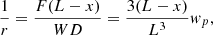
A cantilever beam accelerometer generally has a piezoelectric unimorph or bimorph structure, with a proof mass at the tip to measure base vibration. High compliance of the cantilever beam structure allows highly sensitive measurement of the base motion and a light proof mass to have a desirable resonance frequency. Also, the simple structure with a compact size has advantages [17, 18]. Figure 1a shows a bimorph cantilever beam accelerometer with a proof mass at the tip and a piezoelectric layer on top and bottom of the elastic substrate. The curvature of cantilever r under point force F is:
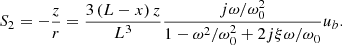
 (1)where L and W are the cantilever length and width, respectively. w is the transverse deflection of the cantilever along its length. The bending moment of the cantilever at x is given by M = F(L − x). D is the bending modulus of the cantilever [19]:
 (2)where E
s and t
s are the Young’s modulus and thickness of the substrate, and E
p and t
p are the Young’s modulus and thickness of the piezoelectric layer. Given the boundary conditions of the clamped base (w
b
= 0,
(2)where E
s and t
s are the Young’s modulus and thickness of the substrate, and E
p and t
p are the Young’s modulus and thickness of the piezoelectric layer. Given the boundary conditions of the clamped base (w
b
= 0, ), the transverse deflection of the cantilever is obtained by integrating equation (1) over length:
 (3)
(3)
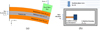 |
Figure 1 (a) Bimorph cantilever beam accelerometer under base excitation, and (b) Vector sensor with cantilever beam accelerometers and a cylindrical housing. |
The curvature of cantilever is calculated using equations (1) and (3):
 (4)where w
p
is the deflection of the proof mass at the end of the cantilever. The equivalent stiffness of the cantilever is:
(4)where w
p
is the deflection of the proof mass at the end of the cantilever. The equivalent stiffness of the cantilever is:
 (5)
(5)
The accelerometers measure the base motion of the housing induced by an acoustic wave. The equation of motion for the cantilever beam under base excitation u b is:
 (6)where a and u are the acceleration and velocity of the cantilever, respectively. The relative deflection w′ between the clamped base (x = 0) and the tip (x = L) is calculated by solving equation (7):
 (7)where
  is the resonance frequency of the cantilever and
  is the mechanical damping coefficient.
The strain of the cantilever along its length is obtained using equations (3), (4), and (7):
 (8)
(8)
The voltage sensitivity with respect to base excitation can be calculated using the constitutive equations of the piezoelectric layer:
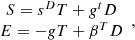 (9)where S is the mechanical strain, T is the mechanical stress, D is the electric displacement, and E is the electric field. Under the open-circuit receiver conditions, the electric displacement D
3 = 0. As the sides of the cantilever are free to move and the lateral dimensions are small, the lateral stresses T
1 and T
3 are both zero throughout the cantilever. The constitutive equations, equation (9) reduces to:
(9)where S is the mechanical strain, T is the mechanical stress, D is the electric displacement, and E is the electric field. Under the open-circuit receiver conditions, the electric displacement D
3 = 0. As the sides of the cantilever are free to move and the lateral dimensions are small, the lateral stresses T
1 and T
3 are both zero throughout the cantilever. The constitutive equations, equation (9) reduces to:
 (10)
(10)
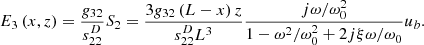
The electric field E 3 (x, z) of the piezoelectric layer is obtained using equations (8) and (10):
 (11)
(11)
By integrating the electric field E 3 (x, z) through the piezoelectric thickness z, the voltage at any x is:
 (12)
(12)
Redistribution of the induced electric charge creates a uniform electrical potential over the electrode of the piezoelectric layer. The voltage at the electrode is the average V(x) over the length L of the piezoelectric layer:
 (13)
(13)
The voltage sensitivity with respect to the base excitation is:
 (14)
(14)
2.2 The vector sensor
An accelerometer-based vector sensor has a housing within which accelerometers are mounted. Figure 1b shows a vector sensor with a cantilever beam accelerometer mounted within a cylindrical housing of cross-sectional area A
c
, length L
c
, and total mass m. The translation housing velocity u
b
induced by an incident plane wave with acoustic particle velocity u
i
, pressure amplitude  , and incident angle
  is [20]:
 (15)where B = ρA
c
L
c
/m is the buoyancy of the vector sensor and ρ and c are the water density, and speed of sound. The base velocity u
b
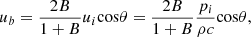
is a function of system buoyancy and the pressure amplitude, and equals the acoustic particle velocity when the vector sensor is neutrally buoyant (B = 1). The accelerometer exhibits a dipole directivity pattern, because the base velocity is proportional to the cosine of the pressure angle of incidence θ. The pressure sensitivity of the cantilever beam accelerometer on its acoustic axis is obtained from equations (14) and (15):
(15)where B = ρA
c
L
c
/m is the buoyancy of the vector sensor and ρ and c are the water density, and speed of sound. The base velocity u
b
is a function of system buoyancy and the pressure amplitude, and equals the acoustic particle velocity when the vector sensor is neutrally buoyant (B = 1). The accelerometer exhibits a dipole directivity pattern, because the base velocity is proportional to the cosine of the pressure angle of incidence θ. The pressure sensitivity of the cantilever beam accelerometer on its acoustic axis is obtained from equations (14) and (15):
 (16)
(16)
If the frequency is well below the resonance frequency, equation (16) becomes:
 (17)
(17)
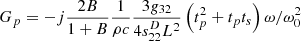
2.3 The figure of merit
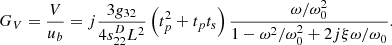
A high sensitivity with a low noise level are among the most important design issues of the vector sensors for sonar. The internal noise level of the sensor is generally proportional to the electrical input impedance [11]. The signal-to-noise is thus the square of the sensitivity divided by the input electrical impedance. The signal-to-noise ratio of a vector sensor with a cantilever beam accelerometer at frequencies well below the resonance frequency is:
 (18)where the free capacitance C
f
= ε
33
A
p
L
p
/t
p
. The figure of merit (FOM), which depends on the properties of the piezoelectric material, can be defined as:
(18)where the free capacitance C
f
= ε
33
A
p
L
p
/t
p
. The figure of merit (FOM), which depends on the properties of the piezoelectric material, can be defined as:
 (19)
(19)
The FOM of vector sensors for various piezoelectric materials are compared in Table 1. Relaxor-ferroelectric single crystals of [0 1 1] poled PIN-PMN-PT and [0 0 1] poled PIN-PMN-PT, and the polycrystalline ceramics of PZT 4 and PZT 5H, are included in the table. Piezoelectric single crystals, especially [0 1 1] poled PIN-PMN-PT, exhibit significantly greater piezoelectric d and g coefficients in the 32 direction compared to polycrystalline ceramics. [0 1 1] poled PIN-PMN-PT thus shows more than three-fold higher sensitivity and 20-fold higher signal-to-noise ratio compared sensors with other piezoelectric materials. Despite the low piezoelectric coefficients, PZT 4 exhibits the next-best sensitivity and signal-to-noise ratio, because its compliance is relatively small.
Figure of merit for vector sensors containing piezoelectric materials: [0 1 1] poled PIN-PMN-PT, [0 0 1] poled PIN-PMN-PT, PZT 5H, and PZT4.
The pressure sensitivity and signal-to-noise ratio of a bimorph cantilever beam vector sensor for various piezoelectric materials is plotted against frequency in Figure 2. Since the response around the resonance frequency is closely related with damping rather than piezoelectric material properties, the sensitivity and signal-to-noise ratio are calculated with low-frequency assumption by using equations (17) and (18). The cantilever beam is 4.0 mm in width and 7.0 mm in length. The thickness of the piezoelectric layer and the elastic steel substrate are 0.4 and 0.3 mm, respectively. The proof mass is determined to have a resonance frequency of 4 kHz. The calculated sensitivities in Figure 2a are proportional to the frequency with a +6-dB per octave slope. The vector sensor with [0 1 1] poled PIN-PMN-PT single crystal has high sensitivity by over 10 dB compared to other piezoelectric materials. The calculated signal-to-noise ratio in Figure 2b is proportional to the f 1.5 with 9 dB per octave slope. The vector sensor with [0 1 1] poled PIN-PMN-PT single crystal has high signal-to-noise ratio by over 13 dB compared to other piezoelectric materials. A single crystal of [0 1 1] poled PIN-PMN-PT shows significant increase of both sensitivity and signal-to-noise ratio of the cantilever beam vector sensor.
 |
Figure 2 (a) Pressure sensitivity and (b) signal-to-noise ratio of a cantilever beam vector sensor containing various piezoelectric materials: [011] poled PIN-PMN-PT, [0 0 1] poled PIN-PMN-PT, PZT 5H, and PZT4. |
3 Design and fabrication
Section 2 showed that a vector sensor with a weight close to neutral buoyancy is important to have a freely moving body with respect to incoming acoustic waves. Also, vector sensors should be sufficiently compact for being usable in towed line arrays whose diameter size is limited. Towed line arrays generally use cylindrical PZT hydrophones to measure the pressure amplitude, because of their high sensitivity, simple structure and reliability in deep sea operations. In this paper, we suggest to use a cylindrical hydrophone as the housing of the single crystal accelerometers for a sufficiently compact vector sensor usable in towed line arrays.
Figure 3a shows a bimorph cantilever beam accelerometer with single crystal piezoelectric layers attached to the top and bottom of the steel substrate. Two single crystal layers are connected in parallel to increase the capacitance, since the noise level of the vector sensor is inversely proportional to the capacitance. The length of cantilever beam is 7 mm. The thickness of the piezoelectric layer and the elastic steel substrate are 0.4 and 0.3 mm, respectively. The cantilever beam accelerometers are designed to have a resonance frequency of 4 kHz with a tungsten proof mass at the tip. A trapezoidal cantilever beam was chosen in order to reduce the off-axis sensitivity while maintaining on-axis sensitivity. High horizontal stiffness of the trapezoidal cantilever beam can reduce the vibration amplitude against the off-axis excitation. Figure 3b shows a vector sensor with cylindrical hydrophone and cantilever beam accelerometers. Two cantilever beam accelerometers are mounted orthogonally on the endcaps of a cylindrical PZT-4 hydrophone. The cylindrical hydrophone has diameter and length of 10 and 20 mm, respectively. The hydrophone and the accelerometers are vibrationally isolated using a decoupler (corprene). The total mass of the vector sensor is about 6.4 g.
 |
Figure 3 The vector sensor design: (a) Bimorph cantilever beam accelerometer clamped by an endcap, and (b) vector sensor with cylindrical hydrophone and cantilever beam accelerometers mounted inside the hydrophone. |
Figure 4 shows the fabrication process of the vector sensor. [0 1 1] poled PIN-PMN-PT (IBULE photonics1) crystals are diced into the desired dimensions. Single crystal layers are attached to the top and bottom of the steel substrate and a proof mass is attached to the cantilever tip in the accelerometer assembly process. The base of the cantilevers is clamped with the insulation layers at the endcaps. Two cantilevers are mounted orthogonally at both ends of the hydrophone in the vector sensor assembly process. The entire assembly was waterproofed with polyurethane.
 |
Figure 4 Fabrication process of the vector sensor. |
4 Test and evaluation
4.1 Vibration test
Figure 5 shows the experimental setup for vibration testing of the vector sensor. The sensor and a reference accelerometer (B&K 4382) were mounted on a vibration exciter (B&K 4809) using a clamping jig. A sine wave signal was generated by a function generator (Agilent 33522A), amplified by a power amplifier (NF HSA4052), and fed into the exciter to generate vibrations in the desired directions. The voltage generated by the accelerometers and hydrophone was measured using a dynamic signal analyzer (SRS SR785).
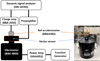 |
Figure 5 Experimental setup for vibration testing of the vector sensor. |
Figure 6 shows the measured acceleration sensitivity of the accelerometers and hydrophone in the directions of the acoustic axes of (a) accelerometer #1 and (b) accelerometer #2. The resonance frequencies of accelerometer #1 and #2 are measured to be 4.1 kHz and 4.2 kHz, respectively. The frequency response of the accelerometers presents a gentle slope below the resonance frequencies. Since the frequency range of interest is not well below the resonance, the mass and damping effect of the accelerometers cause a gentle slope, rather than the flat response expected in the theoretical model. The frequency response of the accelerometers shows a roll-off response below about 400 Hz because a high-pass noise filter is used in pre-amplifiers of the accelerometers. The sensitivity of the accelerometers on the acoustic axis is about 16 dB higher than on the off-axis. The hydrophone shows considerably lower sensitivity than the accelerometers, because it responds inherently the pressure rather than transverse acceleration.
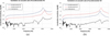 |
Figure 6 Measured acceleration sensitivity of the cylindrical hydrophone and accelerometers with vibrational excitation (a) along the acoustic axis of accelerometer #1 and (b) along the acoustic axis of accelerometer #2. |
4.2 Acoustic test
Figure 7 shows the experimental setup for acoustic testing of the vector sensor. The experiments were performed in a 12 × 18 × 10-m water tank with linear and rotational mobile supports. The vector sensor and three-channel pre-amplifiers were installed in an oil-filled polyurethane tube for waterproof. The vector sensor was compliantly suspended using elastic wire. The vector sensor and reference transducer (ITC 1007) were placed at a depth of 5.5 m, and 4.2 m apart in the water tank. An input sine signal generated from a function generator (Agilent 33522A) is amplified and fed into the reference transducer through a power amplifier (Instruments L20). The measured signals from the accelerometers and the hydrophone are pre-amplified, band-pass filtered (Krohn Hite 3944), and visualized on a digital oscilloscope. The Receiving Voltage Sensitivity (RVS) and directivity patterns of the accelerometers and the hydrophone were measured.
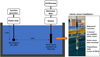 |
Figure 7 The experimental setup for acoustic testing of the vector sensor. |
Figure 8 shows the measured RVS curves of the two accelerometers and hydrophone in the directions of the acoustic axes of (a) accelerometer #1 and (b) accelerometer #2. The accelerometers show the sensitivity proportional to frequency with 6 dB per octave slope below resonance. The RVS of the accelerometer was about −199 dB at 3 kHz. The hydrophone exhibited a flat response over the entire operating frequency range and an RVS of about −196 dB re 1 V/μPa. The responses of accelerometers excited on their acoustic axes were about 25 dB greater than the off-axis responses.
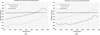 |
Figure 8 Receiving voltage sensitivity of the hydrophone and accelerometers on acoustic excitation (a) along the acoustic axis of accelerometer #1 and (b) along the acoustic axis of accelerometer #2. |
Figure 9 shows the measured and simulated RVS curves of the accelerometers. The simulated curve is calculated from the theoretical model in Chapter 2. The measured RVS curves of the accelerometer #1 and accelerometer #2 are almost identical. The measured and the simulated resonance frequencies are around 4.1 kHz. Both the measured and simulated RVS curves show the 6 dB per octave slope below resonance. However, the measured RVS curve is about 4 dB lower than the measured curves. We suspect that the fabrication condition of the sensor may not be perfect enough. The imperfect adhesion between single crystal plates and base plate or the imperfect base clamping of the cantilever beam may reduce the measured sensitivity.
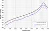 |
Figure 9 Measured and simulated receiving voltage sensitivity of the accelerometers on acoustic axis. |
Figure 10 shows the measured directivity patterns of the two accelerometers and the hydrophone at the frequencies of 1, 2, and 3 kHz. The hydrophone exhibited an omnidirectional directivity pattern over the entire operating frequency. The accelerometers exhibited dipole directivity patterns with figure eight directivity. The directivity patterns of each accelerometer are perpendicular because they are orthogonally mounted. The −3 dB beamwidth of the accelerometer was measured to 90°. The difference between on-axis sensitivity and off-axis sensitivity exceeded 20 dB over the entire operating frequency range.
 |
Figure 10 Measured directivity patterns of the hydrophone and accelerometers at frequencies 1, 2 and 3 kHz. |
4.3 The cardioid beam pattern
Cardioid directivity patterns were generated by summing the signal from the hydrophone and the accelerometers with an inherent phase difference of 90° as shown in equation (15). The phase difference as well as level difference are compensated over the operating frequency range. Figure 11 shows the cardioid directivity patterns formed at frequencies of 1, 2, and 3 kHz. The directivity patterns denoted by the solid and dotted lines are combined cardioid directivity patterns of the hydrophone and the accelerometers. The cardioid beam exhibits a −3 dB beamwidth of about 90°. The difference between the front and back levels exceeds 20 dB. The directional cardioid beam of the vector sensor is verified over the entire operating frequency range.
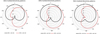 |
Figure 11 Cardioid directivity patterns generated by summing the signal from the hydrophone and the accelerometers at frequencies 1, 2 and 3 kHz. |
5 Conclusion
A vector sensor composed of a cylindrical hydrophone housing containing two orthogonal cantilever beam accelerometers was designed, fabricated, and evaluated in this paper. A theoretical model of a bimorph cantilever beam accelerometer was established to simulate sensitivity of the vector sensor containing various piezoelectric materials. This analysis showed that a cantilever beam accelerometer employing [0 1 1] poled PIN-PMN-PT single crystals has a higher signal-to-noise ratio than accelerometers with other piezoelectric materials. Mounting cantilever beam accelerometers inside a conventional cylindrical hydrophone was proposed for miniaturization of the acoustic vector sensor. The fabricated sensor shows the expected results with a directional cardioid directivity pattern over the operating frequency range. Although the basic functionality of the proposed vector sensor was verified, further study will be carried out to improve sensitivity. The adhesion process of multi-layer structure and the clamping method of the cantilever beam will be investigated. Also, the vector sensor with neutral buoyancy will be investigated by optimizing weight and applying a buoyant material to further increase the sensitivity, since the fabricated sensor had rather heavy weight with negative buoyancy.
Conflict of interest
The authors declare that they do not have any conflict of interest.
Acknowledgments
This work was supported by Ibule Photonics who provides single crystal material and fabrication of the cantilever beam accelerometers.
References
- R.J. Urick: Principles of Underwater Sound. McGraw-Hill, New York, 1983, pp. 54–60. [Google Scholar]
- A.D. Waite: SONAR for Practicing Engineers. Wiley, 1998, pp. 108–109. [Google Scholar]
- P. Santos, P. Felisberto, S.M. Jeusus: Vector sensor arrays in underwater acoustic applications. IFIP Advances in Information and Communication Technology 313 (2010) 316–323. [Google Scholar]
- B.M. Abraham, M.J. Berliner: Directional hydrophones in Towed Systems, in: Proceedings of the Workshop on Directional Acoustic Sensors, Newport, RI, 17–18 April, 2001. [Google Scholar]
- D. Huang: Hybrid Pressure and vector sensor towed array, US 7,599,253 B1, 2009. [Google Scholar]
- A. Thode, J. Skinner, P. Scott, J. Rowsell: Tracking sperm whales with a towed acoustic vector sensor. The Journal of Acoustical Society of America 128, 5 (2010) 2681–2694. [CrossRef] [Google Scholar]
- J. Groen, S.P. Beerens, R. Been, H. Doisy, E. Noutary: Adaptive port-starboard beamforming of triplet sonar array. IEEE Journal of Oceanic Engineering 30, 2 (2005) 348–359. [CrossRef] [Google Scholar]
- S. Simakov, Z.Y. Zhang, R.P. Goddard: Optimal beamforming on synthetic interference and noise for active processing of multiplet line arrays, in: 2015 IEEE Intermational Conference on Acoustics, Speech and Signal Processing (ICASSP) 1 (2015) 2519–2523. [Google Scholar]
- J.M. Crawford, D. Lineas Siurna, C.J. Purcell: Quad Sensor: A new low-frequency active-band directional sensor for towed receiver arrays. Underwater Defense Technology Europe 1 (2008). [Google Scholar]
- J.P. Feuillet, W.S. Allensworth, B. Newhall: Nonambiguous beamforming for a high resolution twin-line array. The Journal of the Acoustical Society of America 97 (1995) 3292–3292. [Google Scholar]
- C.H. Sherman, J.L. Butler: Transducers and arrays for underwater sound. Springer, New York, 2007, pp. 306–324. [Google Scholar]
- T.B. Gabrielson: Design problems and limitations in vector sensors, in: Proceedings of the Workshop on Directional Acoustic Sensors, 2001. [Google Scholar]
- K. Kim, T.B. Gabrielson, G.C. Lauchle: Development of an accelerometer-based underwater acoustic intensity sensor. The Journal of Acoustical Society of America 116, 6 (2004) 3384–3392. [CrossRef] [Google Scholar]
- D.A. DeAngelis, G.W. Schulze: Performance of PIN-PMN-PT single crystal piezoelectric versus PZT8 piezoceramic materials in ultrasonic transducers. Physics Procedia 63 (2015) 21–27. [Google Scholar]
- L.M. Ewart, E.A. McLaughlin, H.C. Robinson, J.J. Stace, A. Amin: Mechanical and electromechanical properties of PMNT single crystals for naval sonar transducers. IEEE Transactions on Ultrasonics, Ferroelectrics, and Frequency Control 54, 12 (2007) 2469–2473. [CrossRef] [PubMed] [Google Scholar]
- J.A. Brown, K. Dunphy, J.R. Leadbetter, R.B.A. Adamson, O. Beslin: Fabrication and performance of a single-crystal lead magnesium niobate-lead titanate cylindrical hydrophone. The Journal of Acoustical Society of America 134, 2 (2013) 1031–1038. [CrossRef] [Google Scholar]
- B.P. Raaja, R.J. Daniel: A simple analytical model for MEMS cantilever beam piezoelectric accelerometer and high sensitivity design for SHM (structural health monitoring) applications. Transactions on Electrical and Electronic Materials 18, 2 (2017) 78–88. [CrossRef] [Google Scholar]
- C.R. Browen, H.A. Kim, P.M. Weaver, S. Dunn: Piezoelectric and ferroelectric materials and structures for energy harvesting applications. Energy and Environmental Science 7 (2014) 25–44. [CrossRef] [Google Scholar]
- L. Zhang, K.A. Williams, Z.C. Xie: Evaluation of analytical and finite element modeling on piezoelectric cantilever bimorph energy harvester. Transactions of the Canadian Society for Mechanical Engineering 37, 3 (2013) 624–625. [CrossRef] [Google Scholar]
- H. Zhang, H.-J. Chen, W.-Z. Wang: An underwater acoustic vector sensor with high sensitivity and broad band. Sensors & Transducers 170, 5 (2014) 30–34. [Google Scholar]
Cite this article as: Cho Y, Je Y & Jeong WB. 2020. A miniaturized acoustic vector sensor with PIN-PMN-PT single crystal cantilever beam accelerometers. Acta Acustica, 4, 17.
All Tables
Figure of merit for vector sensors containing piezoelectric materials: [0 1 1] poled PIN-PMN-PT, [0 0 1] poled PIN-PMN-PT, PZT 5H, and PZT4.
All Figures
|
Figure 1 (a) Bimorph cantilever beam accelerometer under base excitation, and (b) Vector sensor with cantilever beam accelerometers and a cylindrical housing. |
| In the text | |
|
Figure 2 (a) Pressure sensitivity and (b) signal-to-noise ratio of a cantilever beam vector sensor containing various piezoelectric materials: [011] poled PIN-PMN-PT, [0 0 1] poled PIN-PMN-PT, PZT 5H, and PZT4. |
| In the text | |
|
Figure 3 The vector sensor design: (a) Bimorph cantilever beam accelerometer clamped by an endcap, and (b) vector sensor with cylindrical hydrophone and cantilever beam accelerometers mounted inside the hydrophone. |
| In the text | |
|
Figure 4 Fabrication process of the vector sensor. |
| In the text | |
|
Figure 5 Experimental setup for vibration testing of the vector sensor. |
| In the text | |
|
Figure 6 Measured acceleration sensitivity of the cylindrical hydrophone and accelerometers with vibrational excitation (a) along the acoustic axis of accelerometer #1 and (b) along the acoustic axis of accelerometer #2. |
| In the text | |
|
Figure 7 The experimental setup for acoustic testing of the vector sensor. |
| In the text | |
|
Figure 8 Receiving voltage sensitivity of the hydrophone and accelerometers on acoustic excitation (a) along the acoustic axis of accelerometer #1 and (b) along the acoustic axis of accelerometer #2. |
| In the text | |
|
Figure 9 Measured and simulated receiving voltage sensitivity of the accelerometers on acoustic axis. |
| In the text | |
|
Figure 10 Measured directivity patterns of the hydrophone and accelerometers at frequencies 1, 2 and 3 kHz. |
| In the text | |
|
Figure 11 Cardioid directivity patterns generated by summing the signal from the hydrophone and the accelerometers at frequencies 1, 2 and 3 kHz. |
| In the text | |
Current usage metrics show cumulative count of Article Views (full-text article views including HTML views, PDF and ePub downloads, according to the available data) and Abstracts Views on Vision4Press platform.
Data correspond to usage on the plateform after 2015. The current usage metrics is available 48-96 hours after online publication and is updated daily on week days.
Initial download of the metrics may take a while.