| Issue |
Acta Acust.
Volume 4, Number 5, 2020
|
|
|---|---|---|
| Article Number | 18 | |
| Number of page(s) | 11 | |
| Section | Musical Acoustics | |
| DOI | https://doi.org/10.1051/aacus/2020018 | |
| Published online | 29 October 2020 | |
Scientific Article
The link between the tonehole lattice cutoff frequency and clarinet sound radiation: a quantitative study
LMA, CNRS, UPR 7051, Aix-Marseille Univ, Centrale Marseille, 13453 Marseille Cedex 13, France
* Corresponding author: This email address is being protected from spambots. You need JavaScript enabled to view it.
Received:
7
April
2020
Accepted:
31
August
2020
Abstract
Musical instruments are said to have a personality, which we notice in the sound that they produce. The oscillation mechanism inside woodwinds is commonly studied, but the transmission from internal waveforms to radiated sound is often overlooked, although it is musically essential. It is influenced by the geometry of their resonators which are acoustical waveguides with frequency dependent behavior due in part to the lattice of open toneholes. For this acoustically periodic medium, wave propagation theory predicts that waves are evanescent in low frequency and propagate into the lattice above the cutoff frequency. These phenomena are generally assumed to impact the external sound perceived by the instrumentalist and the audience, however, a quantitative link has never been demonstrated. Here we show that the lattice shapes the radiated sound by inducing a reinforced frequency band in the envelope of the spectrum near the cutoff of the lattice. This is a direct result of the size and spacing between toneholes, independent of the generating sound source and musician, which we show using external measurements and simulations in playing conditions. As with the clarinet, the amplitude of the even harmonics increases with frequency until they match odd harmonics at the reinforced spectrum region.
Key words: Clarinet / Cutoff frequency / Tonehole lattice / Radiation / Woodwind
© E. A. Petersen et al., Published by EDP Sciences, 2020
 This is an Open Access article distributed under the terms of the Creative Commons Attribution License (https://creativecommons.org/licenses/by/4.0), which permits unrestricted use, distribution, and reproduction in any medium, provided the original work is properly cited.
1 Introduction
Woodwind instruments are complex objects with geometries that have evolved through empirical experimentation over centuries. The resonator bore can be predominantly cylindrical or conical, and many instruments terminate in a bell that has yet another cross section profile. The position and size of the toneholes are chosen to balance intonation and timbre, and each hole affects the influence of the others. While these geometrical variations are often subtle, they may have a strong influence on the sound of an instrument.
The playing frequency of a woodwind instrument is largely determined by the distance between the reed and the first open tonehole, and to a first approximation the downstream toneholes are ignored. However, in many instruments this “unused” lattice of toneholes acts as an acoustic high pass filter, thereby modifying the response of the resonator and, eventually, the radiated sound [1]. The low frequency first hole approximation and the high frequency lattice filtering are separated by the tonehole lattice cutoff frequency f c, and is due to the pass and stop bands of waves propagation in periodic media [2]. The existence of a cutoff frequency is a communality among many different woodwinds including the clarinet, saxophone, bassoon, and tárogató [1]. Some instruments, such as the Kaval [3], even have additional toneholes that are never closed during normal playing, which may have been introduced to serve as a lattice for the lowest notes of the instrument.
The cutoff frequency is generally assumed to influence the sound that an instrument makes, possibly even mapping to certain adjectives used by musicians to describe the “character” of a given instrument. However, there are few quantitative links between the cutoff and radiated sound [4, 5]. In his final article [6], Benade and Lutgen published a study connecting room-averaged external spectra across the first register of the saxophone, demonstrating a frequency band with increased radiation centered at what he calls the “break frequency.” For the saxophone, he asserts that the break frequency in the spectra of the radiated sound is related to the tonehole lattice cutoff. This interpretation is complicated, however, because there is no rigorous definition of the cutoff frequency of a real instrument. Furthermore, a recent article demonstrates that, in contrast to the clarinet, the cutoff frequency of the saxophone varies considerably over the range of the first register [7].
Attempts to study the tonehole lattice cutoff of real instruments generally fall either into empirical or analytic methods, both of which have flaws. One empirical approach is to define the cutoff frequency from an input impedance measurement by identifying a perturbation in the modulus or argument of the input impedance or reflection coefficient. This is often done by human judgment, although it is also possible to apply arbitrary thresholds, and both methods have merits and drawbacks. Analytic approaches can be adapted from the theory of wave propagation in periodic media [8], although the finite and lossy nature of the resonators complicates the analogy. Furthermore, the lattices of real instruments are not typically periodic, so it is necessary to extend the theory in one of several ways by considering, for example, pairs of adjacent toneholes [9]. One form of analysis may be more appropriate than another for a specific family of instruments. An instrument with a high degree of acoustical regularity, such as the clarinet [10], seems more suitable for the analytic approach than an instrument that is highly irregular, such as the bassoon. Furthermore, some instruments have cutoffs that evolve in conjunction with the changing notes of a chromatic scale, such as the saxophone. In this case an empirical approach may be more appropriate because the lattice is less periodic (geometrically and acoustically) than a clarinet.
In order to avoid the inherent ambiguity surrounding the cutoff frequency of real instruments, the current work starts with simplified resonators that have been analytically designed with constant chosen cutoffs. This has the advantage that external spectral characteristics are expected to be directly linked to the cutoff frequency of the resonators. However, because the cutoffs of the resonators used in these experiments are strong and unambiguous, care must be taken when extrapolating to real instruments, which may have ambiguous or diffuse cutoffs as well as other competing behavior due to the conicity, the bell, and additional geometric differences. Because it is difficult to design and impractical to construct conical resonators with strong cutoffs, the simplified resonators used in this study are cylindrical, and the results are mainly applicable to instruments in the clarinet family.
The basic theory of tonehole lattice cutoff frequencies is reviewed in Section 2, and applied towards the design of simplified resonators with known cutoffs. Experimental results of external sound field measurements using the simplified resonators are discussed in Section 3, with complementary simulations in Section 4. Application to a clarinet recorded in anechoic conditions is treated in Section 5, followed by concluding remarks in Section 6.
2 Basic theory
2.1 The tonehole lattice cutoff frequency
The cutoff frequency is determined by the geometry of a constituent cell of the lattice, depending on the radius of the main bore, the tonehole radius, chimney height, and inter-hole spacing, shown in Figure 1. The geometry of a lattice can be designed to have a desired cutoff frequency [10–12]. While a true cutoff exists only for infinite, lossless lattices [2], a strong cutoff behavior can exist for finite resonators with at least two or three open toneholes. Furthermore, the theory is developed for geometrically regular lattices consisting of repeating, identical cells, which is in contrast with the geometric irregularity of real instruments. However, it has been shown that an acoustic regularity may be achieved even for geometrically irregular lattices with no adverse impact of the cutoff of the lattice, which reinforces the application of cutoff theory to real instruments.1 It is convenient, though not necessary, to design the acoustically regular lattice to also be geometrically regular. In this case, the cutoff frequency of the lattice is achieved if the constituent cell is designed according to
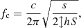 (1)where c is the speed of sound in air, s = πb
2 is the cross section of the tonehole, S = πa
2 that of the main bore, h the height of the hole, and
(1)where c is the speed of sound in air, s = πb
2 is the cross section of the tonehole, S = πa
2 that of the main bore, h the height of the hole, and  the distance between two subsequent holes. Equation (1) corresponds to the eigenfrequency of the cell assuming rigid conditions at the extremities of the main bore [11]. Variations of this formula can be derived for more complicated geometries, including conical resonators [7].
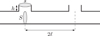 |
Figure 1 Geometrical dimensions of a tonehole pair. When repeated, this element forms a regular lattice with a cutoff frequency provided by equation (1). |
For the purposes of this study, a lattice with at least five open toneholes designed following equation (1) is considered to have a tonehole lattice cutoff, even though the theory is derived under the assumption of an infinite, lossless lattice. The resonators presented in Section 2.2 and analyzed in Sections 3 and 4 follow this definition and are said to have a strong cutoff, which can be clearly identified to reasonable precision on measurable characteristics such as the input impedance or reflection coefficient. Real instruments, however, do not generally respect equation (1), and may only exhibit a weak or diffuse cutoff whose precise determination is not obvious from measurement or theory, but still recognizable as an effect of the lattice.
2.2 Resonators designed to have cutoffs at chosen frequencies
Four resonators are designed and produced for this study. The resonators are built using stiff, cylindrical plastic tubing, three of which are pierced with toneholes, resembling the geometry of a clarinet. The fourth resonator is a simple cylinder without toneholes. A clarinet mouthpiece can be inserted at the upstream end of the resonators. As for a real instrument, the portion of the duct upstream from the lattice determines the playing frequency of the highest note, and the lattice toneholes can be consecutively closed to achieve lower notes. In contrast with a real clarinet, the size and location of the toneholes are not designed to produce the notes of a specific musical scale, but rather to present an acoustically periodic lattice that alters the high frequency response of the resonator.
All four resonators are designed to have the first impedance peak at approximately 185 Hz when all toneholes are open, and the three resonators with tonehole lattices have cutoffs at 1.0, 1.5, and 2.0 kHz [12]. Each resonator, except the simple cylinder, has 10 toneholes. The input impedance and geometries of the resonators are shown in Figure 2 and Table 1, respectively. The cutoff is evident for the three resonators with lattices, seen as a change in spacing and height of the impedance peaks. The regularly spaced peaks characteristic of a quarter wavelength resonator are seen for the simple cylinder.
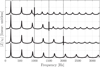 |
Figure 2 Simulated input impedance modulus for (top to bottom) resonators with f c = 1.0, 1.5, 2.0 kHz, and a cylinder with no tonehole lattice, vertical offset for clarity. Normalized by characteristic impedance z c of the duct. |
Geometrical dimensions of three resonators with the same first impedance peak f
1 and different cutoff frequencies f
c. First peak and cutoff frequencies in Hz, all other quantities in mm. The first hole is located at  . Consider
  for the cylinder.
In order to maintain a strong cutoff for different fingerings, at least five consecutive, downstream toneholes remain open for all measurements. This results in six possible notes per resonator with fundamentals ranging from 114 Hz to 154 Hz under playing conditions. Because the lattices are acoustically regular, each of these six notes has a nearly identical cutoff.
2.3 Radiation characteristics above and below the tonehole lattice cutoff frequency
The radiation of a resonator with a tonehole lattice has significant differences for frequencies below and above the cutoff. Below the cutoff, the wave does not propagate into the lattice, so the resonator predominantly radiates as a monopole source from the first open tonehole. Above the cutoff, the wave does propagate into the lattice and radiates from subsequent toneholes and the termination of the resonator. The wave also reflects back into the resonator from the termination of the lattice [11, 13]. Above the cutoff, the contributions from multiple radiating apertures create complicated radiation properties, which can affect the directivity and efficiency of the resonator.
At the cutoff, the phase speed within the resonator is very high and the flow through the toneholes is nearly in phase, creating a strong directivity lobe perpendicular to the lattice. Above the cutoff, the flow through the toneholes is no longer in phase and the radiation is characterized by complicated directivity lobes. Frequencies well above cutoff propagate in the lattice and only weakly radiate from the toneholes, mainly reflecting and radiating from the termination of the resonator. For the simplified resonators, the cutoff frequency is at a rapid transition between these two frequency band behaviors, while the distinction is more complicated for real instruments for which the inter-hole spacing is not uniform and the different tonehole radii influence the radiation efficiency of each source.
3 External sound field measurements of simplified resonators
3.1 Basis for measurement protocol
The methodology follows the protocol developed by Benade to measure the radiated sound fields of woodwind instruments, notably for the clarinet and saxophone [6, 14]. In contrast with most acoustical measurement requirements, Benade realized that it is informative to measure the spectral radiation characteristics of instruments in musically appropriate environments. The defining sound features of an instrument family are easily identified by experienced listeners regardless of the room in which they are played. Benade concludes that the spectral characteristics that are relevant to human perception could also be measured in “normal” rooms, i.e. not under anechoic conditions, and that the results describe the instrument under the same conditions for which an audience typically consumes music. To avoid complications due to the strong directivity of many instruments, the instrument and microphone should be placed far apart, and both should be slowly moving to introduce a type of “room averaging.” The protocol and its implications are detailed in several documents [15, 16].
3.2 Details of measurements
The simplified resonators are outfitted with a clarinet mouthpiece and a Plasticover (RICO-RP05BCL200) strength 2 B♭ clarinet reed in order to be played by a musician. The room is a medium sized lecture hall with 122 seats on a steep incline and an approximate volume of 730 m3. This room is chosen because it has light acoustic treatment and is a reasonable example of a musically appropriate environment. This is desirable because the purpose of the study is to identify global spectral characteristics of the resonators in realistic playing conditions.
Each of the six notes with fundamentals ranging from 114 to 154 is played for approximately 20 s for both forte and piano dynamics, subjectively determined by the musician. In order to avoid inconsistencies due to strong directivity lobes of the resonator, the musician slowly sways the instrument back and forth with a period of about 4 s. Four microphones are used to record the signal in the room: a DPA-4099 instrument microphone attached to the resonator approximately 8 cm above the center of the lattice, two stationary Neumann KM 184 (cardioid) microphones at a distance 8 m and 12 m from the musician, and a Neumann U87 (cardioid operating mode) at a distance of approximately 4 m. The U87 is manually waved back and forth with an approximate period of 4 s to provide some spatial averaging in the room. Therefore, there are 152 distinct signals: 3 resonators with 6 notes each, plus the simple cylinder, each with two dynamics, measured by four microphones. The data from the DPA is not used in the analysis because, due to its position just above the lattice and in a directivity lobe at cutoff, its data suggest a greater effect than what is measured by the more distant microphones.
Preliminary results are shown as spectrograms in Figure 3. Resonators with f c = 1.0, 1.5, and 2.0 kHz are displayed from left to right, with forte playing levels on top and piano playing levels on bottom. The measurements from the Neumann U87 and two Neumann KM 184 are combined into a composite signal. The steady state portions of each note are extracted from each microphone channel, highpass filtered at 100 Hz by the MATLAB highpass function, which uses a minimum-order filter with a Kaiser window resulting in a 60 dB stop band attenuation. The signals are then normalized by their root-mean-square value. These signals are available online as Supplementary Material. The power spectral density is calculated for successive Hann-windowed segments of 213 samples using a 50% overlap. The resulting spectra from the three microphones are summed, normalized by the maximum value at each time step, and plotted in decibel representation.
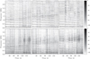 |
Figure 3 Spectrograms of six notes played in a descending scale using a clarinet mouthpiece. Top panels at forte and bottom panels at piano playing levels for resonators with, from left to right, f c = 1.0, 1.5, 2.0 kHz. The analysis is performed on composite signals from the Neumann U87 and two Neumann KM 184. Color map in decibels. |
These spectrograms demonstrate room averaged characteristics of the sound field radiated by individual notes of each resonator. The average spectral centroid for the resonators with f c = 1.0, 1.5, and 2.0 kHz cutoffs is 0.55, 0.94, 1.12 kHz at forte playing levels, and 0.28, 0.22, 0.27 kHz at piano playing levels. This may be due to the appearance of additional energy around the cutoff of each resonator. This possible reinforced frequency region, particularly in this representation, may be partially hidden by the imparity between even and odd harmonics characteristic to cylindrical resonators. Nonetheless, these spectrograms are suggestive of an influence of the cutoff on radiation, although additional processing is needed to determine a quantitative link.
The data presented in Section 3.4 correspond to these three resonators. However, in deference to the measurement protocol proposed by Benade, only the Neumann U87 data is included in the following analysis.
3.3 Data processing
The same signal treatment is used for three different experiments in this study: in situ measurements of simplified resonators described in Section 3.2, the simulated replication of these measurements in Section 4, and anechoic recordings of a real clarinet in Section 5. Some preliminary steps are necessary for the simulations and anechoic recordings to reduce multiple channels of data into a single channel. These additional procedures are outlined in Sections 4.3 and 5. Once reduced, all the data are processed as follows.
The data of a given resonator consists of separate audio files, one for each note that is considered in the analysis. For each note, the signal is truncated to include only the steady-state portion of the tone to discard attack and decay transients. Furthermore, each signal has considerable variation in sound pressure level and timbre due to the directivity of the resonator, movement of the player, movement of the measurement microphone, and fluctuating control parameters. Therefore, the signal is analyzed in 0.5 s segments and treated with a Hann window of the same duration. The spectra is generated using the built-in MATLAB FFT, and handled to be proportional to units [Pa2/Hz]. The harmonics in the spectra are then extracted using a peak detection scheme. Because the quantity of interest is the spectral envelope, an exact calibration is not necessary and results are depicted in normalized representations. This procedure is repeated for the remaining notes for the resonator.
The basic data set for each resonator is now the harmonic frequency and amplitude pairs at 0.5 s intervals for multiple fingerings. To demonstrate the global radiation characteristics of the resonator it is helpful to average the data. Several different approaches are used and described in the corresponding sections.
3.3.1 Measurement averaging
The signal from the Neumann U87 microphone used in Figure 4 is first treated following the protocol described in Section 3.3. This results in approximately 240 “instances” of the spectrum per resonator, calculated from six fingerings, each with 20 s of data divided into time frames of 0.5 s. In order to visualize the data, the statistical variation of each harmonic is depicted using box plots. Each box corresponds to the n th rank harmonic from all the fingerings, excluding outliers. For example, the left-most black box in each panel depicts the amplitude variation of the fundamental for all six fingerings, while the left-most red box depicts the first even harmonics of all six fingerings. The boxes are positioned at the average frequency of the n th rank harmonic of the six fingerings. The lower and upper limits of the boxes mark the 25th and 75th percentiles. The median value of the odd and even harmonics are traced in black and red, respectively. Because this plot represents data with a large variation in amplitude, the upper contour of the whiskers tend to match a naive inspection of the raw data.
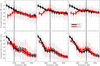 |
Figure 4 Measured external spectra, averaged over six notes played on each of three resonators with different cutoff frequencies. Top panels depict forte dynamics and bottom panels depict piano dynamics. Each box plot is computed from the n th rank harmonic to present an averaged spectra that is characteristic to the resonator across different fingerings with fundamentals ranging from 114 Hz to 154 Hz, and is positioned at the average frequency of the respective n th rank harmonic. Data from manually waved microphone (Neumann U87 4 m distance). Black: odd harmonics, red: even harmonics, vertical line: cutoff frequency of the resonator. Box plots within hatched area have atleast one harmonic near cutoff. Solid black and red lines trace the median of each box plot. The median amplitude of the fundamentals are normalized to 0 dB in each panel. Boxes span from 25th to 75th percentiles and thin lines show the span of the data ignoring outliers. |
3.4 The reinforced spectrum region of the radiated sound field
The external spectra for all three resonator cutoff frequencies for both forte (top) and piano (bottom) dynamics are depicted in Figure 4. Below the cutoff of each resonator, the even harmonics are several decades weaker than the odd harmonics, as is expected of a quarter wave resonator. However, for the forte playing dynamic, the envelope of the even harmonics increases with frequency towards a maximum value near the cutoff of the resonator, above which the even and odd harmonics are equally strong. Although it is less obvious in this representation of the data, odd harmonics are also reinforced, seen here mainly by the envelope of the box plot whiskers. Figure 5, which uses the averaging scheme described in Section 4.4, shows more clearly that the reinforced spectrum region consists of both even and odd harmonics.
 |
Figure 5 Comparison between measured (solid) and simulated (dashed) external spectra in a decibel representation for three resonators with cutoffs f c = 1.0, 1.5, 2.0 kHz at forte playing conditions. Odd harmonics are depicted in black and even harmonics in red. Synthesis control parameters provided in Section 4.2. |
The lower panels of Figure 4 show that the effect of the cutoff is not as pronounced for piano playing dynamics, although the cutoff of the resonator does influence the shape of the spectral envelope. The slope of the envelope is much steeper than for the forte data because a softly played note is generally not as harmonically rich as one that is played loudly, and most of the energy is contained in the first several harmonics. Therefore, the reinforced spectrum region is weaker because it falls in a frequency range that does not have a lot of power in the internal waveform.
Repeating the same measurements with a simple cylinder (not depicted for brevity) demonstrates that the reed resonance f r (see Sect. 4.2) may be a competing mechanism that can influence the spectral envelope. In particular, there is a convergence of even and odd harmonics at approximately 1.5 kHz, despite no tonehole lattice. Additional simulations suggest that this convergence is due to the reed resonance. This could be developed as a simple experimental method for coarsely estimating the resonance of a reed. For real clarinets, the cutoff and reed resonance occur at approximately the same frequency f c ≈ f r ≈ 1.5 kHz [17]. It is unclear how these parameters evolved towards the same value, and to what degree this is intentional. A future project could address how each parameter impacts the playability of an instrument.
4 External sound field simulations of simplified resonators
The external sound field of simplified resonators played with a clarinet mouthpiece measured in Section 3 is simulated by combining digital synthesis and a simplified radiation model. The external sound field simulations are implemented in two main stages. The first computes the characteristics of the passive, linear resonators, yielding the input impedance and transfer functions between the input of the resonator and each tonehole. The input impedance is then used with a digital synthesis code to simulate the pressure and flow waveforms inside the mouthpiece. The transfer functions calculated in the first stage translate the flow waveform inside the mouthpiece to the corresponding flow through each tonehole, which radiate into the surrounding space.
4.1 From TMMI to external sound field simulations of passive resonator
The resonators are modeled as passive, linear waveguides that can be characterized independent of the source signal. As a first approximation, nonlinear effects due to high internal sound pressure levels as well as nonlinear effects in the toneholes are ignored. Although the simulation model ignores the nonlinear effects in the toneholes, the qualitative agreement between simulation and experiment is satisfactory. While accounting for these nonlinear aspects would likely improve the simulations, particularly at forte playing levels, it is outside the scope of this article to develop the nonlinear tonehole model, which is an open research topic.
First, the input impedance of the resonators is simulated using the Transfer Matrix with External Interactions (TMMI) [18], which is related to the transfer matrix method but accounts for external interactions of toneholes that radiate into the same space. Accounting for mutual radiation impedance improves the simulation of the input impedance, particularly above the cutoff.
In order to simulate the radiated sound field, the TMMI algorithm has been modified to compute the frequency domain pressure P n (ω) and flow U n (ω) at the n th aperture (tonehole and termination of the resonator) resulting from an arbitrary source pressure P s (ω) or flow U s (ω) at the input. Therefore, the passive response of the resonator can be described by a set of transfer functions between the input of the resonator and all radiating apertures:
 (2)
(2)
The far field external pressure at an observation point O is the superposition of the contribution of each source term U n (ω)
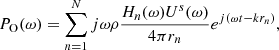 (3)where r
n
is the distance between O and the n
th source, ω is the angular frequency, k the wave number, c and ρ the speed of sound and density of air. Each source term is treated as a monopole and diffraction due to the resonator is ignored. This development can be used to simulate the radiation properties of the resonators regardless of the driving source.
(3)where r
n
is the distance between O and the n
th source, ω is the angular frequency, k the wave number, c and ρ the speed of sound and density of air. Each source term is treated as a monopole and diffraction due to the resonator is ignored. This development can be used to simulate the radiation properties of the resonators regardless of the driving source.
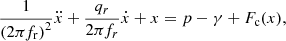
4.2 Digital sound synthesis
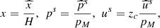
Digital synthesis is used to simulate the pressure and flow inside the mouthpiece in the discrete time domain. In this simulation, the action of the musician is represented by two dimensionless control parameters [19], defined by
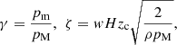 (4)where p
m is the pressure inside the mouth of the musician, p
M is the reference pressure necessary to close the reed channel completely, w and H are the width and height of the reed channel at rest, and z
c is the characteristic impedance of the resonator. The variables of the model discussed in this work are the reed displacement x and the acoustic pressure p
s and flow u
s
at the input of the resonator, given in dimensionless form by
(4)where p
m is the pressure inside the mouth of the musician, p
M is the reference pressure necessary to close the reed channel completely, w and H are the width and height of the reed channel at rest, and z
c is the characteristic impedance of the resonator. The variables of the model discussed in this work are the reed displacement x and the acoustic pressure p
s and flow u
s
at the input of the resonator, given in dimensionless form by
 (5)where the hat notation signals the variable’s physical value. The time-domain synthesis scheme follows previous work [20].
In order to accurately represent the high frequency behavior of the resonator, a reflection function formalism [21] is preferred over a truncated modal representation. The reflection function r links the reflected wave  to the outgoing wave
  through the relation
 (6)where * denotes the convolution product. Note that r is deduced from the input impedance as the inverse Fourier transform of the reflection coefficient. In the discrete form, it is truncated to the first 0.1 s, long enough to accurately represent low frequencies which have the longest response due to weak losses.
The reed is modeled by a damped single degree-of-freedom oscillator. Its dimensionless displacement from equilibrium follows the form
 (7)where f
r is the reed eigenfrequency and q
r its damping coefficient. The force F
c, accounting for the contact with the mouthpiece lay [22], is defined by
(7)where f
r is the reed eigenfrequency and q
r its damping coefficient. The force F
c, accounting for the contact with the mouthpiece lay [22], is defined by
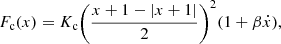 (8)with nonlinear stiffness K
c and a damping coefficient β. The nonlinear characteristic derived from Bernoulli’s law that determines the flow through the reed channel is
(8)with nonlinear stiffness K
c and a damping coefficient β. The nonlinear characteristic derived from Bernoulli’s law that determines the flow through the reed channel is
 (9)
(9)
The nonsmooth functions in equations (8) and (9) are regularized: the absolute values |·| are replaced by  [23]. The value of the parameters used to obtain the simulation are summarized in Table 2.
Digital sound synthesis parameters pertaining to reed dynamics. All unitless except f r, in Hz.
The control parameters, corresponding to pressure inside the mouth γ and musicians lips ζ, are slowly varied to approximate a real musician. A simultaneous variation of γ and ζ over a T = 10 s signal follows the form
 (10)
(10)
 (11)where γ
c, γ
a, ζ
c, and ζ
a are constants, summarized in Table 3 for forte and piano playing levels [24, 25]. The static portion of the control parameters are chosen to create beating conditions for the forte playing level and to be near the threshold of oscillation for the piano playing level [26, 27]. The control parameters are varied slightly around static values using trigonometric functions because they are smooth, real valued, periodic, and well-known. This is intended to mimic the measurement conditions for which there was some variation in musician control due to the slow movement required by the measurement protocol.
(11)where γ
c, γ
a, ζ
c, and ζ
a are constants, summarized in Table 3 for forte and piano playing levels [24, 25]. The static portion of the control parameters are chosen to create beating conditions for the forte playing level and to be near the threshold of oscillation for the piano playing level [26, 27]. The control parameters are varied slightly around static values using trigonometric functions because they are smooth, real valued, periodic, and well-known. This is intended to mimic the measurement conditions for which there was some variation in musician control due to the slow movement required by the measurement protocol.
4.3 Combining digital synthesis and radiation models
The external sound field of the instrument under playing conditions is simulated through the linear transformations of the waveforms inside the mouthpiece computed by digital synthesis. The acoustic flow  in the mouthpiece produced by digital synthesis is transformed to the frequency domain
  , and the resulting flow through each tonehole is calculated using
  . The pressure
  at an observation point O is calculated as the inverse Fourier transform of P
O(ω), provided by equation (3).
at an observation point O is calculated as the inverse Fourier transform of P
O(ω), provided by equation (3).
Because each source term is treated as a monopole, the resonator is considered to radiate symmetrically about its axis. Therefore, the external sound field is simulated in two dimensions, with observation points O laying on a plane that includes the axis of the resonator. The first open tonehole defines the origin and 100 equally spaced observation points are defined along a circle with a 10 m radius centered at the origin.
This configuration is treated as an approximation of the sound power of the source in an anechoic environment. The waveforms P O as simulated at each position O are summed directly to produce a single composite waveform, which is processed as described in Section 3.3. This approximates the spatial averaging of the measurements, and helps avoid inadvertently favoring or neglecting frequency ranges that correspond to strong directivity lobes of the resonator.
4.4 Comparison between measurements and simulation
The simulation results for the three simplified resonators are presented in Figure 5, which also includes the measurements from Section 3. The simulated results use the synthesis parameters in Table 2 and musician control parameters corresponding to a forte dynamic in Table 3. The odd and even harmonics have been averaged using MATLAB function movmean with a five point window, and then smoothed. This averaging allows considerable structure of the spectrum to remain in the plots while suppressing the clutter of raw data points or box plots, making it easier to compare the four overlaying curves.
The most successful feature of the simulated curves is the increase in amplitude of the even harmonics as they approach the cutoff. The reinforced spectrum region is not evident in the simulated odd harmonics, although this could be due to the choice of control parameters. The odd and even harmonic parity above 3.0 kHz (and continuing off the graph), is accurately simulated, although the total energy at high frequencies is underpredicted compared to the measurements. This could be due to the model of mutual radiation impedance between neighboring holes, which is known to influence the total radiation of an acoustic source.
The simulations for the piano playing dynamic (not shown) do not correspond to the measurements as well, although this could be due to inaccurate choice of musician control parameters. However, the scope of this article is to investigate the effect of the cutoff frequency on radiated sound, which has a greater effect at forte playing levels. Therefore, the threshold for appropriate control parameters for a piano dynamic is not pursued.
5 Radiated spectra of a clarinet
To contextualize the academic results of Sections 3 and 4, a similar analysis is applied to a Herbert Wurlitzer Solistenmodell B♭ clarinet using measurements from a publicly available data base [28]. The data used in the current study consists of a 32 channel microphone array in an anechoic environment, with each note of the instrument held for approximately 3 s at a forte playing dynamic. As with the simulations in Section 4, the total radiation of the instrument of a given note is approximated by the sum of signals from different measurement locations, in this case 32 channels in a sphere around the clarinet. This composite signal of each note is processed following the procedure described in Section 3.3.
The results for portions of three registers of the clarinet are shown in Figure 6. The lowest notes of each register are neglected to ensure at least two open toneholes in the lattice. The notes included in the analysis are, from panels top to bottom, E3–E4 (165–330 Hz), B4-A♯5 (494–932 Hz), and D6-A♯6 (1175–1865 Hz).
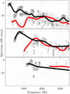 |
Figure 6 Radiated spectra of a real clarinet measured in anechoic conditions played at a forte level. Portions of the first (E3–E4), second (B4-A♯5), and third (D6-A♯6) registers are plotted from top to bottom. Raw data depicted by dark grey and light grey circles, plus their moving average by black and red lines, for odd and even harmonics, respectively. Data accessed through a publicly available data base [28]. |
Qualitatively, the trends pertaining to the simplified resonators are also present for the real clarinet for the first and second registers. The even harmonics increase towards a local maximum between 1.0 and 2.0 kHz, the nominal cutoff frequency of a clarinet. This appears more clearly in the second register, possibly because the reinforced spectrum region is produced by low ranking harmonics. The cutoff frequency is approximately the same for the first two registers because the sound is filtered by essentially the same lattice. For the third register, the notes have fundamental frequencies that are near the cutoff frequency of the lattice, so there is no consistent evolution towards a reinforced spectrum region at the cutoff frequency.
Although the results of the clarinet are generally similar to the simplified resonators, it is not appropriate to make a direct comparison because a clarinet is not an acoustically (or geometrically) regular resonator, so an exact lattice cutoff frequency does not exist. For example, unlike the simplified resonators, the even harmonics of the first register continue to increase after the nominal cutoff, to a maximum at approximately 2.3 kHz. This may be due to the bell of the clarinet, which has a resonance at 2.1 kHz and is not included on the simplified resonators.
The results from the real clarinet shown in Figure 6 are consistent with those reported by Benade and Kouzoupis (Figs. 6–10) [14]. The coherence between these results demonstrates the robustness of his measurement protocol, which is considerably easier to implement compared with a multiple channel anechoic measurement. Furthermore, the reinforced spectrum region in the radiated sound field of the clarinet for both in situ and anechoic measurements provides justification for the anechoic simulation conditions in Section 4.
6 Conclusion
Simplified clarinet-like cylindrical resonators radiate with a reinforced spectrum region that appears near the cutoff frequency of the tonehole lattice. The reinforced spectrum emerges as the even harmonics grow in amplitude to become equally strong as the odd harmonics at the cutoff. This effect on the external sound field is a result of the geometry of the lattice, and provides a direct link between the tonehole lattice and spectral characteristics of the radiated sound. The phenomenon is more pronounced at loud playing dynamics, but also affects the spectral envelope for soft dynamics. Digital synthesis coupled with a radiation model is sufficient to reproduce the measurement results through simulation. Results from a real clarinet, recorded in playing conditions in an anechoic chamber, demonstrate that a reinforced spectrum region also exists near the nominal cutoff of a real clarinet.
A similar evolution of even harmonics in the external sound field was demonstrated by Benade for the clarinet, along with the related break frequency for the saxophone. However, because the saxophone is an acoustically irregular lattice, the link between the tonehole lattice cutoff frequency and the region of reinforced spectrum is not conclusive. Furthermore, because the saxophone is conical, the reinforced spectrum appears as the odd and even harmonics both increase towards the approximate cutoff, in contrast with the current study of cylindrical resonators, for which the increase is primarily observed for the even harmonics. The effects of conical instruments on reinforced spectrum has also been studied for another conical instrument, the bassoon [29].
As suggested by Benade, the tonehole lattice cutoff frequency is generally assumed to influence the character of a woodwind instrument. This study provides one quantitative link between the cutoff and external spectral characteristics that are measurable in musically appropriate environments. While a musician can manipulate the timbre of a note by adjusting the blowing pressure and lip contact with the reed, the reinforced spectrum at cutoff is a consequence of the resonator’s geometry, which is decided by the manufacturer. This allows the possibility of using the cutoff as a design parameter for new instruments. Future work could involve mapping the cutoff to perceptual descriptions of timbre.
Conflict of interest
The authors declare that they do not have any conflict of interest.
Supplementary materials
Two audio files from the in situ recordings are provided to demonstrate the perceptual differences between the three academic resonators. Both files are from the U87 microphone and have been processed with the same 100 Hz high pass filter and root-mean-square processing used in Figure 3:
-
Demo1_ScaleByRes.wav: Uses short sections of each note of a resonator to make a rapid scale. Scales from all three resonators play one after the next within the same file. This allows for a rapid comparison of the perceptual differences between resonators and across the range of the fingerings.
-
Demo2_CompositeByRes.wav: Has three sound events, one for each resonator, each of which is the superposition of all the notes for the given resonator. The purpose of this is to hear the timbre effect of the aggregate sound: it is an approximation to a “choir” of resonators with a given cutoff frequency.
Acknowledgments
The authors would like to thank Jacques Chatron for his expertise regarding in situ recordings of woodwind instruments and for the loan of the two Neumann KM 184 microphones. A special thank you to Michaël Jousserand and Buffet Crampon for their collaboration on this project. The authors appreciate Guy Rabau for piercing the toneholes in the resonators. This work has been partly supported by the French Agence Nationale de la Recherche (ANR16-LCV2-0007-01 Liamfi project).
A geometrically regular lattice has geometrically identical cells to form a periodic structure. An acoustically regular lattice is formed by cells that all have the same acoustical response, but that are not necessarily geometrically identical. Geometric regularity is a subset of acoustic regularity.
References
- A.H. Benade: Fundamentals of Musical Acoustics. Oxford University Press, London, 1976. [Google Scholar]
- L. Brillouin, M. Parodi: Wave propagation in periodic structures. Mc Graw Hill, New York, NY, USA, 1946. [Google Scholar]
- J. Jordania: Garland Encyclopedia of World Music. Volume 8 – Europe: Part 3: Music Cultures of Europe: Bulgaria. Routledge, New York, 1981. [Google Scholar]
- J. Wolfe, J. Smith: Cutoff frequencies and cross fingerings in baroque, classical, and modern flutes. Journal of the Acoustical Society of America 114, 4 (2003) 2263–2272. [CrossRef] [Google Scholar]
- J. Wolfe: http://newt.phys.unsw.edu.au/music/. Website about musical acoustics. [Google Scholar]
- A.H. Benade, S.J. Lutgen: The saxophone spectrum. Journal of the Acoustical Society of America 83 (1988) 1900–1907. [CrossRef] [Google Scholar]
- E. Petersen, T. Colinot, J. Kergomard, P. Guillemain: On the tonehole lattice cutoff frequency of conical resonators: applications to the saxophone. Acta Acustica united with Acustica, Under review (2020). [Google Scholar]
- A.H. Benade: On the mathematical theory of woodwind finger holes. Journal of the Acoustical Society of America 32 (1960) 1591–1608. [CrossRef] [Google Scholar]
- D.H. Keefe: Woodwind tone hole acoustics and the spectrum transformation function. PhD thesis, Department of Physics, Case Western Reserve University, 1981. [Google Scholar]
- E. Moers, J. Kergomard: On the cutoff frequency of clarinet-like instruments. Geometrical versus acoustical regularity. Acta Acustica united with Acustica 97 (2011) 984–996. [CrossRef] [Google Scholar]
- A. Chaigne, J. Kergomard: Acoustics of Musical Instruments. Springer-Verlag, New York, 2016 (English translation). [CrossRef] [Google Scholar]
- E. Petersen, P. Guillemain, J. Kergomard, T. Colinot: The effect of the cutoff frequency on the sound production of a clarinet-like instrument. Journal of the Acoustical Society of America 145, 6 (2019) 3784–3794. [CrossRef] [Google Scholar]
- D.H. Keefe: Woodwind air column models. Journal of the Acoustical Society of America 88 (1990) 35–51. [CrossRef] [Google Scholar]
- A.H. Benade, S.N. Kouzoupis: The clarinet spectrum: theory and experiment. Journal of the Acoustical Society of America 83, 1 (1988) 292–304. [CrossRef] [Google Scholar]
- A.H. Benade, C.O. Larson: Requirements and techniques for measuring the musical spectrum of the clarinet. Journal of the Acoustical Society of America 78, 5 (1985) 1475–1498. [CrossRef] [Google Scholar]
- A.H. Benade: From instrument to ear in a room: direct or via recording. Journal of the Audio Engineering Society 33, 4 (1985) 218–233. [Google Scholar]
- V. Chatziioannou, M. van Walstijn: Estimation of clarinet reed parameters by inverse modelling. Acta Acustica united with Acustica 98, 4 (2012) 629–639. [CrossRef] [Google Scholar]
- A. Lefebvre, G.P. Scavone, J. Kergomard: External tonehole interactions in woodwind instruments. Acta Acustica united with Acustica 99 (2013) 975–985. [CrossRef] [Google Scholar]
- T.A. Wilson, G.S. Beavers: Operating modes of the clarinet. Journal of the Acoustical Society of America 56, 2 (1974) 653–658. [Google Scholar]
- W.L. Coyle, P. Guillemain, J. Kergomard, J.-P. Dalmont: Predicting playing frequencies for clarinets: A comparison between numerical simulations and simplified analytical formulas. Journal of the Acoustical Society of America 138, 5 (2015) 2770–2781. [CrossRef] [Google Scholar]
- B. Gazengel, J. Gilbert, N. Amir: Time domain simulation of single reed wind instrument. From the measured input impedance to the synthesis signal. Where are the traps? Acta Acustica united with Acustica 3 (1995) 445–472. [Google Scholar]
- S. Bilbao, A. Torin, V. Chatziioannou: Numerical modeling of collisions in musical instruments. Acta Acustica united with Acustica 101 (2015) 155–173. [CrossRef] [Google Scholar]
- T. Colinot, L. Guillot, C. Vergez, P. Guillemain, J.-B. Doc, B. Cochelin: Influence of the “ghost reed” simplification on the bifurcation diagram of a saxophone model. Acta Acustica united with Acustica 105, 6 (2019) 1291–1294. [CrossRef] [Google Scholar]
- A. Almeida, D. George, J. Smith, J. Wolfe: The clarinet: How blowing pressure, lip force, lip position and reed “hardness” affect pitch, sound level, and spectrum. The Journal of the Acoustical Society of America 134 (2013) 2247–2255. [CrossRef] [PubMed] [Google Scholar]
- J.-P. Dalmont, J. Gilbert, S. Ollivier: Nonlinear characteristics of single-reed instruments: Quasistatic volume flow and reed opening measurements. The Journal of the Acoustical Society of America 114, 4 (2003) 2253–2262. [CrossRef] [PubMed] [Google Scholar]
- S. Karkar, C. Vergez, B. Cochelin: Oscillation threshold of a clarinet model: A numerical continuation approach. The Journal of the Acoustical Society of America 131 (2012) 698–707. [CrossRef] [PubMed] [Google Scholar]
- F. Silva, J. Kergomard, C. Vergez, J. Gilbert: Interaction of reed and acoustic resonator in clarinetlike systems. The Journal of the Acoustical Society of America 124, 5 (2008) 3284–3295. [CrossRef] [PubMed] [Google Scholar]
- S. Weinzierl, M. Vorländer, G. Behler, F. Brinkmann, H. Von Coler, E. Detzner, J. Krämer, A. Lindau, M. Pollow, F. Schulz, N.R. Shabtai: A database of anechoic microphone array measurements of musical instruments (2017) Doi: 10.14279/depositonce-5861. [Google Scholar]
- T. Grothe, P. Wolf: A study of sound characteristics of a new bassoon as compared to the modern German bassoon. Stockholm Music Acoustics Conference (2013). [Google Scholar]
Cite this article as: Petersen E. A, Colinot T, Guillemain P & Kergomard J. 2020. The link between the tonehole lattice cutoff frequency and clarinet sound radiation: a quantitative study. Acta Acustica, 4, 18.
All Tables
Geometrical dimensions of three resonators with the same first impedance peak f
1 and different cutoff frequencies f
c. First peak and cutoff frequencies in Hz, all other quantities in mm. The first hole is located at . Consider for the cylinder.
Digital sound synthesis parameters pertaining to reed dynamics. All unitless except f r, in Hz.
All Figures
|
Figure 1 Geometrical dimensions of a tonehole pair. When repeated, this element forms a regular lattice with a cutoff frequency provided by equation (1). |
| In the text | |
|
Figure 2 Simulated input impedance modulus for (top to bottom) resonators with f c = 1.0, 1.5, 2.0 kHz, and a cylinder with no tonehole lattice, vertical offset for clarity. Normalized by characteristic impedance z c of the duct. |
| In the text | |
|
Figure 3 Spectrograms of six notes played in a descending scale using a clarinet mouthpiece. Top panels at forte and bottom panels at piano playing levels for resonators with, from left to right, f c = 1.0, 1.5, 2.0 kHz. The analysis is performed on composite signals from the Neumann U87 and two Neumann KM 184. Color map in decibels. |
| In the text | |
|
Figure 4 Measured external spectra, averaged over six notes played on each of three resonators with different cutoff frequencies. Top panels depict forte dynamics and bottom panels depict piano dynamics. Each box plot is computed from the n th rank harmonic to present an averaged spectra that is characteristic to the resonator across different fingerings with fundamentals ranging from 114 Hz to 154 Hz, and is positioned at the average frequency of the respective n th rank harmonic. Data from manually waved microphone (Neumann U87 4 m distance). Black: odd harmonics, red: even harmonics, vertical line: cutoff frequency of the resonator. Box plots within hatched area have atleast one harmonic near cutoff. Solid black and red lines trace the median of each box plot. The median amplitude of the fundamentals are normalized to 0 dB in each panel. Boxes span from 25th to 75th percentiles and thin lines show the span of the data ignoring outliers. |
| In the text | |
|
Figure 5 Comparison between measured (solid) and simulated (dashed) external spectra in a decibel representation for three resonators with cutoffs f c = 1.0, 1.5, 2.0 kHz at forte playing conditions. Odd harmonics are depicted in black and even harmonics in red. Synthesis control parameters provided in Section 4.2. |
| In the text | |
|
Figure 6 Radiated spectra of a real clarinet measured in anechoic conditions played at a forte level. Portions of the first (E3–E4), second (B4-A♯5), and third (D6-A♯6) registers are plotted from top to bottom. Raw data depicted by dark grey and light grey circles, plus their moving average by black and red lines, for odd and even harmonics, respectively. Data accessed through a publicly available data base [28]. |
| In the text | |
Current usage metrics show cumulative count of Article Views (full-text article views including HTML views, PDF and ePub downloads, according to the available data) and Abstracts Views on Vision4Press platform.
Data correspond to usage on the plateform after 2015. The current usage metrics is available 48-96 hours after online publication and is updated daily on week days.
Initial download of the metrics may take a while.