© I. Muhammad et al., Published by EDP Sciences, 2021

1 Introduction

There is a high concern about growing annoyance due to noise in the built environment. Despite the fact traffic noise is steadily increasing in densely populated urban areas, the building structures and the corresponding guidelines or standards of sound insulation requirements are still very similar to those decades ago [1]. In multifamily apartments and houses, people are annoyed by neighbour noise [2]. Background noise, for example the background speech, in work environments leads to reduced concentration and performance during physical or mental work such as conversations or phone calls which is considered as a negative feature of office environments [3]. The spectral characteristics of background speech from neighbouring rooms highly depend on the sound insulation curves of the building constructions separating the rooms. The basic principle of building acoustics auralization is to simulate the alteration of a sound signal from its source to the receiving end by transmission through building structures [4]. The auralization of an office-to-office situation, for example, where speech spoken in one office is transmitted through an open door or through building structures to a neighbouring office, requires modelling sound propagation in both rooms, i.e. its generation and transmission from walls, and the insulation characteristics of the direct and flanking walls elements between the offices. The auralization technique, in building acoustics, was first introduced by Vorländer and Thaden [5, 6] and applied by Schlittmeier et al. [7] in an experiment in auditory cognition on the irrelevant speech effect. Due to the fact that auralization can include excitation sounds and sound propagation models in a flexible way, it can be applied for creation of situation-specific stimuli for psychoacoustic tests of noise effects on human.

So far, such tests included pre-calculated virtual acoustic scenes, in which the test subject is asked to respond without much degree of freedom as concerns movement of head and body, or view directions. The next refinement is to separate the direct and diffuse sound fields in the source room to include directional sources which was introduced by Rodríguez-Molares [8] as an extension of Thaden’s work [6]. Acoubat¹, BASTIAN² and SONarchitect³ are the implementations in commercial software tools. The specific sound pressure field can then be studied concerning its dependence on positions and orientations of sources. All building acoustics simulation methods [5, 6, 8] include the construction of sound insulation filters which were derived from ISO 12354 (Parts-I and III) [9, 10]. Subsequently, these filters were used to calculate sound transmission paths from the source to the receiver, placed in adjacent rooms of a workplace. In [5, 6, 8], the building elements are compact in a way that a whole wall is represented by one transmission coefficient and as one secondary source with several simplifications. In the receiving room, the simplification in these models was made that the sound apparently radiates from one point (i.e. the centre of the radiating receiver walls) representing the whole (bending) wave pattern on the wall [5]. For large walls this might be a too rough approximation compared with the spatially-distributed incident (transmitted) power on (from) the walls. When it comes to façades with geometric patterns of windows and massive constructions, for example, the sound incidence angles and distances are specific to each element, which is not adequately covered with just one transmission path for the façade. To overcome these restrictions, there is an opportunity to extend the existing models to distributed secondary sources for composite and large finite walls, to include angle dependent transmission and façade sound insulation, and in developing a building acoustics auralization platform integrated in VR systems. This covers the degree of freedom (concerns movement of listener) during interactive perceptual studies of sound insulation and noise effects. This way, studies on sound perception can be performed with more ecologically valid approach [11]. The key to this new approach is an implementation into an auralization framework with overall performance in real time, thus allowing integration in virtual reality systems. This paper presents an approach for interactive real-time binaural filter construction for the sound transmission between the adjacent office rooms separated by the building elements. Sound transmission through façades is presented as a second example study. To achieve more precision in physical features the source room is included with separate direct and diffuse fields, which depend on source room characteristics. The source directivity and spatial variation of the sound field are then be taken into more details, which is assumed to be relevant in particular for outdoor sources and façade sound insulation. Likewise, the transfer functions from source to receiving rooms are calculated using the concept of subdividing the individual building elements (i.e. large walls) into a grid of finite secondary sound sources with energy distributions of wave patterns on the wall elements. Finally, one-third octave band impulse responses (IRs) of source and receiving rooms are synthesised from its reverberation times. Hence, the main difference between the previous and the extended versions of auralization frameworks is that in the extended version the source and the receivers can be placed closer to the room boundaries than what is required for ISO based diffuse field simulation models. In this way, the approach increases realism and plausibility of non-standard situations. It also allows interaction within virtual environments, making a more realistic and immersive scene which can lead towards a tool for advanced subjective evaluations of noise effects in buildings.

2 Background and related work

Two approaches are commonly used for prediction of sound and vibration transmission in built-up structures. At low frequencies the numerical methods, for example the Finite Element Method (FEM) [12] or semi-analytic methods [13], may provide a quick and efficient calculations of the structural response. These models, however, require computation times which exceed the limits of real-time processing (~50 ms) by orders of magnitude [4–6]. For this reason, statistical approaches are used, such as Statistical Energy Analysis (SEA). SEA method is used to calculate the energy exchange between adjacent building elements and the respective energy losses, under steady-state conditions. SEA models predict the average response of ensemble elements of the system, therefore, the coupling loss factors and modal densities represent ensemble average [14]. The international standard series ISO [9, 10], for example, are commonly used as guidelines for building constructions for prediction of airborne sound insulation. These documents are based on the pioneering work by Gerretsen [15].

ISO-12354-1 (2017) [9] is commonly used for prediction of airborne sound insulation metrics in frequency-dependent results such as sound reduction index R and the standardised sound level difference D_nT. The standardised level difference can also be expressed by the transmission coefficients ${\tau }_{\mathrm{ij}}={10}^{{-0.1R}_{\mathrm{ij}}}$ of the transmission path ij between two rooms, see equation (1). Here, i and j denote the source and receiving room wall elements, respectively, for the transmission path ij, with receiving room volume V, and the separating (direct) element area S_D between the two rooms:

$$D_{\mathrm{nT}}=-10\log \sum _{\forall \mathrm{ij}}{\tau }_{\mathrm{ij}}+10\log \frac{0.32V}{S_{\mathrm{D}}}.$$(1)

The resulting average sound pressure level in the receiver room can be calculated for all transmission paths by equation (2). By introducing the (non-normalized) sound energies $p_{\mathrm{R}}^2$ and $p_{\mathrm{s}}^2$ as mean squared pressures in the source and receiving room, respectively, equation (2) can be expressed in energetic form given in equation (3) [5]:

$$L_{\mathrm{R}}=L_{\mathrm{s}}+10\log \sum _{\forall \mathrm{ij}}{\tau }_{\mathrm{ij}}+10\log \left(\frac{S_D}{0.32V}\frac{T}{0.5}\right),$$(2)

$$p_{\mathrm{R}}^2=p_{\mathrm{s}}^2\frac{S_{\mathrm{D}}}{0.32V}\frac{T}{0.5}\sum _{\forall \mathrm{ij}}{\tau }_{\mathrm{ij}}.$$(3)

In these formulae, the radiating elements i.e. the receiving room walls, excite a diffuse field. In the auralization implementations, the radiation from the walls is modelled via secondary sources (SS) (e.g. in [5, 6]) which are approximated as point sources at the centre of the walls, floor and ceiling. The balance between direct and reverberant part of sound fields is very important in perception of the spatial characteristics the room. If A is the equivalent absorption area of a room, the energy balance is computed through the ratio of the energies given by the relationship $\frac{p_{\mathrm{rev}}^2}{p_{\mathrm{dir}}^2}=\frac{16\pi r^2}{A}$, with $p_{\mathrm{dir}}^2$ and $p_{\mathrm{rev}}^2$ as the energies of direct and reverberant fields at a distance r from the sound source. It remains the question of calculation the complex sound pressure p from the sound energy p ². For an uncorrelated direct and the reverberant sound field the impact of ijth transmission path to the sound pressure can be described as real parts of the pressure, $p_{\mathrm{R},\mathrm{ij}}= p_{\mathrm{R},\mathrm{ij},\mathrm{dir}}+p_{\mathrm{R},\mathrm{ij},\mathrm{rev}}$, in terms of direct and reverberant fields with the imaginary parts set to zero [5]. Therefore, the final sound field consists of direct and diffuse sound fields, whereas, in linear filter notation it is expressed the form of an impulse response, h(t), between source and receiver, similar to that described by Vorländer and Thaden [5, 6] and later on adopted by Rodríguez-Molares [8]. This includes the temporal decay of the room responses. Figure 1 shows typical adjacent source and receiving rooms which are considered as an example for synthesis of h(t). A possible technique to synthesize h(t) from the receiving room reverberation time T is to approximate h(t) by using a linear combination of one-third octave-band-filtered exponential decay signals. After calculating energetically normalized impulse response h(t) of receiving room for a radiating element j, at first the direct sound is removed from this impulse response as it is already included in the transmission path calculation. In its binaural form, this yields the term $\mathrm{HRIR}\left(\mathrm{t}-\frac{r_j}{c},{\theta }_j,{\phi }_j\right)$. Subsequently, it is equalized to white noise spectrum and normalised in energy. The time domain representation of the binaural signal from source to receiver of the transmission path ij. All binaural contributions from the radiating elements are summed up to get final signal given in equation (4).

$$p_{\mathrm{R},\mathrm{ij}}\left(t\right)=\sqrt{\frac{S_{\mathrm{D}}}{0.32V}\frac{T}{0.5}\frac{{\tau }_{\mathrm{ij}}}{16\pi r_j^2+A}}\bullet p_{\mathrm{s}}\left(t\right)\times \left[\sqrt{A}\bullet \mathrm{HRIR}\left(t-\frac{r_j}{c},{\theta }_j,{\phi }_j\right)+\sqrt{16\pi r_j^2}\bullet h\left(t\right)\right].$$(4)

Figure 1 Example of typical adjacent source and receiving rooms.

In the method described above, various simplifications were made. At first, the transfer functions τ_ij between ith element of the source room and jth element of the receiver room are valid for point to point transmission only. Secondly, in the receiver room the sound is apparently radiated from one point which represents the whole wave pattern on the wall [5]. The spectrum of the radiated power is exact, however, the wave pattern on the wall element is replaced by a point source at the centre of the wall with a linear phase [6]. Sound radiation from a single source at the center of a plate at low-mid frequencies in most rooms is a useful simplification but it is not suitable for typical rooms where there is not a diffuse sound field below 200 Hz. Another aspect is that the source directivity and distance to the wall are also neglected, which might contribute to specific distributions of sound pressure on the surfaces of the walls of the source room. The amount of transmitted energy would be different for different paths, in particular if sources are placed close to walls (such as loudspeakers or TV sets).

3 Sound insulation model

In this approach, at first, it is taken into account the source room acoustics by considering a more complex sound field incident on the source room walls consisting of a direct and a diffuse field components, as introduced by Rodríguez-Molares [8]. Here, the sound energy transmitted via direct and flanking paths to the adjacent receiving room is now specifically depending on the sound pressure hitting the corresponding building elements in the source room due to source position and its directivity. Secondly, the influence of reverberation of source and receiving rooms and the balance between direct and reverberant energies inside the receiving room are incorporated into sound insulation transfer functions. These transfer functions are developed for extended radiating walls by using a grid of point sources (known as secondary sources in [5]) based on up-to-date structural acoustics theory and hence provide a more detail for sound transmission through direct as well as flanking finite elements. It is also adopted the procedure from [8] to synthesize the room impulse response h(t), from the reverberation time T, to include the effects of absorption of room boundaries as well as to simulate a plausible real room. In the following sections, we discuss each step in more detail.

3.1 Sound source directivity

The energetic source directivity Q_s is introduced for computing the sound energy distribution in the source room. As examples, it is illustrated the directivities of a trumpet and a loudspeaker, as shown in Figure 2.

Figure 2 Sound source directivities for a trumpet and a loudspeaker [16].

3.2 Room impulse response synthesis

According to [8], the synthesis of room impulse response h(t) is based on the reverberation time T and artificial noise representing the sum of reflections. The approximated h(t) is obtained by a linear combination of filtered exponential decay signals. Let us suppose a signal, g(t, T) as given in equation (5) with n(t) as a normally distributed random variable having zero mean and unit standard deviation. The signal g(t, T) decays 60 dB for T, for all frequency bands.

$$g\left(t, T\right)=\sqrt{\frac{13.81}{T}\bullet }{\mathrm{e}}^{-\frac{6.91t}{T}}\bullet n\left(t\right).$$(5)

The factor $\sqrt{\frac{13.81}{T}}$ in equation (5) normalizes g(t, T) in energy. From the linear combinations of filtered signals g(t, T) the impulse response h(t) is synthesized, which has different decay rates for each frequency band (Eq. 6).

$$h\left(t\right)=\sum _{\forall k}{\alpha }_k\bullet g\left(t,T_k\right)\times F_k\left(t,k\right).$$(6)

Here, T_k is the reverberation time, and the function F_k (t, k) is a set of band-pass filters in time domain for each kth one-third octave band. The function g(t, T_k) tends to a white spectrum because of a convolution of the Fourier transform of $e^{\frac{-6.91t}{T}}$ with a white spectrum of n(t). However, there appear slight variations in the spectrum of h(t), as n(t) is statistical in nature which means that it must be adjusted by a factor α_k given in equation (7):

$${\alpha }_k=\frac{\sqrt{0.23f_k}}{\sqrt{\underset{-\infty }{\overset{\infty }{\int }}{\left(g\left(t,T_k\right)\times F_k\left(t,k\right)\right)}^2\mathrm{d}t}}.$$(7)

3.3 Sound insulation for adjacent rooms

3.3.1 Sound field in the source room

In closed spaces (such as rooms) it can be assumed that the direct sound field propagates as in free-field conditions whereas the reverberant sound field is uniformly distributed [17, 18]. This phenomenon is described in classical sound field theory for sound propagation in rooms. A sound source with directivity Q_s and sound power level L_w produces a sound pressure level L_s at distance r, inside a source room with A_s, as equivalent absorption area is given equation (8):

$$L_s=L_w+10\log \left(\frac{Q_{\mathrm{s}}}{4\pi r^2}+\frac{4}{A_s}\right).$$(8)

Equation (8) includes the effects of source room reverberation, directivity of source, and balance between direct and reverberant energy as considered in [6]. The mean squared sound pressure at a point inside the source room, in energetic notations, can then be calculated by equation (9) with$W_a={10}^{-12}{10}^{{-0.1L}_{\mathrm{W}}}$ (source acoustic power in Watt):

$$p_{\mathrm{s}}^2={\rho }_{o}c W_a\left(\frac{Q_{\mathrm{s}}}{4\pi r^2}+\frac{4}{A_{\mathrm{s}}}\right).$$(9)

To design the sound insulation filters, typical rectangular shaped source and receiving rooms are selected as shown in Figure 3. A loudspeaker is selected as an example sound source to analyse the influence of the source directivity on the transmitted energy to the receiving room walls for the direct as well as flanking paths. Note that the model includes segmented wall elements (“patches”) instead of computing the power incidence on the wall as a whole.

Figure 3 Example of typical adjacent source and receiver rooms with patches on the walls.

The incident sound power on any wall element $i$ with an area $S_i$ in the source room is taken as a combination of direct sound and the diffuse sound field. Let us consider a patch $p$ with surface area S_p,i. Under diffuse sound field conditions the reverberation part of the incident sound power W_sp,rev, on any patch of any wall element of source room is given by equation (10).

$$W_{\mathrm{sp},\mathrm{rev}}=\frac{p_{\mathrm{s},\mathrm{rev}}^2\bullet S_{p,i}}{4{\rho }_{o}c}=\frac{W_a\bullet S_{p,i}}{A_s}.$$(10)

Under free-field conditions, the direct incident sound power W_sp,dir is calculated on this patch with equation (11):

$$W_{\mathrm{sp},\mathrm{dir}}=\frac{W_a}{4\pi }\underset{S_{p,i}}{\int }\frac{Q_{s,p}}{4\pi r_{p,i}^2}\left|\cos {\theta }_{p,i}\right|\mathrm{d}{S}_p.$$(11)

Q_s,p is the source directivity, r_p,i is the distance and θ_p,i is the incidence angle from the source to an infinitesimal small area dS_p of the patch. These quantities (Q_s,p, r_p,i and θ_p,i) depend on the room geometries. Let the integral inside equation (11) be represented by $F_{p,i}=\underset{S_p}{\int }\frac{Q_{s,p}}{4\pi r_{p,i}^2}\left|\cos {\theta }_{p,i}\right|\mathrm{d}{S}_p$ as mentioned in [8]. By combining equations (10) and (11), the incident sound power of a single patch on the element $i$ results in the form of equation (12):

$$W_{\mathrm{sp},i}=W_a\left(\frac{F_{p,i}}{4\pi }+\frac{S_{p,i}}{A_s}\right).$$(12)

The integral inside equation (12), represented by F_p,i, can be approximated numerically for not very large patches and in not very close positions to the walls. This integral is obtained by assuming that Q_s,p, r_p,i and θ_p,i do not vary considerably along the surface S_p,i. Therefore, these factors can be taken out of the integral in equation (13). This approximation was introduced by [8], and it is appropriate after the wall has been subdivided into patches, thus relaxing uniform conditions on the surface:

$$F_{p,i}\approx \frac{S_{p,i}{Q}_{s,p}}{4\pi r_{p,i}^2}\left|\cos {\theta }_{p,i}\right|.$$(13)

The vector r_p,i is the distance from the source to the centre of patch p, with an incidence angle θ_p,i and Q_s,p denotes mean directivity value for θ_p,i. In this method, the integral F_p,i is calculated by the adaptive Simpson’s integration method. This approach from [8] is extended by one more step. After calculating the exponential function from the energetically normalized impulse response h(t) (Eq. (6), the first part of the exponential decay is removed from this impulse response. The time reference (t = 0) is the time of source emission, the direct sound component is implemented at the time corresponding to the distance between the source and the receiving point. The reverberant part of the room impulse response starts at about the inverse mean free path ($\overline{t}=\frac{4V}{\mathrm{cS}}$), which is the averaged time elapsed for sound travelling between two reflections [19]. Here, V is the volume and S is the surface area of the room as shown in Figure 3. Subsequently, it is equalized to white spectrum and normalised in energy. The resulting impulse response is denot ed by h_sp,i(t) (Eq. (14)).

It contains the room response without the direct sound, whereas, the first reflection arrives at 7.5 ms as can be seen from Figure 4. The incident power on patch $p$, given in equation (12), can be represented by its corresponding incident sound pressure in time domain in equation (14) applied to patch p of wall i:

$$h_{\mathrm{sp},i}^{\text{'}}\left(t\right)=\sqrt{W_a}\bullet \left(\sqrt{\frac{F_{p,i}}{4\pi }}\bullet \delta \left(t-\frac{r_{p,i}}{c}\right)+\sqrt{\frac{S_{p,i}}{A_s}}\bullet h_{\mathrm{sp},i}\left(t\right)\right).$$(14)

Figure 4 Example of a synthetic room impulse response (source room in Fig. 3 is taken as an example room for room impulse response synthesis).

h′_sp,i (t) is impulse response of the source room at patch p of wall element i, where the direct sound is now included which arrives at 4.4 ms as shown in Figure 4. The synthesis of source room impulse responses at the surfaces of the patches is necessary for including the temporal effects of the source room, the effects of absorption of room boundaries as well as to simulate the virtual room where an equivalent real room is not present. The method to compute the room impulse response (RIR) is described in previous section.

3.3.2 Angle-dependent sound transmission

The sound transmission is computed by using the transmission coefficients for each path from source to the receiver room. Generally, the transmission coefficients are estimated based on diffuse sound field assumptions [9] and on taking transmission coefficients from D_nT or R_ij data as given in equation (1). In order to introduce a more detailed insulation prediction, including angle dependence and theory of finite panels, we extend the approach and use the idea of segmenting the individual building elements into finite sizes patches. We then compute transmission coefficients based on the angle of incidence of plane wave on these patches. Furthermore, we elaborate details of building acoustics parameters for which, normally, the spatially averaged values are used such as vibration velocities on the surface of elements, radiation efficiencies and bending wave transmission across the junctions.

3.3.2.1 Above the critical frequency

In an example of a monolithic infinite plate, the incidence angle dependent transmission coefficient, denoted by τ(θ), is given in equation (15) [17, 19]:

$$\tau \left(\theta \right)={\left|\frac{1}{1+\frac{Z\left(\theta \right)\cos \theta }{2Z_o}}\right|}^2.$$(15)

Z_o = ρ_o c, is the impedance of free medium (air). The bending wave impedance of the wall Z(θ) is given in equation (16) which is defined by Cremer [20] as,

$$Z\left(\theta \right)=\mathrm{m\omega }\left[j\left(1-r^2{\sin }^4\theta \right)+{\eta }_{\mathrm{tot}}{r}^2{\sin }^4\theta \right].$$(16)

In equation (16), $r=\frac{\omega }{{\omega }_c}=\frac{f}{f_c}$ with $f_c\left({\omega }_c\right)$ as critical frequency (critical angular frequency), and η_tot is the total loss factor of element derived from η_tot = η_int + η_edge + 2η_rad. The first term η_int is internal loss factor and is normally taken as 0.01 for common homogeneous building materials according to ISO [9]. The second term η_edge is the damping loss factor which can be derived from ISO 15712-1:2005 [21], and the term η_rad is the single-sided radiation loss factor. By inserting the single-sided radiation efficiency σ(θ) for infinite plates, defined as $\sigma \left(\theta \right)=\frac{1}{\cos \theta }$ (for f > f_c) [20] and equation (16) into equation (15), the angle dependent transmission coefficient τ(θ) for infinite plate can now be rewritten in the form of equation (17), which is a reproduced form of Cremer’s equation (9.3) in [20]:

$$\tau \left(\theta \right)=\frac{1}{{\left(1+\frac{\mathrm{m\pi }f}{{\rho }_{o}c}\bullet \frac{{\eta }_{\mathrm{tot}\bullet }{r}^2{\sin }^4\theta }{\sigma \left(\theta \right)}\right)}^2+{\left(\frac{\mathrm{m\pi }f}{{\rho }_{o}c}\bullet \frac{1}{\sigma \left(\theta \right)}\right)}^2{\left(1-r^2{\sin }^4\theta \right)}^2}.$$(17)

This definition of the angle dependent transmission coefficient can be used to calculate sound transmission of an infinite wall with mass, stiffness, and damping for frequencies above the critical frequency. It also notable that above the critical frequency, the infinite plate formulae yield the same sound reduction index as for finite plates [22]. As we are calculating the transmission coefficients for the finite segments with rigid boundary conditions (such as windows, doors and portals) and patches in a large wall with continuous boundary conditions (patches are the small segments of large wall elements (i.e. partition) as shown in Fig. 3), therefore, radiation efficiencies must be calculated based on angle of incidence of plane wave for both resonant and forced transmissions (i.e. above and below the critical frequency) and frequency dependent total loss factors.

Above the critical frequency, the maximum of sound transmission τ(θ) occurs at the coincidence angle θ_c when ${\sin }^2{\theta }_c=\frac{f_c}{f}$. Therefore, for the values of θ which are closer or equal to θ_c equation (17) can be approximated to equation (18) by using ${\theta }_c$ [23]:

$$\tau \left(\theta \right)\approx \frac{1}{{\left(1+\frac{\mathrm{m\pi }f}{{\rho }_{o}c}.\frac{r^2{\eta }_{\mathrm{tot}}{\sin }^4{\theta }_c}{\sigma \left({\theta }_c\right)}\right)}^2+{\left(\frac{\mathrm{m\pi }f}{{\rho }_{o}c}\bullet \frac{1}{\sigma \left({\theta }_c\right)}\right)}^2{\left(\left(1-r{\sin }^2\theta \right)\left(1+r{\sin }^2{\theta }_c\right)\right)}^2}=\frac{1}{{\left(1+\frac{\mathrm{m\pi }f}{{\rho }_{o}c}.\frac{{\eta }_{\mathrm{tot}}}{\sigma \left({\theta }_c\right)}\right)}^2+{\left(\frac{\mathrm{m\pi }f}{{\rho }_{o}c}\bullet \frac{2r}{\sigma \left({\theta }_c\right)}\right)}^2{\left(\frac{1}{r}-{\sin }^2\theta \right)}^2}.$$(18)

Equation (18) can now be used for calculating angle dependent sound transmission for direct sound field for indoor and outdoor sound sources for the infinite structures, however, for the finite plates Davy [23] proposed a theory to compute the radiation efficiency for the finite plates which is used in this paper. For the diffuse sound field further approximations are adopted by substituting $x={\cos }^2\theta$ and $y=x+\frac{1}{r}-1$, into equation (18) and then inserting equation (18) into ${\tau }_d=\underset{0}{\overset{1}{\int }}\tau \left(\theta \right)d\left({\cos }^2\theta \right)$. We can get diffuse field value ${\tau }_d$:

$${\tau }_d=\underset{\frac{1}{r}-1}{\overset{\frac{1}{r}}{\int }}\frac{\mathrm{d}y}{{\left(1+\frac{\mathrm{m\pi }f}{{\rho }_{o}c}\bullet \frac{{\eta }_{\mathrm{tot}}}{\sigma \left({\theta }_c\right)}\right)}^2+{\left(\frac{\mathrm{m\pi }f}{{\rho }_{o}c}\bullet \frac{2r}{\sigma \left({\theta }_c\right)}\right)}^2{y}^2}.$$(19)

Equation (19) can be approximated by using integral from Gradshteyn and Ryzhik [24] and the diffuse transmission coefficients are calculated from equation (20), which is used to calculate sound transmission for the diffuse field component (especially in the case of adjacent rooms):

$${\tau }_d=\frac{{\rho }_{o}c}{\pi \mathrm{fm}}\frac{{\sigma }^2\left({\theta }_c\right)}{2r\left(\sigma \left({\theta }_c\right)+\frac{\mathrm{m\pi }f}{{\rho }_{o}c}{\eta }_{\mathrm{tot}}\right)}\left\{{\tan }^{-1}\left[\frac{\mathrm{m\pi }f}{{\rho }_{o}c}\frac{2}{\left(\sigma \left({\theta }_c\right)+\frac{\mathrm{m\pi }f}{{\rho }_{o}c}{\eta }_{\mathrm{tot}}\right)}\right]-{\tan }^{-1}\left[\frac{\mathrm{m\pi }f}{{\rho }_{o}c}\frac{2\left(1-r\right)}{\left(\sigma \left({\theta }_c\right)+\frac{\mathrm{m\pi }f}{{\rho }_{o}c}{\eta }_{\mathrm{tot}}\right)}\right]\right\}.$$(20)

Cremer’s [20] radiation efficiency $\sigma \left(\theta \right)=\frac{1}{\sqrt{1-\frac{f_c}{f}}}=\frac{1}{\cos {\theta }_c}$ gives an infinite value at critical frequency, therefore, we use Davy’s [23] theory to calculate radiation efficiencies for finite size of a pane with rigid boundary conditions as $\sigma \left({\theta }_c\right)$ for frequencies above the critical frequency given in equation (21). The detailed procedure to calculate radiation efficiencies is given in [23]:

$$\sigma \left({\theta }_c\right)=\{\begin{array}{c}\frac{1}{\sqrt[n]{g^n+q^n}} \hspace{1em}\mathrm{if} 1\ge g\ge p\\ \frac{1}{\sqrt[n]{{\left(h-\alpha g\right)}^n+q^n}}\hspace{1em}\mathrm{if} 1\ge g\ge p\end{array},$$(21)where g = cos θ_c for f ≥ f_c and 0 for f < f_c. In equation (21)), h, q and α are defined in [23] (Eq. (36), Eq. (37) and Eq. (38) respectively) with other constants which are used in the calculations of these parameters. In equation (18), the slope of the sound insulation curve above the above the coincidence frequency is overestimated. This implies that with the model as presented above the critical frequency the transmission loss at oblique incidence is too high at high frequencies (above the coincidence dip). An approximate solution to the problem is proposed by Rindel [17], where forced and resonant radiation efficiencies are calculated and thereafter combined to get the final oblique transmission coefficients. This option is implemented in the model, too.

3.3.2.2 Below critical frequency

Below the critical frequency, the forced transmission is dominant for which the angle dependent sound transmission coefficient for finite elements is calculated using radiation efficiency for forced transmission. The bending stiffness, initially, is ignored by replacing r = 0 in equation (16), with Z(θ) = jm2πf, then equation (15) can be rewritten in the form of equation (22). Later on bending stiffness is included by addition of resonant transmission coefficients from equation (18) or equation (20) into equation (22) as proposed in [24]:

$$\tau \left(\theta \right)={\left(\frac{{\rho }_{o}c}{\mathrm{m\pi }f}\bullet \sigma \left(\theta \right)\right)}^2.$$(22)

The diffuse field transmission coefficient below the critical frequency is calculated using the average diffuse field single sided radiation efficiency approach. Inserting equation (22) into ${\tau }_d=2\underset{0}{\overset{\frac{\pi }{2}}{\int }}\frac{\tau \left(\theta \right)}{\sigma \left(\theta \right)}\sin \theta \mathrm{ }\mathrm{d}\theta$, we get,

$${\tau }_d=2{\left(\frac{{\rho }_{o}c}{\mathrm{m\pi }f}\right)}^2\underset{0}{\overset{\frac{\pi }{2}}{\int }}\sigma \left(\theta \right)\sin \theta \mathrm{ }\mathrm{d}\theta =2{\left(\frac{{\rho }_{o}c}{\mathrm{m\pi }f}\right)}^2\langle \sigma \rangle .$$(23)

Here $\langle \sigma \rangle =\underset{0}{\overset{\frac{\pi }{2}}{\int }}\sigma \left(\theta \right)\sin \theta \mathrm{ }\mathrm{d}\theta$, which is calculated by in [23] and is given as,

$$\langle \sigma \rangle =\ln \left(\frac{1+\sqrt{1+q^2}}{p+\sqrt{p^2+q^2}}\right)+\frac{1}{\alpha }\ln \left(\frac{h+\sqrt{h^2+q^2}}{p+\sqrt{p^2+q^2}}\right).$$(24)

We now can calculate angle-dependent transmission coefficient which is a function of frequency angle-dependent radiation efficiency for a finite panel with rigid boundary conditions (such as windows, doors). Above the critical frequency, the transmission coefficient, for direct sound field, is calculated by using equation (18) (with $\sigma \left(\theta \right)=\frac{1}{\cos \theta }$), whereas for diffuse field it is calculated by using equation (20) (with σ(θ_c) form equation (21). Below the critical frequency, the sound transmission coefficient, for direct sound field, is calculated as the sum of equation (18) and equation (22) (with radiation efficiency from equation (21) (with g = cos θ)) and for diffuse sound field it is calculated as the sum of equation (20) and equation (23) (with radiation efficiency from equation (24).

Once the transmission coefficients for individual patches are computed, it can be proceeded towards calculating transmission coefficients for each path from source room to each patch of the receive room (flanking transmission) defined in ISO 12354 [9] and is given in equation (25):

$${\tau }_{\mathrm{ij}}=\sqrt{{\tau }_i}\bullet \sqrt{{\tau }_j}\bullet d_{v,\mathrm{ij}}\bullet \frac{\sqrt{S_i{S}_j}}{S_D}.$$(25)

The transmission coefficient for path $\mathrm{ij}$, from source to receiver room in terms of transmission coefficients of each patch of ith element of source room and each patch of jth element of the receiver room is given by equation (26):

$${\tau }_{\mathrm{ij}}=\sum _{\mathrm{all} p}^i\sqrt{\frac{{\tau }_{p,i}\bullet S_{p,i}}{S_i}}\bullet \sum _{\mathrm{all} p}^j\sqrt{\frac{{\tau }_{p,j}\bullet S_{p,j}}{S_j}}\bullet d_{v,\mathrm{ij}}\bullet \frac{\sqrt{S_i{S}_j}}{S_D}.$$(26)

Here, τ_p,i and τ_p,j are the transmission coefficients and S_p,i and S_p,j are the surface areas of single patch p, on ith and jth elements of source and receiver rooms respectively, whereas, $S_i$ and $S_j$ are the surface areas of the elements. The surface area of the partition between the source and receiver rooms is denoted by S_D and the vibration transmission over junction between the elements $i$ and element $j$ is represented by d_v,ij. With the extension towards angle-dependent transmission coefficients, the irradiation of wall patches and the radiation from patches can be separated into a direct field and a diffuse field in more detail, as compared with previous sound insulation auralization models. For outdoor sources exciting building façades at arbitrary angles, the angle-dependent component in the transmission calculation is crucial in any case.

3.3.3 Sound field in receiving room

The sound power transmitted from ith element of the source room to jth element of the receiver room for direct as well as flanking paths is defined by equation (26), which is the final sound power of any radiating element $j$ in the receiver room:

$$W_{R,\mathrm{ij}}={\tau }_{\mathrm{ij}}\frac{S_D}{S_i}{W}_{s,i}.$$(27)

Using equation (26) in equation (27) we get the expression of radiated sound power in the following form:

$$W_{R,\mathrm{ij}}=W_{s,i}\frac{S_D}{S_i}\left[\frac{\sqrt{S_i{S}_j}}{S_D}\bullet d_{v,\mathrm{ij}}\bullet \sum _{\mathrm{all} p}^i\sqrt{\frac{{\tau }_{p,i}\bullet S_{p,i}}{S_i}}\sum _{\mathrm{all} p}^j\sqrt{\frac{{\tau }_{p,j}\bullet S_{p,j}}{S_j}}\right].$$(28)

In equation (27), the sound power W_s,i is obtained by taking sum of incident sound power of all single patches from equation (12) and using in equation (28), the expression of sound power for the receiver room can be written in the following form:

$$W_{R,\mathrm{ij}}=\frac{W_a{d}_{v,\mathrm{ij}}\sqrt{S_i{S}_j}}{S_i}\bullet \left(\sum _{\mathrm{all} p}^i\left(\frac{F_{p,i}}{4\pi }+\frac{S_{p,i}}{A_s}\right)\sqrt{\frac{{\tau }_{p,i}{S}_{p,i}}{S_i}}\right)\left(\sum _{\mathrm{all} p}^j\sqrt{\frac{{\tau }_{p,j}{S}_{p,j}}{S_j}}\right).$$(29)

Now, each radiating element j, of the receiver room is represented by a set of evenly distributed point sources (i.e. secondary sources) on the patches on its surface. At this point, we can distribute the transmitted acoustic power W_R,ij, radiated by element j, among these secondary sources (known as patched in the source room) homogeneously by a factor $\frac{1}{P_j}$, where P_j is the total number of secondary sources on element j. The sound energy W_Rp,ij, radiated by a single secondary source of wall element j, with Q_Rp,j as its directivity is then calculated from equation (30) and is given as,

$$W_{\mathrm{Rp},\mathrm{ij}}=\frac{W_a{d}_{v,\mathrm{ij}}\sqrt{S_i{S}_j}}{S_i}\bullet \frac{1}{P_j}\left(\sum _{\mathrm{all} p}^i\left(\frac{F_{p,i}}{4\pi }+\frac{S_{p,i}}{A_s}\right)\sqrt{\frac{{\tau }_{p,i}\bullet S_{p,i}}{S_i}}\right)\left(\sum _{\mathrm{all} p}^j\sqrt{\frac{{\tau }_{p,j}\bullet S_{p,j}}{S_j}}\right).$$(30)

Therefore, the mean squared sound pressure of a secondary source for path $\mathrm{ij}$ in the receiving room can be computed by equation (31):

$$p_{\mathrm{Rp},\mathrm{ij}}^2={\rho }_{0}c\bullet W_{\mathrm{Rp},\mathrm{ij}}\bullet \left(\frac{Q_{\mathrm{Rp},j}}{4\pi r_{p,j}^2}+\frac{4}{A_R}\right).$$(31)

Using $W_{\mathrm{Rp},\mathrm{ij}}$ from equation (30) in equation (31) we get,

$$p_{\mathrm{Rp},\mathrm{ij}}^2=\frac{{\rho }_{0}c W_a d_{v,\mathrm{ij}}}{S_i}.\frac{1}{P_j}\left(\sum _{\mathrm{all} p}^i\left(\sqrt{S_{p,i}\bullet {\tau }_{p,i}\left(\theta \right)}\bullet \frac{F_{p,i}}{4\pi }+\sqrt{S_{p,i}\bullet {\tau }_{p,i}}\frac{S_{p,i}}{A_s}\right)\right)\bullet \left(\sum _{\mathrm{all} p}^j\left(\sqrt{S_{p,j}{\tau }_{p,j}\left(\theta \right)}\bullet \frac{Q_{\mathrm{Rp},j}}{4\pi r_{p,j}^2}+\sqrt{S_{p,j}{\tau }_{p,j} }\bullet \frac{4}{A_R}\right)\right).$$(32)

r_p,j represents the distance between the acoustic centres of the radiating secondary source $p$ of the wall element $j$ to the evaluation point (position of the receiver). Finally, the time domain representation of the binaural signal at receiver point is obtained by introducing room impulse responses of the receiver room and the HRIR for each secondary source to the receiver:

$$h_{R,\mathrm{ij}}\left(t\right)=\sqrt{\frac{{\rho }_{0}c\bullet W_a{d}_{v,\mathrm{ij}}}{S_i{P}_j}}\left[\sum _{\mathrm{all} p}^i\sqrt[4]{{\tau }_{p,i}\left(\theta \right)\bullet S_{p,i}}\left(\sqrt{\frac{F_{p,i}}{4\pi }}\bullet \delta \left(t-\frac{r_{p,i}}{c}\right)+\sqrt{\frac{S_{p,i}}{A_s}}\bullet h_{\mathrm{sp},i}\left(t\right)\right)\bullet \sum _{\mathrm{all} p}^j\sqrt[4]{{\tau }_{p,j}\left(\theta \right)\bullet S_{p,j}}\left(\sqrt{\frac{Q_{\mathrm{Rp},j}}{4\pi r_{p,j}^2}}\bullet \mathrm{HRIR}\left(t-\frac{r_{p,j}}{c},{\theta }_{p,j},{\phi }_{p,j}\right)+\sqrt{\frac{4}{A_R}}\bullet h_{\mathrm{Rp},j}\left(t\right)\right)\right].$$(33)

All $h\left(t\right)$ are statistically valid for all points inside both the source and the receiving rooms that is why $h\left(t\right)$ can be synthesized before implementing the auralization filter chain. However, the assumption can be made that $h\left(t\right)$ does not vary considerably for different positions of source and receiver, hence, h_Rp,j (t) and h_sp,i(t) may be computed independent of each other to avoid coherent interferences in the reverberant field coming from different radiating elements.

3.4 Sound insulation for outdoor sources (façade sound insulation)

The general outdoor sound insulation prediction model is based on the techniques described in previous work [26] and the section above. The procedure for filter design, however, should cover sound transmission loss of exterior walls, roof constructions and windows. Again, the method of segmenting the individual building elements into finite size of patches known as secondary sound sources (SS) is used, as the exterior walls of common buildings are consist of an assembly of two or more parts or surfaces (e.g. windows, etc.). ISO 12354-3 [10] provides basic guidelines for airborne sound insulation against outdoor sound. In the standard, the source position is at 45 degrees incidence angle assuming a plane wave incidence on the façade. Now, we take into consideration the direct part of the sound field hitting the surfaces of the exposed building elements (i.e. façades) at their specific angles of incidence. The direct sound transmission path ($\mathrm{Dd}$) through each small segment of the elements (i.e. secondary sources) is considered because it is assumed that the transmission for each secondary source is independent from the transmission of the other [18]. Hence, we consider the angle-dependent radiation efficiency $\sigma \left(\theta \right)$, to get angle-dependent transmission coefficients.

Sound insulation filters for façades are designed based on the above presented model, where at the first place, we consider the sound source directivities. The elements may be homogeneous (e.g. a single homogeneous wall element) or consisting of an assembly of two or more parts or surfaces (e.g. doors, windows). Let us assume an outdoor source with directivity $Q_s$, the mean squared sound pressure at any point on the external surfaces of the building elements (façade) at a distance $r$ from the source in energetic notations is given by equation (34):

$$p_s^2={\rho }_{0}c\bullet W_a\left(\frac{Q_s}{4\pi r^2}\right).$$(34)

The sound power at any point on the façade can be calculated with a simple modification to the stationary sound fields in the ordinary room that is to take into account the direct sound field. Therefore, under free field conditions the direct incident sound power on a secondary sound source $p$ with a surface area of $S_{s,p}$, denoted by $W_{s,p}$ is given by equation (11), where $r_{s,p}$ is the distance from the source to the infinitesimal element $d{S}_{s,p}$ on the façade secondary source and ${\theta }_{s,p}$ is the incidence angle of the wave. This is very similar to equation (11) but this time without a diffuse field component in $W_{s,p}$:

$$W_{s,p}=\frac{W_a}{4\pi }\underset{S_{s,p}}{\int }\frac{Q_{s,p}}{4\pi r_{s,p}^2}\left|\cos {\theta }_{s,p}\right|\mathrm{d}{S}_{s,p}.$$(35)

Thus the incident power on each secondary source of an element is calculated as,

$$W_{s,p}=\frac{W_a{\bullet F}_p}{4\pi }.$$(36)

The sound power transmitted by one secondary source from source to receiver room is now calculated by using equation (35) and transmission coefficients from equation (18) (with shear wave correction [25]), for resonant transmission, whereas for forced transmission equation (21) is added with equation (18):

$$W_{r,p}={\tau }_p\left({\theta }_{s,p}\right)\bullet \left(\frac{W_a\bullet F_p}{4\pi }\right).$$(37)

Finally the contribution of the $\mathrm{Dd}$ path for a single secondary source to the mean squared pressure in the receiving room is derived by using the expression given by equation (39) with $Q_{r,p}$ as directivity of secondary source and $A_R$, as the equivalent absorption area of the room:

$$p_{r,\mathrm{sp}}^2={\rho }_{0}c\bullet W_{r,p}\left(\frac{Q_{r,p}}{4\pi r_{r,p}^2}+\frac{4}{A_R}\right).$$(38)

Inserting equation (37) in equation (38), sound pressure for single secondary source is given by equation (39), where $S_i$ is the area of the walls and $r_{r,p}$ is the distance of receiver from the secondary source:

$$p_{R,\mathrm{sp}}^2=\frac{{\rho }_{o}c{W}_a\bullet {\tau }_p\left({\theta }_{s,p}\right)\bullet S_s}{S_i}\left(\frac{Q_{r,p}\bullet F_p}{16{\pi }^2{r}_{r,p}^2}+\frac{F_p}{\pi A_R}\right).$$(39)

The final impulse response from source to receiver for one secondary source as radiating element is given by equation (40):

$$h_{R,\mathrm{ss}}\left(t\right)=\sqrt{\frac{{\rho }_{o}c\bullet W_a{S}_s}{S_i}}\sum _{\mathrm{all} p}^j\left[\sqrt{{\tau }_p\left({\theta }_{s,p}\right)}\left(\sqrt{\frac{Q_{j,p}\bullet F_p}{16{\pi }^2{r}_{r,p}^2}}\mathrm{HRIR}\left(t-\frac{r_{s,p}+r_{r,p}}{c}\right)+\sqrt{\frac{F_p}{\pi A_R}}{h}_{\mathrm{Rp},j}\left(t-\frac{r_{s,p}}{c}\right)\right)\right].$$(40)

4 Interactive real-time auralization

Auralization makes the sound audible to the listener in the receiving room by using an appropriate equipment and reproduction techniques. In our work we emphasize that the auralization can be performed in real time for a stationary or moving person, where the person interacts with others or it performs an interactive task in the virtual scene. This way, we can employ it in Virtual Reality applications, in which the user can freely move, as depicted in Figure 5.

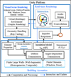Figure 5 Flow diagram of interactive real-time auralization.

Having the impulse response filter h(t) calculated from the equations in the previous chapter, any input time signal $s\left(t\right)$ can be used in convolution, and the output signal is obtained [4]. Generally, the building acoustical frequency range is defined by one-third-octave-bands ranging from 50 Hz to 5000 Hz. The audible frequency range of human hearing is typically from 20 Hz to 20 kHz. In signal processing terms, these quantities have to be turned into frequency spectra with a practical number of frequency lines for auralization [6]. In case of sound insulation filters, an input with 21 values is normally given in building acoustics frequency range (i.e. in one-third octave bands from 50 Hz to 5000 Hz). Hence we can obtain a frequency spectrum with 4097 spectral lines (frequency bins) by using suitable interpolation techniques, such as cubic spline interpolation. HRTFs and binaural filters in equations (33) and (40) are included to take spatial auditory effects into account. In addition to the spatial impression the presentation of building acoustical signals differ in an important point from other techniques, i.e. the relevance of loudness [6]. The colouration, spaciousness and/or the lateral fraction are important in room acoustical auralization which do not have much variation with the change of level. However, in building acoustics the level and colouration are simultaneously the most important quantity. Therefore, during the reproduction of both the correct absolute level and the relative level between source and receiving rooms the care has to be taken into account for not wasting valuable signal to noise ratio in the signal chain. If the absolute level of the sound signals are to be reproduced, a calibration of the replay chain has to be done, see also [7, 11]. Examples of real-time auralizations are given in supplementary material at YouTube⁴ and ITA Website⁵.

5 Results and discussion

The extended model is validated for a workplace for which two adjacent rectangular rooms are selected as source and receiving rooms. To compare the results for façade sound insulation, a corner room is selected as receiving room with exterior walls as composite walls (i.e. an assembly of different materials) which consist of glass windows.

5.1 Performance of the Algorithm

The real-time sound insulation filtering processes are evaluated in terms of computational costs for each step involved. The latencies are calculated for main algorithm that are involved in offline (initialization or pre-process) and real-time computations. All computations were performed on desktop personal computer featuring an Intel Core i7-7700 CPU @ 3.60 GHz multi-core with 16GB RAM, Windows 7 (64-bit) operating system.

Figure 6 shows the latencies calculated for three main processes, 1) source room updates (i.e. impulse response, transmission coefficients, directivity and position of the source), 2) receiver room updates (i.e. impulse response, HRTF and position of the receiver) and 3) building acoustic filters updates (simultaneous source and receiver room updates, and transmission coefficients). In case of adjacent room simulations, the direct partition and flanking walls are segmented into four number of patches (2 × 2). For outdoor case each window (total four) is taken independent patch element. The building acoustic filters update process includes both the source and receiver updates simultaneously. The pre-process includes virtual geometry handling, sound insulation metric calculations and room impulse response synthesis which we need for initialization of auralization properties and the dimensions are not changed during the auralization. The second process is performed in real time which starts with computation of energies hitting at the surfaces of each element $i$ of source room that may vary with the change in position and orientation of the source. The next step is updating the source room impulse responses for each element $i$ and the receiver room impulse responses for each secondary source, and handling of multiple secondary sources with HRTF due to the change in receiver orientation. As the latencies are below the typical threshold of 50 ms [4], free movement of the source (e.g. road, rail or air vehicles) and of the receiver (free movement of the human listener in the virtual receiving room) is validated to be possible without violating real-time performance in interactive Virtual Reality applications.

Figure 6 Latencies for the interactive and real-time source, receiver and filter updates, and comparison of indoor and outdoor example scenes.

5.2 Comparison of standardized level difference D_nT (adjacent rooms)

The purpose of this comparison is to primarily validate the extended method in compliance with the standard prediction models. The indoor scene has source and receiving rooms with dimensions 4 × 4.8 × 3 m³, as shown in Figure 4. The main partition between the offices is 3 × 5 m concrete wall with thickness of $120 \mathrm{mm}$, density $2200\frac{\mathrm{kg}}{{\mathrm{m}}^3}$ and the internal loss factor is 0.005 [9]. To reproduce the results from extended approach, the D_nT values are obtained from the simulated sound pressure values for five different source and receiver positions including the normalization to the reverberation time of the receiving room. This can be interpreted as “virtual measurement” following standard settings [27].

Figure 7 shows the computed D_nT values in one-third octave band which are averaged over five random source positions and five random receiver positions. In the same figure, the predicted D_nT results following ISO 12354-1 (i.e. based on transmission coefficient τ) are compared with that of the extended approach D_nT results. The differences between $D_{\mathrm{nT}}$ values of both ISO and extended approach are also shown. From Figure 7, as we can see that the extended model results are in good agreement with that computed from ISO (i.e. diffuse field approximations) in the case of adjacent rooms. The maximum difference between D_nT values of both approaches is below 1.9 dB. Furthermore, in Figures 8 and 9 it is compared the actual sound insulation of non-standard settings in a real building situation.

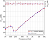Figure 7 Validation of standardized level difference, $D_{\mathrm{nT}}$ calculated from extended approach and ISO 12354-1 between source and receiving rooms (all transmission paths) based on standard settings of source and receiver.

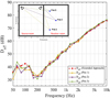Figure 8 Comparison of standardized level differences $D_{\mathrm{nT}}$ between source and receiving rooms (all transmission paths) for Case-I of non-standard configuration settings for the source.

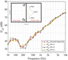Figure 9 Comparison of standardized level differences $D_{\mathrm{nT}}$ between source and receiving rooms (all transmission paths) for Case-II of non-standard configuration settings for the source.

This can be any condition outside the prerequisites for the definition of sound insulation, such as 1.5 m distance between source and receiver positions and room boundaries or source directivities. For this we take two cases as non-standard settings (i.e. source/receiver configurations), where the source is modelled as a HiFi stereo sound system with typical loudspeakers’ directivity, pointing to the centre of the source room. In first configuration, the system is placed 0.3 m away from the flanking walls and in the second configuration it is placed 0.3 m away from one of the partition wall pointing towards centre of the room. The receiver is placed at three random positions in the receiving room.

The resulting D_nT curves for both configurations (Figure 8 and Figure 9) of the system are compared with the standard D_nT values determined for the same sound power but omnidirectional radiations from a standard source position which is greater than 1.5 m from the source room boundaries, which we referred as “virtual measurements” in Figure 7 (red colour plot: D_nT (standard average)). Differences of up to $5 \mathrm{dB}$ are observed in $D_{\mathrm{nT}}$ values of three receiver positions, which are caused by proximity to the room boundaries and source directivities.

5.3 Comparison of standardized level difference D_nT (outdoor sources)

Figure 10 compares the $D_{\mathrm{nT}}$ values of extended approach and diffuse field approximation (ISO) presented for façade sound insulation of an office room with dimensions of 6.5 × 4 × 3 m³. The selected external wall (i.e. façade) of this office is an assembly of different materials and consists of glass windows connected through concrete pillars as shown in Figure 5.

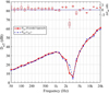Figure 10 Validation of standardized level difference, $D_{\mathrm{nT}}$ calculated from extended approach and ISO between source and receiving rooms (all transmission paths) based on standard settings of source and receiver.

The height and width of each glass window are 2.5 m and 1 m respectively. The glass thickness is 8 mm, density is $2500\frac{\mathrm{kg}}{{\mathrm{m}}^3}$, and the internal loss factor is $0.004$ (0.003 to 0.006 [22]). Each window is a secondary sound source for the receiving room and the sound insulation for each secondary source is computed independently as finite segment. In this way, the façade acts as an assembly of multiple secondary sound sources which radiate sound energy to the receiver room. It is assumed that the sound transmission of each secondary source is independent from the sound transmissions of others and have no interaction with each other in terms of transmission of bending waves across them. The flanking walls are concrete walls in the same setting as in section 5.2 above. Figure 10 compares the $D_{\mathrm{nT}}$ values and its differences $\Delta D_{\mathrm{nT}}$ in dB, computed from diffuse field approximation (ISO 12354-3) and from the extended approach with the standard setting in “virtual measurement”. The procedure to obtain the $D_{\mathrm{nT}}$ values as “virtual measurement” at exactly $45°$ incident angle on the façade the condition of a plane wave incident is fulfilled by placing source at a very large distance (500 m) to the façade and the outdoor sound level is obtained at façade ($L_1$). The indoor sound level ($L_2$) from extended approach is calculated by taking the average sound pressure level for five random positions in the receiving room from all secondary sources (i.e. windows). The reference outdoor $D_{\mathrm{nT},45°}$ referred in blue curve of the Figure 10, is calculated based on [10]. The differences between extended approach and ISO standard $D_{\mathrm{nT}}$ values are also shown in Figure 10, which are in the order of magnitude of $0.6 \mathrm{dB}$ in average with a maximum of $9 \mathrm{dB}$ around $3150$ Hz.

Once the $D_{\mathrm{nT}}$ values from the model are validated and are found in good agreement with standard (ISO) results, we create three example cases with non-standard settings of an outdoor sound source to evaluate the effects of source positions and orientations in front of the façade. This evaluation is performed to realize how big these changes are in effective $D_{\mathrm{nT}}$ values in the receiving room in case of moving outdoor directional sources.

In first example case, the sound source is taken as omnidirectional source (without considering its directivity), while for second and third example cases the sound source is taken as directional source. Figure 11, compares the results of $D_{\mathrm{nT}}$ values for an omnidirectional source placed at four different positions. Figure 12 and Figure 13 compare the results for second and third cases configuration settings such that in Figure 12 a directional sound source is placed at four different positions facing towards perpendicular direction (at 90°) from the façade, while in Figure 13 the source is placed at the same positions, however, facing towards the façade. As an example, a typical source directivity of loudspeaker is selected for the directional sound source as shown in Figure 2.

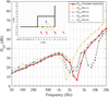Figure 11 Case I: Non-standard configurations with omnidirectional source: Comparisons of standardized level differences $D_{\mathrm{nT}}$ between source and the receiving room.

Figure 12 Comparisons of standardized level differences $D_{\mathrm{nT}}$ between source and the receiving room for Case II of non-standard configurations (with directional source facing 90° away from façade).

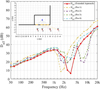Figure 13 Comparisons of standardized level differences $D_{\mathrm{nT}}$ between source and the receiving room for Case III of non-standard configurations (with directional source facing towards façade).

5.4 Sound fields (receiver room) from outdoor excitation

In previous section the $D_{\mathrm{nT}}$ values were compared for different source configurations and non-standard settings. As concerns the sound transmission as such, the source directivity does not play a large role. The main difference is due to the angle-dependent transmission coefficients for different positions in all three cases. However, from interactive and real-time auralization perspective the source power and orientations are required as reference rather than the incident intensity on the façade. Finally, the spatial distribution of the sound pressure level in the receiving room for excitation from outdoor sources is visualized. Three random positions of the sound source are selected. As expected, the outdoor sources have more influence on variation of angle-dependent incident sound power on the building elements and in consequence, on the different amount of energy transmitted through direct path as shown in Figure 14.

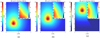Figure 14 Sound pressure level of outdoor source from façade to receiving room at z = 1.5 m, height from floor for three random source positions in a, b and c.

6 Conclusion

In this paper, a model for real-time auralization of sound insulation is introduced by taking into account the source as well as receiving room acoustics with more detailed information. The results of spatial variation of sound pressure inside the receiver room are presented using the knowledge of sound propagation theory in closed spaces for indoor and outdoor cases. Room impulse responses are synthesized from one-third octave band values of the reverberation times and the mean free path in order to incorporate the reverberation effects in accordance with the absorption and geometries of the rooms. Therefore, the aim has been to develop a model that produces more realistic loudness, colouration and binaural impression of the sound transmission at the receiving end by the sound source directivities and source and receiver positions in real-time also for interactive Virtual Reality scenes. However this has not yet been evaluated in subjective experiments. In addition, considering building elements as secondary sources might be helpful to include a more realistic directional cue of sound sources. Although the model presented here is rather detailed in terms of structural-acoustics input data, the claim of the model is not to predict all kinds of existing building elements. In any case, measured sound transmission coefficients from test facilities may serve as input, so that existing (real) building situations can be simulated and compared with measurements. As the model and its open source software is open for any kind of input data, improvements and extensions for more construction types can be implemented easily. The only missing feature in existing standard prediction models (ISO) is the angle dependence, for which a specific solution for monolithic elements is used.

The results of real-time performance of the algorithm in terms of latencies make it possible to render the sound insulation modelled by secondary sources. The results of sound transmission into the receiving room based on diffuse sound field assumptions are compared with that obtained from this model. Under conditions which match the measurement standards of sound insulation testing, the results of the auralization could be validated to differ not more than on average 0.6 dB and 0.3 dB for outdoor and indoor source positions respectively. It is shown that in the results of the extended model, the source directivity and position have an influence on the transmitted energy to the receiving room and, thus, in turn the spatial variation of sound pressure level is more specifically related to the actual scenario and more valid when it comes to auralization. This fact is more obvious in the case of outdoor sound propagating to the receiver room through façades, where we can see that the secondary sources which are more exposed to incident sound field transmit more energy to the receiver room. Furthermore, along this work it is presented a complete building acoustics auralization software framework integrated with virtual reality using audio-visual technology for full open access.⁶ The final goal is to provide a VR system for research, consulting and psychoacoustic assessment of the impact of noise in buildings on humans in an ecologically valid manner.

Conflict of interest

The authors declared that they have no conflict of interest.

Acknowledgments

This work is funded by HEAD-Genuit Foundation under Project ID: <P-17/4-W>. The authors are very grateful for the reviewers’ comments.

References

All Figures

	Figure 1 Example of typical adjacent source and receiving rooms.
In the text

	Figure 2 Sound source directivities for a trumpet and a loudspeaker [16].
In the text

	Figure 3 Example of typical adjacent source and receiver rooms with patches on the walls.
In the text

	Figure 4 Example of a synthetic room impulse response (source room in Fig. 3 is taken as an example room for room impulse response synthesis).
In the text

	Figure 5 Flow diagram of interactive real-time auralization.
In the text

	Figure 6 Latencies for the interactive and real-time source, receiver and filter updates, and comparison of indoor and outdoor example scenes.
In the text

	Figure 7 Validation of standardized level difference, $D_{\mathrm{nT}}$ calculated from extended approach and ISO 12354-1 between source and receiving rooms (all transmission paths) based on standard settings of source and receiver.
In the text

	Figure 8 Comparison of standardized level differences $D_{\mathrm{nT}}$ between source and receiving rooms (all transmission paths) for Case-I of non-standard configuration settings for the source.
In the text

	Figure 9 Comparison of standardized level differences $D_{\mathrm{nT}}$ between source and receiving rooms (all transmission paths) for Case-II of non-standard configuration settings for the source.
In the text

	Figure 10 Validation of standardized level difference, $D_{\mathrm{nT}}$ calculated from extended approach and ISO between source and receiving rooms (all transmission paths) based on standard settings of source and receiver.
In the text

	Figure 11 Case I: Non-standard configurations with omnidirectional source: Comparisons of standardized level differences $D_{\mathrm{nT}}$ between source and the receiving room.
In the text

	Figure 12 Comparisons of standardized level differences $D_{\mathrm{nT}}$ between source and the receiving room for Case II of non-standard configurations (with directional source facing 90° away from façade).
In the text

	Figure 13 Comparisons of standardized level differences $D_{\mathrm{nT}}$ between source and the receiving room for Case III of non-standard configurations (with directional source facing towards façade).
In the text

	Figure 14 Sound pressure level of outdoor source from façade to receiving room at z = 1.5 m, height from floor for three random source positions in a, b and c.
In the text

References

- B. Rasmussen: Harmonization of sound insulation descriptors and classification schemes in Europe: COST Action TU0901, in Proceedings of European Symposium on Harmonisation of European Sound Insulation Descriptors and Classification Standards. 2010. [Google Scholar]
- A. Liebl, H. Jahncke: Review of research on the effects of noise on cognitive performance 2014–2017, in 12th ICBEN conference on noise as a public health problem, 18–22 June 2017, Zurich, Switzerland. 2017. [Google Scholar]
- V. Hongisto, J. Varjo, H. Leppämäki, D. Oliva, J. Hyönä: Work performance in private office rooms: The effects of sound insulation and sound masking. Building and Environment 104 (2016) 263–274. [Google Scholar]
- M. Vorländer: Auralization: fundamentals of acoustics, modelling, simulation, algorithms and acoustic virtual reality. 2nd ed. Springer Nature Switzerland AG, 2020. [Google Scholar]
- M. Vorländer, R. Thaden: Auralization of airborne sound insulation in buildings. Acta Acustica united with Acustica 86, 1 (2000) 70–76. [Google Scholar]
- R. Thaden: Auralization in building acoustics. PhD dissertation, RWTH University Aachen. Germany, 2007. [Google Scholar]
- S.J. Schlittmeier, J. Hellbrück, R. Thaden, M. Vorländer: The impact of background speech varying in intelligibility: Effects on cognitive performance and perceived disturbance. Ergonomics 51, 5 (2008) 719–736. [CrossRef] [PubMed] [Google Scholar]
- A. Rodríguez-Molares: A new method for auralization of airborne sound insulation. Applied Acoustics 74, 1 (2013) 116–121. [Google Scholar]
- ISO EN 12354-1: Building acoustics: estimation of acoustic performance of buildings from the performance of elements – Part 1: airborne sound insulation between rooms. International Organization for Standardization, Geneva, 2017. [Google Scholar]
- ISO, EN 12354-3: Building acoustics: estimation of acoustic performance of buildings from the performance of elements – Part 3: airborne sound insulation against outdoor sound. International Organization for Standardization, Geneva, 2017. [Google Scholar]
- M. Imran, M. Vorländer, S.J. Schlittmeier: Audio-video virtual reality environments in building acoustics: An exemplary study reproducing performance results and subjective ratings of a laboratory listening experiment. The Journal of the Acoustical Society of America 146, 3 (2019) EL310–EL316. [CrossRef] [PubMed] [Google Scholar]
- O.C. Zienkiewicz, R.L. Taylor, P. Nithiarasu, J.Z. Zhu: The finite element method, Vol 3. McGraw-Hill, London, 1977. [Google Scholar]
- E. Reynders, R.S. Langley, A. Dijckmans, G. Vermeir: A hybrid finite element–statistical energy analysis approach to robust sound transmission modelling. Journal of Sound and Vibration 333, 19 (2014) 4621–4636. [Google Scholar]
- R.H. Lyon, R.G. DeJong, M. Heckl: Theory and application of statistical energy analysis. Butterworth-Heinemann, USA, 1995. [Google Scholar]
- E. Gerretsen: Calculation of the sound transmission between dwellings by partitions and flanking structures. Applied Acoustics 12, 6 (1979) 413–433. [Google Scholar]
- R.H.C. Wenmaekers, C.C.J.M. Hak, M.C.J. Hornikx, A.G. Kohlrausch: Sensitivity of stage acoustic parameters to source and receiver directivity: Measurements on three stages and in two orchestra pits. Applied Acoustics 123 (2017) 20–28. [Google Scholar]
- J.H. Rindel: Sound insulation in buildings. CRC Press, US, 2018. [Google Scholar]
- T.E. Vigran: Building acoustics. CRC Press, London, 2014. [Google Scholar]
- M. Vorländer: Revised relation between the sound power and the average sound pressure level in rooms and consequences for acoustic measurements. Acta Acustica united with Acustica 81, 4 (1995) 332–343. [Google Scholar]
- L. Cremer: Theorie der Schalldämmung Wände bei schrägem Einfall. Akustische Zeitschrift 7 (1942) 81–104. Most of this article has been republished with an English language summary, Northwood, TD: Theory of the Sound Attenuation of Thin Walls with Oblique Incidence. Architectural Acoustics, Benchmark Papers in Acoustics 10, 367–99. [Google Scholar]
- ISO 15712-1:2005(E): Building acoustics – Estimation of acoustic performance of buildings from the performance of elements – Part 1: Airborne sound insulation between rooms. International Organisation for Standardization, Geneva, Switzerland, 2005. [Google Scholar]
- C. Hopkins: Sound insulation. Routledge, 2012 May 31. [Google Scholar]
- J. Davy: Predicting the sound insulation of single leaf walls: Extension of Cremer’s model. The Journal of the Acoustical Society of America 126, 4 (2009) 1871–1877. [CrossRef] [PubMed] [Google Scholar]
- I.S. Gradshteyn, I.M. Ryzhik, in Table of Integrals, Series, and Products, prepared by Yu. V. Geronimus and M. Yu. Tseytlin, translated from Russian by Scripta Technica Inc., 4th ed., Jeffrey A., Editor. New York: Academic, 1965. [Google Scholar]
- J. Davy: The radiation efficiency of finite size flat panels, in Annual Conference of the Australian Acoustical Society. Australian Acoustical Society, 2004. [Google Scholar]
- M. Imran, A. Heimes, M. Vorländer: Sound insulation auralization filters design for outdoor moving sources, in Proc. 23rd International Congress on Acoustics, Aachen, 2019, pp. 283–288. [Google Scholar]
- ISO, EN. 10140-2: Acoustics: Acoustics-Laboratory measurement of sound insulation of building elements – Part 2: Measurement of airborne sound insulation. International Organization for Standardization, Geneva, 2010. [Google Scholar]
Cite this article as: Muhammad I, Heimes A & Vorländer M. 2021. Interactive real-time auralization of airborne sound insulation in buildings. Acta Acustica, 5, 19.