| Issue |
Acta Acust.
Volume 9, 2025
Topical Issue - Vibroacoustics
|
|
|---|---|---|
| Article Number | 12 | |
| Number of page(s) | 18 | |
| DOI | https://doi.org/10.1051/aacus/2024088 | |
| Published online | 17 February 2025 | |
Scientific Article
Acoustic absorption of 3D printed samples at normal incidence and as a duct liner
1
Ecole Centrale de Lyon, CNRS, Universite Claude Bernard Lyon 1, INSA Lyon, LMFA, UMR 5509, 69130 Ecully, France
2
Institute of Fundamental Technological Research, Polish Academy of Sciences, ul. Pawińskiego 5B, 02-106 Warsaw, Poland
* Corresponding author: This email address is being protected from spambots. You need JavaScript enabled to view it.
Received:
14
May
2024
Accepted:
9
December
2024
Abstract
Prediction of the acoustic performance of 3D printed materials is investigated at normal and grazing incidence. A direct numerical (microscopic) simulation that solves the full set of Navier–Stokes equations is used as a reference. It is compared with a macroscopic approach in which the material is represented by an equivalent fluid. The materials have a periodic microstructure, consisting either of a single network of spherical or cubic cavities connected by cylindrical channels or of a double-nested network. The samples are printed using the stereolithography technique and are tested using an impedance tube and a duct test bench. For single network geometries, the results of sound absorption at normal and grazing incidence predicted using the equivalent fluid approach are in good agreement with those obtained by the microscopic approach. Comparisons with impedance tube measurements confirm that both approaches can accurately predict the absorption coefficient of the samples. For the in-duct liner configuration, the transmission loss measurements and predictions show similar evolution with frequency change, despite the discrepancy in amplitude. For the double network geometry, the equivalent fluid approach cannot exactly reproduce the results obtained with the direct numerical simulation. Finally, while the predictions with the microscopic approach provide a good match with the impedance tube measurements, only a poor agreement is obtained using the duct testing bench.
Key words: Acoustic absorber / 3D printing / Duct / Multiscale approach
© The Author(s), Published by EDP Sciences, 2025
 This is an Open Access article distributed under the terms of the Creative Commons Attribution License (https://creativecommons.org/licenses/by/4.0), which permits unrestricted use, distribution, and reproduction in any medium, provided the original work is properly cited.
1 Introduction
Recently, advances in 3D printing techniques have been effectively used in research on noise reduction systems involving, in particular, acoustic metamaterials, as these modern manufacturing technologies enable realization of geometries that are difficult to produce with traditional manufacturing processes. There are many examples of 3D printed acoustic materials in the literature, but only some of them, such as space-coiling geometries [1, 2] labyrinthine channels in microporous skeletons [3], extended neck Helmholtz resonators [4, 5], and coupled or detuned resonators [6, 7], may achieve impressive absorption properties. The ease of use and affordability of 3D printing techniques could allow one to manufacture tailored sound absorbers that meet specific requirements in the near future. This challenging but reachable goal requires two prerequisites. First, it is necessary to ensure the reliability of the dimensions obtained during the production of absorbent structures. Secondly, one should be able to accurately predict the absorption properties of a variety of geometries, and do so in different configurations. In the present work, we focus on this second aspect.
Two main approaches are used to predict the absorption properties of rigid and motionless materials. The first one are direct methods that describe sound propagation at the pore scale. In particular, direct numerical simulations solve the full set of Navier–Stokes equations inside the sample and account accurately for thermo-viscous losses. They are straightforward but require significant computational resources, which make them inefficient for extensive parametric studies. The second approach are the macroscopic methods that model the material at the system scale. These include surface impedance and equivalent fluid models. These methods are much more efficient, but are less general than the direct microscopic simulations. Thus, surface impedance models are appropriate for locally-reacting materials, but fail otherwise. Equivalent fluid models are more relevant for extended-reacting materials. However, they require that the following assumptions are met: (i) the existence of a periodic unit cell a.k.a. a representative elementary volume (REV) in the microstructure of the material,(ii) wavelengths larger than the REV size, and (iii) a sufficiently large number of REV in the material sample. Note that it is possible to relate the acoustic properties of these macroscopic models to the REV geometry.
Most of the acoustic devices listed in the first paragraph were tested in an impedance tube, which is the basic configuration to assess the sound absorption of materials at normal incidence. For real-world applications, more complex configurations have to be considered. For instance, for room acoustics applications, the absorption of the material should be examined using a diffusive field. For ventilation systems, mufflers or nacelles of aircraft engines, grazing incidence is more appropriate than normal incidence. However, there are actually few examples of 3D printed devices that were tested in such configurations. We can refer for a 3D-printed material mounted in the wall of a duct to Oh and Jeon [8] and Boulvert et al. [9, 10], used as a duct termination to Meng et al. [11], or tested in a reverberation room to Nistri et al. [12]. Note that all of these studies concern locally-reacting materials.
The objective of this paper is twofold. First, we want to check whether macroscopic methods can predict the sound absorption properties of 3D printed samples similar to the reference direct numerical simulations performed on the microscale in two different configurations, namely at normal and grazing incidence. Second, we want to compare the respective experimental results and numerical predictions obtained for these two configurations. To do so, we consider 3D printed samples with periodic microstructures based on three different unit cells.
The article is organized as follows. The periodic geometries are described in Section 2. Then, the direct numerical simulation and the equivalent fluid approach are explained in detail in Section 3. Comparison between experimental and numerical results are first shown at normal incidence in Section 4 and then at grazing incidence for the in-duct liner configuration in Section 5. A discussion on these results is proposed in Section 6. Finally, concluding remarks are given in Section 7.
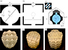 |
Figure 1 (Top) Unit cells for the considered periodic geometries: (a) OPCL, (b) cubic, and (c) DNN. The air-saturated pores are represented in white (and also in blue for the large network of DNN) and the rigid skeleton is in black. (Bottom) Pictures of the corresponding samples 3D printed for testing in a 29 mm impedance tube: (d) OPCL, (e) cubic, (f) DNN. |
2 Periodic geometries of 3D printed materials
All studied materials have a periodic microstructure. Three periodic geometries are considered. Unit cells for the three geometries are presented in Figure 1 along with pictures of the corresponding samples 3D printed for testing in a 29 mm diameter impedance tube. The first two geometries consist of a single network of cavities, that are either cubic or spherical, linked to neighbouring cavities by small cylindrical channels in the three directions in space. The design is inspired by the One-Pore Cell (OPC) geometry of the round-robin study performed in Zieliński et al. [13]. This geometry offers many advantages: it is simple, it can be easily realized with additive manufacturing, and it has several symmetries, that can be used to reduce the computational cost of numerical simulations. In the original OPC geometry, the cell width was of 5 mm, the cavities were spherical with a diameter of 4.5 mm, and the channel diameter was of 2 mm. The absorption coefficient showed several peaks, suggesting a resonant behaviour. The frequency of the first absorption peak was measured at 1000 Hz for a 60 mm height sample. In order to obtain a first peak in the same frequency range but for a smaller sample height, we have modified the dimensions of the cell. The frequency of the first peak has been tuned by shrinking the channels and enlarging the pores and thus increasing the tortuosity of the material. As a result, the frequency of the absorption peak associated with the quarter-wavelength resonance has been lowered. The first studied geometry is thus composed of a cell of 9 mm width, a sphere diameter of 8 mm, and a channel diameter of 1.5 mm. These new dimensions, particularly the channel diameter, also aimed at investigating the limitations of the 3D printing technique used. The unit cell for this geometry, called One-Pore Cell Large (OPCL) hereafter, is sketched in Figure 1a. We have also derived from OPCL a geometry with a cubic cavity in order to increase the porosity of the material, which is referred to as the cubic geometry subsequently (see the unit cell in Fig. 1b). Finally, we have investigated a double nested network (DNN) geometry. For this purpose, we have inserted in the skeleton of the OPCL geometry a second network of spherical cavities. Both networks are independent, i.e. they are not connected to each other. In the first network, referred to as the “large” subnetwork, the cavity diameter is 8.5 mm and the channel diameter is 1.2 mm. In the second network, referred to as the “small” subnetwork, the cavity diameter is 6.5 mm and the channel diameter is 2 mm. Figure 1c represents the unit cell along with a sketch of the network structure. In addition to increasing the porosity, the objective is to obtain two peaks of absorption, whose frequencies are close enough to achieve absorption over a wider frequency range. The dimensions of the elementary cells are compared in Table 1. Note that the cell width is identical for the three geometries studied in this work.
Characteristic dimensions of the periodic geometries.
The samples manufactured for the studies at normal and grazing incidence, shown in Figure 2, have a thickness H = 31.5 mm. This corresponds to three full cells and one half cell. This implies that the surface of the samples does not show the same geometrical characteristics on the two sides, as depicted in Figure 3. Thereafter, we refer to “face A” the configuration for which the surface of the sample showing the cavities is facing the acoustic waves and “face B” the configuration for which the surface of the sample showing the channels is facing the acoustic waves.
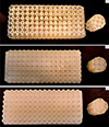 |
Figure 2 Samples for the impedance tube and the duct bench for the geometries OPC (a), cubic (b), and DNN (c). |
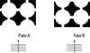 |
Figure 3 Sketch showing the two different faces of the samples. |
The samples are manufactured with a Formlabs Form2 printer. It uses the stereolithography technique, often described in the literature as the most accurate and reliable additive manufacturing technology [13, 14]. The samples are printed with the Formlabs Clear-04 resin using a printing resolution of 0.025 mm which is the highest resolution available on the printer. With this resolution, the details of the geometries can be printed with negligible staircase effect. Therefore, the effect of roughness, which can have a noticeable impact on the acoustic properties of the samples [15], should be small. In addition, the samples manufactured with the stereolithography technique do not exhibit microporosity, contrary to other additive manufacturing techniques such as power bed fusion. Moreover, they are characterized by high quality and accurate geometry reproduction. Nevertheless, the characteristic dimensions of the 3D printed geometries inevitably deviate from their design values, which has an impact on the acoustic properties of the samples [16]. Measurements of the actual dimensions of the samples have been done and are reported in Appendix A.
3 Acoustic modelling of the 3D printed samples
3.1 Microscopic approach using direct numerical simulation
The direct approach to predict the acoustic absorption of the samples is to describe the sample down to the microscopic scale with all the geometric details and to determine sound propagation in the sample. This approach is referred to as direct numerical simulation (DNS). Because of the absence of microporosity and the rigidity of the skeleton, we need to consider only the wave propagation in the air saturating the pores. The solution to this problem is obtained by solving the full set of linearized Navier–Stokes (LNS) equations, that account for coupled thermo-viscous effects which are significant in the pores of thematerial.
We use the convention eiω t . Denoting by p, T, and v the acoustic fluctuations of pressure, temperature and velocity, the linearized Navier–Stokes equation of motion, the conservation of mass equation, and the heat conduction equation read:
 (1)
(1)
 (2)
(2)
 (3)
(3)
where p 0, T 0, and ρ 0 are the equilibrium values of ambient pressure, temperature and density, η is the dynamic viscosity of air, c p is its specific heat capacity at constant pressure, and κ is its thermal conductivity. At the fluid/structure interface, a no-slip condition v = 0 and an isothermal condition T = 0 are applied.
The DNS have been performed using the finite element software COMSOL Multiphysics. This commercial software was used for all numerical simulations of this work. Special attention has been paid to the meshing, in particular to discretize the acoustic boundary layers with a sufficient number of elements.
3.2 Multiscale approach using an equivalent fluid model
The direct numerical solution requires significant computational resources. For most applications (for instance, to optimize the geometry to improve acoustic performance), it is necessary to perform a large number of simulations. In such cases, it is preferable to employ simplified or homogenized models which are far less costly. In such approaches, the details of the microgeometry are not considered directly and the material is considered at the macroscale level. The first approach would be to replace the material by its surface impedance. However, the samples under consideration have an extended reaction behaviour (see Sect. 5.2.1). While modelling the sample by its surface impedance is appropriate at normal incidence, it does not lead to a correct prediction of the acoustic behaviour at grazing incidence [17]. Thus, we consider a second approach in which the sample is modelled at a macroscopic scale with an equivalent fluid.
The equivalent fluid method is commonly used to model classical porous materials which present an open porosity and a rigid skeleton. This description replaces the actual material by an equivalent fluid, with a frequency-dependent density ρ e (ω) and compressibility C e (ω). The equations governing the acoustic wave propagation in the material become:
 (4)
(4)
 (5)
(5)
Based on the homogenization theory, the dynamic functions ρ e and C e can be determined directly by solving for each frequency of interest the harmonic Stokes flow and heat transfer problems in a periodic unit cell representing the geometry on a microscopic scale, called representative elementary volume. This methodology is referred to as a direct multiscale (DM) calculation. Usually, one rather expresses the dynamic functions ρ e and C e using the Johnson-Champoux-Allard-Lafarge-Pride (JCALP) model [18–21]. The eight semi-phenomenological parameters of these dynamic functions can be calculated by solving the Laplace, Stokes and Poisson problems in a REV. This approach is known as the hybrid multiscale (HM) calculation.
Note that the DM and HM approaches are well suited for 3D printed samples with a periodic structure, as considered in this work, because the geometry of the REV is known. In the case of foam and fibrous materials, the REV can be deduced from a microscopic observation of the structure geometry, allowing either the calculation of ρ e and C e or the eight JCALP parameters [22–24].
The homogenization theory assumes that the REV size is small compared to the wavelength and material thickness. This latter hypothesis is not fully verified in our case, because the samples contain only a few cells along their height. However, Zieliński et al. [25] have shown that the behaviour of the same kind of structure can be predicted with an equivalent fluid approach at normal incidence over an acceptable frequency range.
The HM approach is applied for the three geometries, following the procedure detailed in Zieliński et al. [25]. To do so, relevant finite element analyses have been performed on the unit cells using COMSOL Multiphysics. As for the DNS, the mesh has been carefully generated. According to the guidelines given in Zieliński et al. [25], fillets have been applied on sharp edges. The calculated values of the JCALP parameters are reported in Table 2. Note the large increase in porosity and tortuosity for the cubic geometry compared to OPCL. For DNN, three sets of parameters are given. They are calculated for the two subnetworks evaluated separately, i.e. for the “small” subnetwork and then for the “large” one, as well as for the whole DNN unit cell.
JCALP parameters for the OPCL, cubic, and double nested network (DNN) geometries.
4 The case of normal incidence
4.1 Experimental set up and model
The experimental setup for the normal incidence case is a B&K Type 4206 impedance tube kit, with a 29 mm diameter impedance tube. At one end of the tube, a loudspeaker generates a random broadband signal with an amplitude of around 70 dB. The samples are inserted at the other end and placed against a rigid backplate. In order to reduce sound leakage, Teflon adhesive tape has been applied around the samples and on the surface near the hard backing. The pressure is measured using two quarter-inch microphones (B&K Type 4187). The absorption coefficient is then calculated from the frequency response between these two microphones.
The impedance tube configuration for the direct numerical simulation is sketched in Figure 4. The linearized Navier–Stokes equations are solved inside the pore network of the material and also in a small domain near the sample surface to account for potential evanescent waves. The Helmholtz equation is solved in the remaining part of the tube. The computed acoustic pressure is recorded and averaged on two sections of the tube (at the microphone positions 1 and 2) allowing the calculation of the absorption coefficient. For reducing computational cost, the cross section of the impedance tube only contains a quarter cell and symmetry boundary conditions are applied to obtain full 3D results.
 |
Figure 4 Sketch for the DNS of the impedance tube testing. The pressure is averaged on the two surfaces represented by the red lines at the positions of the microphones 1 and 2. |
For the multiscale approach, the absorption coefficient is calculated analytically for configurations in which the sample is represented by an equivalent fluid. For DNN, we represent in some configurations the sample by two equivalent fluids. In such cases, a numerical simulation is performed and the equivalent fluid equations are solved in the sample.
The DNS for 300 frequency steps lasts 6.5 h on 6 compute nodes of 16 cores. The finite element mesh contains 60 000 elements. Due to the large number of degrees of freedom (DoF), a memory with a capacity of 384 GB has to be used. For comparison the calculation of the JCALP parameters from the unit cell takes only a few minutes on a desktop machine and the analytical computation of the absorption coefficient is practically instantaneous. The numerical simulation for the impedance tube with the equivalent fluid equations also takes a few minutes when performed on a desktop machine. This suggests the use of the multiscale approach to characterize these materials even in the simple case of normal incidence.
4.2 Comparisons of modelling results
4.2.1 Results for single network materials
Figure 5 presents the absorption coefficient calculated from two computationally demanding direct numerical simulations (i.e. for the “face A” and “face B” configurations) and using the equivalent fluid method. Note that the results are shown for frequencies between 400 Hz and 2400 Hz, corresponding to the frequency range that is of interest for the duct application, cf. Section 5.
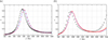 |
Figure 5 Absorption coefficient for the OPCL geometry (a) and the cubic geometry (b): results from the equivalent fluid model (——) and from two direct numerical simulations, i.e. for the “face A” (+) and “face B” (+) configurations. |
For all cases, the absorption coefficient shows a single peak in this frequency range. Considering the results from the DNS, one observes that the absorption coefficient is slightly different for the two material configurations (i.e. “face A” and “face B”). This can be explained by the added length effects occurring due to the small cylindrical channels at the sample surface in the “face B” configuration.
The equivalent fluid approach provides an absorption curve that is nearly identical with the curve calculated for the “face A” configuration using the direct numerical simulation. Note that a length correction [26] can be applied when using the equivalent fluid method to account for the added length effects present in the “face B” configuration. This would result in a small increase in the tortuosity that shifts the peak frequency of the absorption coefficient calculated by the equivalent fluid approach towards a lower frequency corresponding to the “face B” configuration.
Although not shown in the graphs as this is outside the frequency range of interest, the curves calculated by DNS and the equivalent fluid method diverge at high frequencies, starting from 3000 Hz for the OPCL geometry and 2500 Hz for the cubic geometry. This can be explained by the long-wavelength assumption of the equivalent fluid approach. Indeed, the characteristic size of the representative elementary volume, corresponding to the cell size, must be small compared with the wavelength. For a frequency of 3000 Hz, the wavelength in air is less than 12 cm which is only an order of magnitude higher than the cell size (0.9 cm), and moreover, wavelengths are shorter in a porous rigid-frame material saturated with air than in free air. This sets the limit for using the equivalent fluid approach for this geometry.
In addition, note that the two absorption peaks visible in Figure 5 (one for the OPCL layer and the other for the cubic pore network) are the result of the so-called quarter-wavelength resonances. To see more such resonances, the two absorption curves, determined using the equivalent fluid models for the OPCL and cubic-pore layers, respectively, are presented in Figure 6 in a wider frequency range, i.e. from 100 Hz to 5 kHz. In addition, Figure 6b shows a graph where the same absorption curves are re-plotted against a dimensionless parameter instead of frequency f [27, 28]. The dimensionless parameter is defined as the ratio of the layer thickness H to a quarter of the wavelength, i.e. 4H/λw. Note that the wavelength λw-pagination is associated with the effective speed of sound ce in the porous material considered, namely λw(f)=Re[ ce(f)]/f, where Re denotes the real part. It is completely different from the wavelength in the air, especially at lower frequencies. It also differs significantly between the OPCL and cubic-pore networks. Now, it is easy to see that absorption peaks occur when 4H/λw = 1, 3, 5, etc. In the frequency range below 5 kHz, there are three such peaks in the case of the cubic-pore layer, at approximately f1 = 949 Hz, f3 = 2914 Hz, and f5 = 4893 Hz, while only two absorption peaks for the OPCL layer of the same thickness, i.e. due to the quarter-wavelength resonance at f1 = 1220 Hz and the three-quarter-wavelength resonance at f3 = 3732 Hz (see Fig. 6).
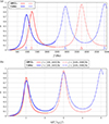 |
Figure 6 Sound absorption coefficient α for the hard-backed layer of the OPCL material (red curves) or cubic pore network material (blue curves) versus: (a) frequency f, or (b) 4H/λ w(f) where H is the layer thickness and λ w is the wavelength in the respective equivalent fluid. |
The frequencies of the absorption peaks can be tuned by changing the layer thickness or by tailoring the pore network geometry. The second approach involves, for example, enlarging the pores and shrinking the channels that link them. In that way, the tortuosity of the porous material is increased while the viscous characteristic length and permeability are reduced. As a result, the effective speed of sound in the fluid equivalent to the air-saturated porous medium is slowed down, which means that the effective wavelength at each frequency is shortened. As demonstrated in Figure 6, the peak in sound absorption occurs when a quarter (three-quarters, five-quarters, etc.) of the wavelength is equal to the thickness of the material. The frequencies of such quarter-wavelength resonances can be lowered in that way, and eventually tuned to the required values since the opposite effect (i.e. decreasing the tortuosity and therefore raising the resonance frequencies) is achieved by widening the channels and/or reducing the pore size.
4.2.2 Results for a double nested network material
The absorption coefficient for DNN determined from the direct numerical simulation and from the multiscale approach is shown in Figure 7b for the two faces configuration of the sample. The geometry (spheres or channels) of the large network visible at the sample surface is taken as a reference to distinguish the two configurations (see Fig. 7a). Compared to the single network geometries, the absorption coefficient for DNN determined with DNS shows two peaks in the frequency range of interest. Thus, we can observe the wider absorption frequency bandwidth obtained with these two detuned networks. Note that the first peak is shifted towards low frequencies for the “face B” configuration compared with the “face A” configuration, and vice versa for the second peak.
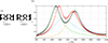 |
Figure 7 (a) Sketch of the two faces configurations considered for the DNN geometry. (b) Absorption coefficient determined with the direct simulation for the “face A” (+) and “face B” (+) configurations and using the equivalent fluid method with a single equivalent fluid corresponding to the large (--), small (--), or double network (--). |
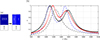 |
Figure 8 (a) Sketch of the finite element model for the multiscale approach using two equivalent fluids. (b) Absorption coefficient determined with the direct simulation for the “face A” (+) and “face B” (+) orientations and using the multiscale approach with two equivalent fluids for the “separated” (--) and “contiguous” ( |
For the multiscale approach, we first model the sample as a single equivalent fluid using the set of JCALP parameters obtained either for the large or small subnetworks or for the full DNN cell (see Tab. 2). In all three cases, the absorption coefficient has a single peak in the considered frequency range, see Figure 7b. Each of these three peaks is centred at a different frequency depending on the JCALP parameters used. Recall that the absorption curve calculated by DNS has two absorption peaks, and it is now easy to notice that the first of them is related to the large network while the second peak coincides with the small network. Finally, the sound absorption curve calculated using the equivalent fluid for the full unit cell tends to be a rough average of those obtained for the large and small networks.
Therefore, it seems that a single equivalent fluid is not suitable to predict the acoustic properties of DNN made of two independent networks. Thus, we have tried an alternative model of the sample in which we have used two different equivalent fluids for each of the networks. As sketched in Figure 8a, each equivalent fluid fills half of the sample volume. Since the subnetworks are independent, it appears appropriate to separate the two fluids with a rigid wall. This configuration is called the “separated” configuration and the corresponding absorption coefficient is plotted in Figure 8b, along with the reference DNS results. It can be noted that this approach allows one to predict the presence of two peaks and their frequencies, but do not provide an accurate prediction of the absorption coefficient for either face of the sample. This discrepancy could be linked with an evanescent coupling between the two networks at the surface of the sample. In addition, as the realization of the samples is not perfect, acoustic information could be transmitted from a subnetwork to the other. This could happen by external communication due to leakage around the samples or at its end. This could also occur by internal communication due to transmission through the thin walls of the inner geometry, or due to an imperfect realization that would connect the two networks. This is the reason why we have tested another configuration denoted “contiguous” in which the continuity of pressure and normal velocity is ensured at the interface between the two equivalent fluids. The absorption coefficient for this configuration is also plotted in Figure 8b. A single peak is observed. The result is quite similar to the one for the unique equivalent fluid of the full cell presented in Figure 7, but with a higher amplitude. This different behaviour between the “separated” and the “contiguous” configurations imply that the realization of the sample and its mounting in the impedance tube are of crucial importance to observe two peaks for the absorptioncoefficient.
4.3 Comparison with measurements
Figure 9 presents the absorption coefficient obtained from the measurements and from the direct simulation for the two facing orientations of the samples, i.e. “face A” and “face B”. The three graphs show the results obtained for: (a) the OPCL geometry, (b) the cubic geometry, and (c) the double nested network. We can observe that the absorption coefficient is well predicted for the two single network geometries. In particular, the difference in behaviour for the two faces of the samples is accurately reproduced by the numerical simulations. Furthermore, the shift of the peak towards lower frequencies for the cubic geometry compared to the OPCL geometry is also found experimentally. However, one observes that the peaks of the measured absorption curves are higher and centred at lower frequencies than predicted from numerical simulations. These differences between the measurements and the predictions can be attributed to sound leakage around the samples [29], samples imperfections, and slight differences between the design and the manufactured geometries [16]. Concerning the double-nested network, the absorption coefficient determined from the experiments shows two peaks for the “face A” configuration. Compared to the numerical predictions, the peaks appear at lower frequencies, as for single network geometries. In addition, the width of the peaks is much larger, resulting in a larger absorption bandwidth. For the “face B” orientation of the sample, a single broad peak (or rather a plateau formed between two peaks) can be observed in the experiments. As the frequencies of the two peaks are closer for the “face B” than for the “face A” configuration in the DNS, this single peak in the experiments can be interpreted as the merging of the two wide peaks forming a nearly-perfect absorption bandwidth between 1 kHz and 1.5 kHz.
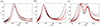 |
Figure 9 Absorption coefficient for geometries OPCL (a) cubic (b), and DNN (c) obtained from the direct simulation for the “face A” (+) and “face B” (+) configurations and from the measurements for the “face A” (—) and “face B” (—) orientations. |
5 The case of grazing incidence
5.1 Experimental set up and models
The experimental setup used to measure the acoustic performance of the samples in a duct wall is the MATISSE testing bench at LMFA which has been used in previous studies [30, 31]. It is sketched in Figure 10a. The duct has a square cross-section (66 mm × 66 mm) and its cut-off frequency is about 2.5 kHz, implying that only plane waves propagate below this frequency. A loudspeaker placed above the duct generates a broadband random noise with an amplitude of around 80 dB. Pressure is measured at four points using four quarter-inch B\AMP K microphones, two of which (i.e. microphones 1 and 2) are located in the front of and two (i.e. microphones 3 and 4) behind the lined section of the duct, see Figure 10. The length of each of the samples is L = 150 mm, and they are adapted to the duct with a dedicated sample holder. As for the samples in normal incidence, Teflon adhesive tape has been applied on the surface of the samples to reduce leakage.
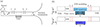 |
Figure 10 (a) Sketch of the MATISSE bench. (b) Configuration for the numerical simulations for: (top) the DNS and (bottom) for the equivalent fluid approach. |
The transmission loss (TL) is used to characterize the acoustic performance of the 3D printed materials as duct liners. It is defined as the ratio of the incident power to the transmitted power after the lined section [32]. Under plane wave excitation, it can be estimated from the pressure at the four microphones.
In order to evaluate the usability and accuracy of the equivalent fluid model for the in-duct configuration and for comparison with experimental results, two different numerical models of the lined duct, corresponding to the direct microscopic and multiscale approaches, are realized. The respective configurations are presented in Figure 10b. An incident plane wave, with an amplitude p ind = 1 Pa, is generated upstream of the acoustic treatment. At both ends of the duct, perfectly matched layers are used to simulate non-reflecting boundary conditions. The pressure is evaluated at the position of the four microphones for the calculation of the transmission loss. Apart from the lined section, the duct walls are rigid. For the direct microscopic approach, the geometry at the cell size is reproduced. To limit the computational cost, only half a cell is considered in the y-direction and symmetry conditions are applied to obtain the full 3D behaviour. The LNS equations are solved in the pore network of the material and in a small domain above the sample to capture thermo-viscous effects near the liner surface. In the remaining part of the duct, the Helmholtz equation is solved. For the multiscale approach, the liner is replaced by an equivalent fluid using the JCALP parameters determined from the microstructure and presented in Section 3.2. Then, a three-dimensional simulation at full scale is performed in which the Helmholtz equations are solved in the liner modelled as an effective fluid and in the air in the duct.
In terms of computational resources, the difference between the two approaches is significant and even greater than for the impedance tube calculations. The DNS requires a memory of above 1 TB with over one million mesh elements and the CPU time is 10 h, whereas the multiscale approach is performed on a desktop machine in about 10 min.
5.2 Results for single network samples
5.2.1 Comparison of modelling results
Figure 11 shows the TLs obtained for the OPCL and cubic geometries using the direct simulation and the equivalent fluid approach. The conclusions for the case of grazing incidence are consistent with those at normal incidence. Thus, for the microscopic approach, it is found that the transmission loss depends on which face of the sample placed in the duct wall is facing the inside of the duct. As for the absorption coefficient, the TL peak is shifted towards a lower frequency when “face B” is on the top of the liner, compared to “face A” orientation. Furthermore, note that the TL determined with the equivalent fluid approach matches closely the results obtained from DNS performed for the “face A” configuration.
 |
Figure 11 Transmission loss for the OPCL (a) and cubic (b) geometry: equivalent fluid approach ( |
Comparing the two graphs in Figure 11 the TL peaks appear at lower frequencies for cubic geometry than for OPCL geometry. The same regularity has already been observed for the absorption coefficient in Figure 5. Finally, the amplitude of the TL peak for “face A” orientation is lower for the cubic geometry than for OPCL.
To illustrate the close correspondence between the direct microscopic and multiscale approaches for the “face A” configuration, Figure 12 compares the normalized pressure modulus inside the material and in the duct calculated for the OPCL and cubic geometries at the frequency of the TL peak, using DNS or equivalent fluid model. The equivalent fluid approach faithfully reproduces the acoustic pressure field inside the pores of the material predicted with DNS. Note also that the variations in the pressure inside the sample suggest the existence of a longitudinal mode, with maxima along the duct walls and a nodal line in the middle of the duct. This behaviour is typical of an extended-reacting liner. It can be observed in Figure 12 that the sample is not symmetric in the direction of the duct axis. Tests have been performed both numerically and experimentally and have shown that the TL is almost identical when the sample is rotated by 180°.
 |
Figure 12 Map of the acoustic pressure modulus |p|/pind for the OPCL (a) and cubic (b) geometry for the “face A” orientation at the frequency of the TL maximum, (i.e. f = 1240 Hz (a) and f = 980 Hz (b)): direct simulation (top) and equivalent fluid model (bottom). |
5.2.2 Comparison with measurements
Figure 13 compares the TLs measured and predicted for the OPCL geometry. As for the DNS, the measured TLs show a single peak, which is centered at a lower frequency for the “face B” orientation than for the “face A” orientation. For “face A”, the frequency of the peak is in good agreement between the DNS and the measurements. However, for “face B”, the peak of the measured TL is observed at lower frequency than predicted. Overall, the peaks in the measured TL curves are “rounded” and suppressed compared to the predictions. As a consequence, the maximum of TL is largely reduced in the experiments. Thus, e.g., the peak for the “face A” configuration reaches 10 dB in the experiments and 27 dB in the results predicted by DNS.
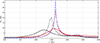 |
Figure 13 Transmission loss for the OPCL geometry modelled with the equivalent fluid approach ( |
The same comparison is performed for the cubic geometry in Figure 14. This time, good agreement between the predictions and the experimental results is observed. In particular, the predicted frequency and the width of the peak for both orientations of the sample are confirmed by the experiments. For “face B”, the peak value found in the experiments (around 18 dB) is also close to that predicted by DNS (around 25 dB). On the other hand, the peak value found experimentally for “face A” is almost 45 dB, which is much higher than 18 dB predicted by DNS; this very sharp peak with such a large value of TL is an unexpected result, which is uncommon in the measurements reported in the literature.
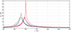 |
Figure 14 Transmission loss for the cubic geometry modelled with the equivalent fluid approach (––) and with the direct numerical simulation for the “face A” ( |
5.3 Results for a double nested network sample
The double nested network geometry is now investigated. For conciseness, we only consider the “face A” configuration for the comparisons between the models. This sample orientation has been chosen as the TL for it reaches larger values than for the “face B” configuration. However, comparisons with the measurements are made for both sample orientations.
5.3.1 Comparison of modelling results
Figure 15 shows the TL obtained from the direct microscopic and multiscale approaches for the “face A” configuration. Note that the TL predicted by DNS presents three peaks, and the first two of them (centred at 1.1 kHz and 1.5 kHz, respectively) have large values. Concerning the multiscale approach, we first use a single equivalent fluid to represent the sample, using the JCALP parameters calculated either for the small or large network, or for the double nested one. Each of the three TL curves obtained with these equivalent fluid models has two peaks. The dominant peak is located at a different frequency depending on the equivalent fluid used for calculations. Comparison with DNS shows that the large peak around 1.1 kHz is associated with the large network. Note the close match in the peak value and central frequency between the DNS and the equivalent fluid approach. The second peak centred at 1500 Hz can be associated with the small network, even if the shape of the curve and the peak frequency determined using the equivalent fluid differ from those found by the direct simulation. Finally, the TL obtained using the equivalent fluid model for the complete DNN cell shows a dominant peak at a frequency between those associated with the two subnetworks. Moreover, the maximum value of TL is largely reduced compared to that predictedby DNS.
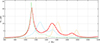 |
Figure 15 Transmission loss for the DNN geometry determined with the direct simulation (“face A” configuration) ( |
The DNN material is now modelled using simultaneously two different equivalent fluids, one corresponding to the small network and the other one to the large network. In this model, the DNN material domain is split into two equal and parallel domains, each containing one of the two equivalent fluids, on either side of the plane y = 0 (see Fig. 16bluea). As in Section 4.2, we consider two boundary conditions at the interface between the two effective fluids. In the configuration called “separated”, a rigid wall separates the two fluids. In the configuration referred to as “contiguous”, the continuity of pressure and normal velocity is enforced at the interface. Figure 16b compares the TL obtained using the direct simulation for the “face A” orientation of the DNN geometry with the TL curve calculated using the multiscale model involving two equivalent fluids. For the “separated” configuration, the TL has two main peaks, that correspond to those of the large and small networks in Figure 15b. However, the value of each peak is largely reduced, as the lined surface associated to each equivalent fluid has been halved. The correspondence with the DNS is thus poor. For the “contiguous” configuration, a single peak is observed; it is located between those associated with the large and small networks. Thus, it is found again that, while the equivalent fluid approach can reproduce some characteristics of the DNN, it cannot accurately predict the TL for this geometry.
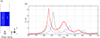 |
Figure 16 (a) Sketch showing the duct and the sample split into two parts, each containing one of the equivalent fluid. (b) Transmission loss for the DNN geometry determined with the direct simulation (“face A” configuration) ( |
5.3.2 Comparison with measurements
Figure 17 compares the TL obtained from the experiments and the direct simulation for the “face A” and “face B” configurations. The TL curves calculated using DNS for “face B” as well as for “face A” have two distinct peaks. Similarly to the normal incidence case, the peaks are closer to each other for “face A” while the frequencies of the peaks are further apart for “face B”. In the experiments, however, we observe a single peak in each measured TL curve. In addition, the TL peak in the measurements appears at a much higher frequency than the first (large) TL peak in the DNS.
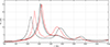 |
Figure 17 Transmission loss for the DNN geometry determined with the direct simulation for the “face A” ( |
Figure 18 focuses on the results obtained for the “face A” configuration. Comparison is performed for the TL obtained from the direct simulation, the experiments and the multiscale approach using two equivalent fluids in the “contiguous” configuration. A good agreement is found between the TL obtained from the experiments and from the equivalent fluid approach. In particular, the frequency of the peak in the experiments is accurately predicted. In the “contiguous” configuration, the acoustic information can transfer from one equivalent fluid to another one, or equivalently from one subnetwork to another. In the DNS, each subnetwork is independent, which explains the difference in the results. The similarity between the TL obtained from the measurements and calculated using two effective fluids in the “contiguous” configuration may indicate that the acoustic waves can somehow propagate between the twosubnetworks.
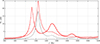 |
Figure 18 Transmission loss for the DNN geometry modelled with two equivalent fluids in the “contiguous” (––) configuration and with the direct simulation for the “face A” ( |
6 Discussion
Although the quality of materials printed from photopolymer resin is good, the manufactured samples still have geometric imperfections and surface irregularities, including roughness mainly related to the thickness of the print layer. In particular, the channels connecting the pores are slightly smaller (see Tab. in appendix) and may be slightly distorted. A perfectly cylindrical shape of the channel was used in the modelling, though with the corrected diameter. These imperfections are to some extent responsible for discrepancies between the experimental results and predictions based on the idealised geometry.
Nevertheless, the agreement between sound absorption predictions by the DNS and JCALP model is very good and agrees well with the measurements (see Fig. 9), especially in the case of single-network materials. The discrepancies between the predictions and experimental results are fully acceptable and typical for 3D printed samples due to printing imperfections. In particular, surface roughness (completely neglected in the modelling) is certainly responsible for the improvement of sound absorption due to the increase of viscous effects. At higher frequencies, i.e. above 2 kHz, the discrepancies can be larger, because the impact of small imperfections is greater, but also due to the poorer scale separation (relatively large pores, only a few periodic cells per layer thickness). It can be expected that better compliance would be achieved for materials with smaller pores and more cells per thickness.
On the other hand, we observed larger discrepancies between the predictions and experimental results in the case of DNN (double nested network), i.e. material with two separate networks. Here, in addition to 3D printing imperfections, the main cause are sound leakages. This is also the case of transmission loss coefficient measured in the duct for 3D printed material as a liner. Acoustic leaks are certainly the cause of the discrepancy between the measured and calculated TL in the case when the OPCL sample or DNN sample were used as liners, see Figures 13 and 17, respectively. However, the TL measured for the cube-pore network material as a liner is in a very good agreement with predictions, see Figure 14. To qualitatively assess the impact of leakage on TL, we carried out measurements with voluntary damages to the Teflon tape around the cubic sample to induce leakage. These measurements show a dramatic effect of the leakage. As an example, for the face A of the cubic sample, few scratches on the Teflon tape can lead to a decrease of the TL peak amplitude by 10 dB and a shift of the peak towards lower frequenciesby 25 Hz.
We believe that better sample sealing is one way to improve the consistency of experimental results and predictions. However, this is not an easy task (although we succeeded in the case of the cubic pore material and in the sound absorption measurements of all materials), because highly tortuous materials (studied in our work) are very sensitive to sound leakages, see reference [3]. Incidentally, we can distinguish two kinds of leakages:
-
leaks through slits around the sample placed in the channel wall (or in the impedance tube);
-
leaks at the back of the sample, i.e. through a very thin layer or air between the sample and the backing wall; in modelling we assumed that it is a perfectly flat and therefore perfectly sealing, rigid wall.
The second kind of leakage is very important in case of double-network material, because it equalises the pressure between two different pore networks that are separated inside the DNN sample. In direct numerical simulation, these networks are fully separated (sealed) also at the back of the material. On the other hand, the “contiguous” configuration of two equivalent fluids seems to grasps this behaviour, see Figure 18.
7 Conclusions
Prediction of the acoustic performance of 3D printed samples was investigated for normal and grazing incidence. We compared the results of a computationally efficient multiscale approach, in which the 3D printed material is represented by an equivalent fluid, with the reference results of the direct microscopic approach, in which the full set of Navier–Stokes equations is solved in the material. Three materials with designed periodic microstructures were examined. These periodic microstructures consist of either a single network of cavities or of a double nested network. The samples were 3D printed using stereolithography to fit into an impedance tube or a duct testing bench. We observe that although the samples contain a small number of periodic unit cells, the equivalent fluid model provides predictions similar to those obtained with the direct microscopic approach for the single network geometries at both normal and grazing incidence. On the other hand, such a single equivalent fluid model is not accurate for the double-nested network geometry, as it fails to predict the effect of the two independent subnetworks. The absorption coefficient measured in the impedance tube is in good agreement with the direct numerical simulations for both geometries. The transmission loss measured in the duct test bench shows a good correspondence with the numerical simulations for single network geometries, although the measured and predicted peak values present noticeable discrepancies. For the double-nested network, the comparison between the transmission loss determined with the direct microscopic approach and from the measurements is rather poor, suggesting that the acoustic information may be transmitted between the two subnetworks in the actual sample.
Acknowledgments
The authors would like to express their gratitude to Jean-Charles Vingiano and Bertrand Houx for their help and their precious advice on additive manufacturing and also to Edouard Salze for additional measurements. This work was supported by the LABEX CeLyA (ANR-10-LABX-0060) of Université de Lyon, within the program “Investissements d’Avenir” (ANR-16-IDEX-0005) operated by the French National Research Agency (ANR). This work was granted access to the HPC resources of PMCS2I (Pôle de Modélisation et de Calcul en Sciences de l’Ingénieur de l’Information) of École Centrale de Lyon, Écully, France. T.G. Zieliński acknowledges the support of Project 2021/41/B/ST8/04492 financed by the National Science Center (NCN), Poland.
Conflicts of interest
The authors declare that they have no conflicts of interest in relation to this article.
Data availability statement
Data are available on request from the authors.
References
- G.D.N. Almeida, E.F. Vergara, L.R. Barbosa, R. Brum: Low-frequency sound absorption of a metamaterial with symmetrical-coiled-up spaces. Applied Acoustics 172 (2021) 107593. [CrossRef] [Google Scholar]
- Y. Wang, H. Zhao, H. Yang, J. Zhong, D. Zhao, Z. Lu, J. Wen: A tunable sound-absorbing metamaterial based on coiled-up space. Journal of Applied Physics 123, 18 (2018) 185109. [CrossRef] [Google Scholar]
- T.G. Zieliński, K.C. Opiela, N. Dauchez, T. Boutin, M.-A. Galland, K. Attenborough: Extremely tortuous sound absorbers with labyrinthine channels in non-porous and microporous solid skeletons. Applied Acoustics 217 (2024) 109816. [CrossRef] [Google Scholar]
- J. Guo, Y. Fang, Z. Jiang, X. Zhang: An investigation on noise attenuation by acoustic liner constructed by Helmholtz resonators with extended necks. Journal of the Acoustical Society of America 149, 1 (2021)70–81. [CrossRef] [PubMed] [Google Scholar]
- M. Duan, C. Yu, Z. Xu, F. Xin, T.J. Lu: Acoustic impedance regulation of Helmholtz resonators for perfect sound absorption via roughened embedded necks. Applied Physics Letters 117, 15 (2020) 151904. [CrossRef] [Google Scholar]
- T. Cavalieri, A. Cebrecos, J.-P. Groby, C. Chaufour, V. Romero-García: Three-dimensional multiresonant lossy sonic crystal for broadband acoustic attenuation: application to train noise reduction. Applied Acoustics 146 (2019) 1–8. [CrossRef] [Google Scholar]
- R. Al Jahdali, Y. Wu: Coupled resonators for sound trapping and absorption. Scientific Reports 8, 1 (2018) 13855. [CrossRef] [PubMed] [Google Scholar]
- T.S. Oh, W. Jeon: Acoustic metaliners for sound insulation in a duct with little flow resistance. Applied Physics Letters 120, 4 (2022) 044103. [CrossRef] [Google Scholar]
- J. Boulvert, G. Gabard, V. Romero-García, J.-P. Groby: Compact resonant systems for perfect and broadband sound absorption in wide waveguides in transmission problems. Scientific Reports 12 (2022) 10013. [CrossRef] [PubMed] [Google Scholar]
- J. Boulvert, T. Humbert, V. Romero-García, G. Gabard, E.R. Fotsing, A. Ross, J. Mardjono, J.-P. Groby: Perfect, broadband, and sub-wavelength absorption with asymmetric absorbers: realization for duct acoustics with 3D printed porous resonators. Journal of Sound and Vibration 523 (2022) 116687. [CrossRef] [Google Scholar]
- Y. Meng, V. Romero-García, G. Gabard, J.-P. Groby, C. Bricault, S. Goudé: Subwavelength broadband perfect absorption for unidimensional open-duct problems. Advanced Materials Technologies 8 (2023) 2201909. [CrossRef] [Google Scholar]
- F. Nistri, V.H. Kamrul, L. Bettini, E. Musso, D. Piciucco, M. Zemello, A.S. Gliozzi, A.O. Krushynska, N. Pugno, L. Sangiuliano, L. Shtrepi, F. Bosia: Efficient broadband sound absorption exploiting rainbow labyrinthine metamaterials. Journal of Physics D: Applied Physics 57, 24 (2024) 245111. [CrossRef] [Google Scholar]
- T.G. Zieliński, K.C. Opiela, P. Pawłowski, N. Dauchez, T. Boutin, J. Kennedy, D. Trimble, H. Rice, B. Van Damme, G. Hannema, R. Wróbel, S. Kim, S. Ghaffari Mosanenzadeh, N.X. Fang, J. Yang, B. Briere de La Hosseraye, M.C.J. Hornikx, E. Salze, M.-A. Galland, R. Boonen, A. Carvalho de Sousa, E. Deckers, M. Gaborit, J.-P. Groby: Reproducibility of sound-absorbing periodic porous materials using additive manufacturing technologies: round robin study. Additive Manufacturing 36 (2020)101564. [CrossRef] [Google Scholar]
- G. Fusaro, L. Barbaresi, M. Cingolani, M. Garai, E. Ida, A. Prato, A. Schiavi: Investigation of the impact of additive manufacturing techniques on the acoustic performance of a coiled-up resonator. Journal of the Acoustical Society of America 153, 5 (2023) 2921–2931. [CrossRef] [PubMed] [Google Scholar]
- A. Ciochon, J. Kennedy, R. Leiba, L. Flanagan, M. Culleton: The impact of surface roughness on an additively manufactured acoustic material: an experimental and numerical investigation. Journal of Sound and Vibration 546 (2023) 117434. [CrossRef] [Google Scholar]
- A. Jamois, D. Dragna, M.-A. Galland: Impact of manufacturing uncertainties on the acoustic properties of 3D printed materials, in: 29th International Congress on Sound and Vibration ICSV29, Prague, Czech Republic. International Institute of Acoustics and Vibration IIAV, 2023. [Google Scholar]
- A. Jamois, D. Dragna, T.G. Zieliński, M.-A. Galland: Modélisation acoustique d’un matériau obtenu par fabrication additive placé en paroi d’un conduit, in: 16ème Congrès Français d’Acoustique, CFA2022, Marseille, France, Apr 2022. [Google Scholar]
- D.L. Johnson, J. Koplik, R. Dashen: Theory of dynamic permeability and tortuosity in fluid-saturated porous media. Journal of Fluid Mechanics 176 (1987) 379–402. [Google Scholar]
- Y. Champoux, Étude expérimentale du comportement acoustique des materiaux poreux à structure rigide. Ph.D. thesis, Carleton University, Canada, 1991. [Google Scholar]
- D. Lafarge, P. Lemarinier, J.F. Allard, V. Tarnow: Dynamic compressibility of air in porous structures at audible frequencies. Journal of the Acoustical Society of America 102, 4 (1997) 1995–2006. [CrossRef] [Google Scholar]
- S.R. Pride, F.D. Morgan, A.F. Gangi: Drag forces of porous-medium acoustics. Physical Review B 47, 9 (1993) 4964–4978. [CrossRef] [PubMed] [Google Scholar]
- J.-L. Auriault, C. Boutin, C. Geindreau: Homogenization of Coupled Phenomena in Heterogenous Media. John Wiley & Sons, 2010. [Google Scholar]
- C. Perrot, F. Chevillotte, R. Panneton: Dynamic viscous permeability of an open-cell aluminum foam: computations versus experiments. Journal of Applied Physics 103, 2 (2008) 024909. [CrossRef] [Google Scholar]
- H. T. Luu, C. Perrot, R. Panneton: Influence of porosity, fiber radius and fiber orientation on the transport and acoustic properties of random fiber structures. Acta Acustica United with Acustica 103, 6 (2017) 1050–1063. [CrossRef] [Google Scholar]
- T.G. Zieliński, R. Venegas, C. Perrot, M. ervenka, F. Chevillotte, K. Attenborough: Benchmarks for microstructure-based modelling of sound absorbing rigid-frame porous media. Journal of Sound and Vibration 483 (2020) 115441. [CrossRef] [Google Scholar]
- L. Jaouen, F. Chevilotte: Length correction of 2D discontinuities or perforations at large wavelengths and for linear acoustics. Acta Acustica United with Acustica 104 (2018) 243–250. [CrossRef] [Google Scholar]
- V.V. Voronina, K.V. Horoshenkov: Acoustic properties of unconsolidated granular mixes. Applied Acoustics 65, 7 (2004) 673–691. [CrossRef] [Google Scholar]
- V. Viet Dung, R. Panneton, R. Gagné: Prediction of effective properties and sound absorption of random close packings of monodisperse spherical particles: multiscale approach. Journal of the Acoustical Society of America 145, 6 (2019) 3606–3624. [CrossRef] [PubMed] [Google Scholar]
- A. Cummings: Impedance tube measurements on porous media: the effects of air-gaps around the sample. Journal of Sound and Vibration 151, 1 (1991) 63–75. [CrossRef] [Google Scholar]
- N. Sellen, M. Cuesta, M.-A. Galland: Noise reduction in a flow duct: implementation of a hybrid passive/active solution. Journal of Sound and Vibration 297, 3–5 (2006) 492–511. [CrossRef] [Google Scholar]
- B. Betgen, M.-A. Galland: A new hybrid active/passive sound absorber with variable surface impedance. Mechanical Systems and Signal Processing 25, 5 (2011) 1715–1726. [CrossRef] [Google Scholar]
- M.L. Munjal: Acoustics of Ducts and Mufflers with Application to Exhaust and Ventilation System Design. John Wiley & Sons, 1987. [Google Scholar]
Appendix A
This appendix reports measurements taken to characterize the dimensions of the unit cells on the samples 3D printed for experiments in the impedance tube and the duct testing bench. The channel and cavity diameters were measured on the surface of the samples, using a Mitutoyo PJ-A3000 profile projector (see Jamois et al. [16] for details). The profile projector has a precision of about a micrometer; however, we restrict the precision to a hundredth of millimeter due to measurement bias. The mean values and standard deviations of the characteristic dimensions are reported in Table A.1. They can be compared to the design values given in Table 1. The dimensions of the cavities are in good agreement with the design values for all samples and the corresponding normalized standard deviation is small, below 2%. The canal diameters tend to be smaller than the design values, especially for normal incidence samples. Furthermore, the normalized standard deviation tends to be higher and reaches 10% to 20% for the DNN small network.
Measured characteristic dimensions of the pore network of samples produced for acoustic characterization at normal and grazing incidence. They are written in the form  , where
  is the mean value and σ is the standard deviation.
Cite this article as: Jamois A. Dragna D. Zieliński T.G. & Galland M.-A. 2025. Acoustic absorption of 3D printed samples at normal incidence and as a duct liner. Acta Acustica, 9, 12. https://doi.org/10.1051/aacus/2024088.
All Tables
JCALP parameters for the OPCL, cubic, and double nested network (DNN) geometries.
Measured characteristic dimensions of the pore network of samples produced for acoustic characterization at normal and grazing incidence. They are written in the form , where is the mean value and σ is the standard deviation.
All Figures
|
Figure 1 (Top) Unit cells for the considered periodic geometries: (a) OPCL, (b) cubic, and (c) DNN. The air-saturated pores are represented in white (and also in blue for the large network of DNN) and the rigid skeleton is in black. (Bottom) Pictures of the corresponding samples 3D printed for testing in a 29 mm impedance tube: (d) OPCL, (e) cubic, (f) DNN. |
| In the text | |
|
Figure 2 Samples for the impedance tube and the duct bench for the geometries OPC (a), cubic (b), and DNN (c). |
| In the text | |
|
Figure 3 Sketch showing the two different faces of the samples. |
| In the text | |
|
Figure 4 Sketch for the DNS of the impedance tube testing. The pressure is averaged on the two surfaces represented by the red lines at the positions of the microphones 1 and 2. |
| In the text | |
|
Figure 5 Absorption coefficient for the OPCL geometry (a) and the cubic geometry (b): results from the equivalent fluid model (——) and from two direct numerical simulations, i.e. for the “face A” (+) and “face B” (+) configurations. |
| In the text | |
|
Figure 6 Sound absorption coefficient α for the hard-backed layer of the OPCL material (red curves) or cubic pore network material (blue curves) versus: (a) frequency f, or (b) 4H/λ w(f) where H is the layer thickness and λ w is the wavelength in the respective equivalent fluid. |
| In the text | |
|
Figure 7 (a) Sketch of the two faces configurations considered for the DNN geometry. (b) Absorption coefficient determined with the direct simulation for the “face A” (+) and “face B” (+) configurations and using the equivalent fluid method with a single equivalent fluid corresponding to the large (--), small (--), or double network (--). |
| In the text | |
|
Figure 8 (a) Sketch of the finite element model for the multiscale approach using two equivalent fluids. (b) Absorption coefficient determined with the direct simulation for the “face A” (+) and “face B” (+) orientations and using the multiscale approach with two equivalent fluids for the “separated” (--) and “contiguous” ( |
| In the text | |
|
Figure 9 Absorption coefficient for geometries OPCL (a) cubic (b), and DNN (c) obtained from the direct simulation for the “face A” (+) and “face B” (+) configurations and from the measurements for the “face A” (—) and “face B” (—) orientations. |
| In the text | |
|
Figure 10 (a) Sketch of the MATISSE bench. (b) Configuration for the numerical simulations for: (top) the DNS and (bottom) for the equivalent fluid approach. |
| In the text | |
|
Figure 11 Transmission loss for the OPCL (a) and cubic (b) geometry: equivalent fluid approach ( |
| In the text | |
|
Figure 12 Map of the acoustic pressure modulus |p|/pind for the OPCL (a) and cubic (b) geometry for the “face A” orientation at the frequency of the TL maximum, (i.e. f = 1240 Hz (a) and f = 980 Hz (b)): direct simulation (top) and equivalent fluid model (bottom). |
| In the text | |
|
Figure 13 Transmission loss for the OPCL geometry modelled with the equivalent fluid approach ( |
| In the text | |
|
Figure 14 Transmission loss for the cubic geometry modelled with the equivalent fluid approach (––) and with the direct numerical simulation for the “face A” ( |
| In the text | |
|
Figure 15 Transmission loss for the DNN geometry determined with the direct simulation (“face A” configuration) ( |
| In the text | |
|
Figure 16 (a) Sketch showing the duct and the sample split into two parts, each containing one of the equivalent fluid. (b) Transmission loss for the DNN geometry determined with the direct simulation (“face A” configuration) ( |
| In the text | |
|
Figure 17 Transmission loss for the DNN geometry determined with the direct simulation for the “face A” ( |
| In the text | |
|
Figure 18 Transmission loss for the DNN geometry modelled with two equivalent fluids in the “contiguous” (––) configuration and with the direct simulation for the “face A” ( |
| In the text | |
Current usage metrics show cumulative count of Article Views (full-text article views including HTML views, PDF and ePub downloads, according to the available data) and Abstracts Views on Vision4Press platform.
Data correspond to usage on the plateform after 2015. The current usage metrics is available 48-96 hours after online publication and is updated daily on week days.
Initial download of the metrics may take a while.