| Issue |
Acta Acust.
Volume 9, 2025
|
|
|---|---|---|
| Article Number | 13 | |
| Number of page(s) | 17 | |
| Section | Musical Acoustics | |
| DOI | https://doi.org/10.1051/aacus/2024089 | |
| Published online | 14 February 2025 | |
Scientific Article
Deriving played trumpet directivity patterns from a multiple-capture transfer-function technique
1
Sorbonne Université, CNRS, Institute Jean le Rond d’Alembert, UMR 7190, 4 Place Jussieu, 75005 Paris, France
2
Acoustics Research Group, Department of Physics and Astronomy, Brigham Young University, Provo, Utah, USA
* Corresponding author: This email address is being protected from spambots. You need JavaScript enabled to view it.
Received:
9
January
2024
Accepted:
9
December
2024
Abstract
The directional radiation patterns of musical instruments have long been defining characteristics known to influence their perceived qualities. Technical understanding of musical instrument directivities is essential for applications such as concert hall design, auralizations, and recording microphone placements. Nonetheless, the difficulties in measuring sound radiation from musician-played instruments at numerous locations over a sphere have severely limited their directivity measurement resolutions compared to standardized loudspeaker resolutions. This work illustrates how a carefully implemented multiple-capture transfer-function method adapts well to played musical instrument directivities and achieves compatible resolutions. Comparisons between a musician-played and artificially excited trumpet attached to a mannikin validate the approach’s effectiveness. The results demonstrate the trumpet’s highly directional characteristics at high frequencies and underscore the crucial effects of musician diffraction. Spherical spectral analysis reveals that standardized resolutions may only be sufficient to produce valid complex-valued directivities up to nearly 4 kHz, emphasizing the need for high-resolution, played musical instrumentdirectivity measurements.
Key words: Trumpet / Directivity / Musical instrument / Sound radiation / Spherical array
© The Author(s), Published by EDP Sciences, 2025
 This is an Open Access article distributed under the terms of the Creative Commons Attribution License (https://creativecommons.org/licenses/by/4.0), which permits unrestricted use, distribution, and reproduction in any medium, provided the original work is properly cited.
1 Introduction
Directional radiation is an essential aspect of played musical instruments. Musical instrument radiation characteristics influence many practical applications, including microphone placements [1–4], auralizations [5, 6], and concert hall designs [7, 8]. Nevertheless, properly acquiring and implementing source directivities for these and other applications requires sufficient spatial resolution. The AES56-2008 (r2019) [9] governs measured spherical directivities for loudspeakers with 5° angular resolution to enable successful electroacoustic and room-acoustical modeling and prediction. Commercially available room acoustical prediction software packages commonly employ these standardized angular resolutions [10, 11]. However, the fine details afforded by comparable resolutions for musical instruments have remained obscure.
Musical instrument directivity measurements present several practical challenges [12]. For example, unlike loudspeakers, musicians cannot repeat notes exactly each time their orientations or scanning microphone positions change, and new measurements begin. Furthermore, while the position of a loudspeaker is easily controllable during a measurement sequence, a musician often shifts while playing. Aligning a principal loudspeaker axis toward desired polar and azimuthal angles is automatable, but practical considerations restrict the rotation of a live musician and their instrument to the horizontal plane (i.e., the azimuthal angle) only.
To evade these and other challenges, some researchers have resorted to artificial excitation of instruments, including horns [13–16], the clarinet [17–19], bassoon[20, 21], violin [18, 22–28], guitar [25, 29], harp [29, 30], and piano [31, 32]. Directivity measurements employing artificial excitation of musical instruments have achieved angular sampling resolutions comparable to the AES standard, such as for the bassoon [21] and trumpet [15, 16]. These finer angular resolutions have revealed salient radiation details that coarser sampling cannot detect, such as numerous side lobes at high frequencies.
While the enhanced repeatability of artificial excitation increases the feasibility of higher-resolution measurements, the approach ignores the critical effects of live musicians, including their diffraction, absorption, and natural instrument excitation. More recently, Bellows and Leishman [19] showed that diffraction and absorption of the human body significantly alter the directivities of isolated instruments, such as the clarinet, even at lower frequencies. Results from Marruffo et al. [16] likewise suggested that the interaction of sound waves with the musician’s body impacts trumpet directivities. Meyer and Wogram correctly stressed that musicians and instruments are intrinsically integrated entities for practical directivity measurements [14]. In fact, while most of Meyer’s published results emanated from artificially excited instruments, he also performed sparse measurements of played instrument directivities in some cases to evaluate the diffraction and absorption caused by musicians’ bodies [14, 20].
One approach to evaluating played musical instruments’ directivities is limiting measurements to individual multichannel recordings. This single-capture method fixes the positions and orientations of musicians and instruments within a stationary enveloping microphone array having limited (e.g., 13, 22, 32, or 64) total sampling positions over the measurement surfaces or contours [5, 33–37]. One of the most significant works to date involving directivity measurements of 41 modern and historical instruments employed a quasi-spherical microphone array with 32 nearly uniformly spaced positions [38].
Single-capture systems do not require playing repetitions and may claim better measurement repeatability. However, the coarse measurement resolutions may lead to spatial aliasing errors at frequencies of interest, limiting the application of measured directional data. For example, radiation from the trumpet and other horns has long been known to be roughly omnidirectional at low frequencies and increasingly directional at higher frequencies, with the strongest radiation in front of the bell [13–16]. Nonetheless, some trumpet directivities interpolated through spherical harmonic expansions appearing in [39] based on the measurements reported in [38] show perplexing patterns, including nulls in front of the bell and strong radiation lobes to the side of the musician. These unplausable directional characteristics suggest that spatial aliasing errors from insufficient sampling resolution may have contaminated the results.
Indeed, the number of spatial sampling positions employed in previous single-capture systems have been significantly fewer than the number recommended by AES56-2008 (r2019) [9]. The 5° angular resolutions specified for standardized loudspeaker directivity measurements would require 2522 unique sampling positions over a sphere, with accompanying microphones, support structures, cables, and data acquisition channels. Because this is an impractical number for single-capture measurements, multiple-capture systems employing moving microphones or sources are necessary to measure played musical instruments, just as they are to measure loudspeakers.
Researchers have previously employed multiple-capture methods in musical instrument directivity studies, such as for the piano [40], violin [41, 42], and traditional Korean musical instruments [8]. However, the works employing the approaches lacked complete spherical data, did not use excitation approaches applicable to all instruments, or did not use actual transfer functions to adequately compensate for differences between playing repetitions necessitated by incremental captures. Recently, two of the present authors published work on a multiple-capture, transfer-function method for measuring live speech directivity with a full-spherical, 5° resolution compatible with the AES standard [43]. Nevertheless, adaptations of multiple-capture methods to musical instruments come with unique challenges and differing results.
This work illustrates how the multiple-capture, transfer-function method adapts to musical instrument directivities by assessing a trumpet’s sound radiation. The applied technique enables 5° polar and azimuthal angular resolution measurements compatible with the AES directivity sampling standard [9]. Narrowband directivities, while confirming well-known general radiation characteristics, reveal intricate radiation patterns, diffraction lobes, and musician shadowing. Comparing results to those of an artificially played trumpet and seated manikin is similar to the approach described in [19] and confirms the reliability of the multiple-capture, transfer-function method. The comparisons also highlight the benefit of directivities derived from played rather than artificially excited musical instruments. Spherical spectral analysis reveals that the sampling resolution is sufficient to produce complex-valued narrowband directivities up to nearly 4 kHz. Derived directivity indices verify that the trumpet is a highly directional source at many frequencies. Additional results and discussions related to source centering and spatial aliasing highlight the benefits of the multiple-capture method in producing high-resolution, spherical directivities. An archival database at [44] provides the directivity results for use by other researchers and practitioners in various acoustics applications.
2 Methods
2.1 Measurement procedure
Several components of the directivity measurement system appear in Figure 1, including a fixed reference microphone, a rotating semicircular microphone array, and a musician and instrument within an anechoic chamber (fc = 80 Hz). The constant-radius R = 1.17 m array incorporated 36 precision free-field 12.7 mm (0.5 in.) microphones at fixed 5° polar-angle increments. Acoustically treated apparatuses suspended and supported the arc and rotation system. The musician’s chair and footrests could adjust vertically, horizontally, and angularly within the rotating arc. References [45, 46] include more details about the measurement hardware and calibration procedures.
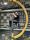 |
Figure 1 Illustration of the directivity measurement system with a musician and Vincent Bach Model 43 Stradivarius B♭ trumpet. The laser pointer was attached to the bottom of the instrument near the water keys. The marked axis indicates the coordinate directions employed in later balloon plots. |
Because the trumpet was not fixed, musician movements could potentially introduce spatial variances affecting the directivity measurement’s quality. To mitigate these variances, a head restraint connected to the musician’s chair and tightened across the musician’s forehead ensured consistent head position within the rotating array. To minimize rotational movements, a laser attached to the instrument (see Fig. 1) illuminated an acoustically unobtrusive ≈2 cm square target fixed to the chamber wall several meters away. The measurement procedure required that the musician hold the trumpet still to align with the target during the playing sequence.
While oriented toward the initial azimuthal angle ϕ = 0°, the musician played a chromatic scale at mezzo-forte from B♭3 to F5, the typical playing range of the instrument, with each note held for 1 s, followed by a 1 s rest. A metronome signal in the musician’s earphone ensured a consistent pace, while an electronic tuner helped maintain pitch consistency. The musician repeated any problematic notes of a scale for correction. Following a successful multichannel recording, the rotation system advanced 5° in the azimuthal angle ϕ, and the musician repeated the scale. This process continued until the directivity measurement system collected a complete sphere of sampled data via 72 multichannel recordings, each with 24-bit, 48 kHz sampling.
As an additional validation, the directivity measurement system evaluated the directivity of the trumpet when it was artificially excited by a small transducer coupled to the trumpet mouthpiece. Three repetitions of a five-second logarithmic swept sine served as the excitation signal. As suggested by Figure 2, the artificial excitation apparatus was attached to a seated manikin. Although the manikin was somewhat smaller, lacked forearms and hands, and otherwise differed in geometry, it provided a rough approximation of the diffraction and absorption caused by the musician’s body [16, 19]. A support structure aligned the instrument and its laser to the same target on the anechoic chamber wall.
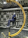 |
Figure 2 Illustration of the directivity measurement system with an artificially excited trumpet and manikin. |
2.2 Data processing and analysis
2.2.1 Narrowband
Because even the best musicians play repeated notes with amplitude and spectral variations, imperfect repetitions seemingly pose an insurmountable problem for multiple-capture directivity measurements. However, when appropriately employed, frequency response functions (FRFs) between the reference and array microphone signals mitigate these effects. Previous research has demonstrated that FRFs establish directivity functions for loudspeakers [47], the human voice [43, 48], and musical instruments [42, 49]. However, for musical instruments playing discrete notes (i.e., without glissandi), the FRFs must derive from spectrally sparse signals and are valid only at specific frequencies for which significant radiated sound energy arrives at both the reference and array microphones.
The FRFs for the uth microphone at the vth azimuthal rotation followed from the autospectral estimates Gaav(f) of the reference microphone signal av(t) and the cross-spectral estimates  between that signal and each array microphone signal
  , where the tilde indicates the possibility of uncorrelated noise in the array signals. For each note, the spectral estimates resulted from Welch’s method [50, 51] and involved five 48 000-sample block sizes (1 s record length, 1 Hz narrow-band resolution), a Hann window, and 90% overlap. For each reference and array microphone pair, the FRF estimate
 (1)
(1)
provided an unbiased result with respect to uncorrelated noise in the output signals [51]. A normalized FRF-based directivity function follows as [43]
 (2)
(2)
where (u v)max|H| represents the index pair with the maximum FRF magnitude for a given frequency.
2.2.2 Spherical harmonic expansions
Spherical harmonic expansions provide several benefits to directional data discretely sampled over the sphere. First, the expansions provide a continuous representation of the pressure field for further interpolation. Second, spherical harmonic expansions applied to complex-valued narrowband pressure data allow extrapolation of far-field directivity functions [46, 52]. Third, the spectrum of the expansion provides essential information on spatial aliasing and establishing viable frequency ranges for directivities [53]. Fourth, truncation of spherical harmonic expansions may be leveraged for spatial filtering.
A spherical harmonic expansion applied to complex-valued narrowband data yields the unique solution on the exterior domain [54]:
 (3)
(3)
where  is the complex pressure amplitude, r is the radial distance from the origin, R is the measurement sphere radius, k is the wavenumber, hn(2)(kr) are the spherical Hankel functions of the second kind of order n (for outward-going waves with eiωt time dependence), Ynm are the spherical harmonics of degree n and order m [55], and pnm(k) are the pressure expansion coefficients. The expansion coefficients follow from orthogonality as
![Mathematical equation: $$ \begin{aligned} p_n^m(k) = \int _0^{2\pi }\int _0^\pi \hat{p}(R,\theta ,\phi ,k) \left[Y_n^m(\theta ,\phi )\right]^*\sin \theta \,\mathrm{d}\theta \,\mathrm{d}\phi , \end{aligned} $$](/articles/aacus/full_html/2025/01/aacus240005/aacus240005-eq7.gif) (4)
(4)
where * indicates complex conjugation. A normalized continuous directivity function on the measurement surface follows as [43]
![Mathematical equation: $$ \begin{aligned} D(R, \theta ,\phi ,k) = \frac{\hat{p}(R,\theta ,\phi ,k)}{\hat{p}[R, (\theta ,\phi )_{\text{ max}|\hat{p}|},k]}\cdot \end{aligned} $$](/articles/aacus/full_html/2025/01/aacus240005/aacus240005-eq8.gif) (5)
(5)
A sound source’s directivity varies over increasing radial distance r until converging to a radially independent far-field directivity function [56]. However, practical constraints, such as anechoic chamber size, often limit the array sampling radius so that measurements may not always fall in the source’s far field. For example, the acoustic far field requires that kR ≫ 1 while the geometric far field requires that R ≫ Rs, where Rs is the dimension of the source [56]. For the present work, the R = 1.17 m array suggests that while frequencies above 500 Hz may be in the acoustic far field, the large size of the musician relative to the array radius (see Fig. 1) does not satisfy the geometric far-field constraint. Consequently, the measurements should not be assumed to be in the source’s far field.
Differences between measured directivity patterns in the near field of a source and the oft-desired far-field pattern have motivated the use of acoustic centering algorithms [38, 39, 57, 58]. These methods generally attempt to expand the pressure field about a source’s acoustic center so that the near-field measurements are “representative of farfield performance" [59, 60]. However, rather than attempting to modify near-field results, one may directly obtain an unnormalized far-field directivity by propagating the measured pressure with r → ∞ as [46, 53, 56]:
 (6)
(6)
which follows from the large-argument approximation of the spherical Hankel functions valid for r ≫ kR. Interestingly, the magnitude of this far-field directivity is independent of source location within the array [52, 61]. Source translation does modify the far-field directivity’s phase according to [52, 61]
 (7)
(7)
where  is the unit vector in the direction of r, rt is the translation vector, and Dff, t is the far-field directivity after translation. Once one determines the acoustic center rc, setting rt = −rc in equation (7) provides a far-field phase correction by virtually moving the source back to the acoustic center (see Sect. 3.4 and [62]).
Some computational techniques, such as geometric or ray-based methods, only employ magnitude far-field values [63]. In these cases, equation (6) suffices for practical applications of directional data. Some have also considered the relevance of phase data for interacting coherent sources [64], in which case the phase simplification afforded by acoustic centering may also be beneficial. In wave-based simulations using complex-valued narrowband data [65, 66], the expansion of equation (3) provides the unique solution on the exterior domain r > R [54]. Consequently, acoustic source centering is not necessary to obtain the correct solution. Nonetheless, acoustic centering may benefit computational efficiency by reducing the number of necessary expansion coefficients [39, 57].
The far-field directivity factor function follows from the far-field directivity function as [56]
 (8)
(8)
For comparisons between two directivities, a directivity factor function deviation follows as [46]
 (9)
(9)
It may be expressed as a directivity factor function deviation level as
 (10)
(10)
where the addition of 1 in the argument of the logarithm maps σQ = 0 to 0 dB. Importantly, this metric may be used to monitor the convergence of spherical harmonic expansions over increasing expansion degree (see Sect. 3.2).
2.3 Source order and spatial aliasing analysis
The discrete spherical sampling employed in directivity measurements limits computation of the expansion coefficients pnm to maximum degree Nd, effectively truncating the infinite series in equation (3). This maximum expansion degree depends on the number of sampling positions, their distribution over the sampling sphere, and is independent of source characteristics [67]. The 5° dual equiangular sampling scheme allows expansions to Nd = 34 [68] when using spherical quadrature weights [69] to numerically evaluate the orthogonality integral in equation (4).
The proper application of spherical harmonic expansions, including the far-field propagation of equation (6), requires that the maximum spherical harmonic expansion degree necessary to represent the source Ns be less than or equal to that resolvable by the sampling array Nd. Otherwise, spatial aliasing occurs, meaning that errors appear in calculated values of pnm and the spherical-harmonic-based representation becomes invalid [67, 68]. Consequently, estimating Ns is essential to establishing usable frequency ranges for directivity validity and analysis.
For a source enclosed by a notional sphere of radius Rs centered at the origin, the evanescent nature of the spherical Hankel functions suggests that the relative contributions of the expansion coefficients with n ⪆ kRs decrease rapidly in the far-field [54, 67, 70]. As a result, a sound source with “effective radius” [70] Rs requires an expansion with terms up to roughly Ns ≈ kRs [53]. This simple relationship suggests that a source is spatially band-limited so that one may effectively truncate the infinite series in equations (3) and (6) at a frequency dependent Ns without significant errors. Because spatial aliasing occurs when Ns exceeds Nd, this relationship also implies that the maximum usable wavenumber for analysis of complex-valued directivities is
 (11)
(11)
This equation highlights that for a fixed source extent, the only way to increase the viable frequency bandwidth for analysis is increasing the sampling resolution to increase Nd. Additionally, because Rs is the spatial extent of the source as measured from the origin, poor source placement may cause Rs to be much larger than the source’s actual dimensions [61].
Estimating Rs from measured data is essential to deduce the maximal usable frequency for spherical-harmonic-based analysis without spatial aliasing errors. The energy-per-degree metric [71]
 (12)
(12)
serves as a useful tool for this purpose. It represents the spatial signal energy for a specified expansion degree n summed over all orders m and provides a measure of a source’s spherical spectrum. Since a source with effective radius Rs radiates little energy to the far field for n > kRs, the ratio
 (13)
(13)
represents the spatial signal energy lost by the infinite series truncation to degree N. In practice, a finite summation up to N d replaces the infinite summation in the denominator. For a fixed threshold, e.g., γ = 0.98, computing N for several discrete wavenumber k values allows a least-squares fit to the line N = kRs as
 (14)
(14)
where the index j references the set of sampled wavenumbers and Nj(0.98) is the minimum N which satisfies γ(N, kj)=0.98. To ensure spatial aliasing effects do not negatively impact the estimate, the maximum wavenumber considered in the least-squares fit should be no more than Nd/R, which corresponds to 1.6 kHz for the present work. This limit represents the maximum frequency for spherical-harmonic-based analysis applied to an arbitrarily-shaped source entirely contained within the measurement radius R. Of course, higher-frequency analysis is possible for sources with effective radii Rs < R.
Besides establishing a valid frequency range for complex-valued narrowband data, the concept of an effect radius is beneficial for post-processing directivity patterns. Truncations of spherical harmonic expansions smooth directivity patterns, enabling spatial filtering to reduce measurement noise [54]. Because the essential expansion coefficients and radiated energy tend to lie along and below n = kRs, coefficients higher than this limit are prone to a lower signal-to-noise ratio, assuming Gaussian spatial noise. Truncation of these higher-degree coefficients according to
 (15)
(15)
thus allows appropriate spatial filtering of the measured data [54]. In equation (15), the ceiling function ⌈ ⌉ rounds up to the nearest integer and the arbitrary addition of two helps preserve energy from the roll-off above n = kRs (see Sect. 3.2).
3 Results
3.1 Narrowband frequency response functions
Playing inconsistencies between repeated captures can lead to significant level deviations in the array microphone signals. Figure 3 highlights the effectiveness of the FRF method in compensating for these variations by comparing narrowband (1 Hz resolution) normalized directivity functions derived from the array autospectral levels (Fig. 3a) with those derived from FRFs (Eq. (2) and Fig. 3b) for the 3rd partial of B♭ (699 Hz). Balloon colors and radii indicate relative levels on a decibel scale. The musician faces the 0° azimuthal marker, and the vantage point is upward and to the musician’s right.
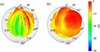 |
Figure 3 Trumpet narrowband directivities at 699 Hz based on (a) autospectral levels from the uncalibrated array microphone signals and (b) calibrated frequency-response functions between the reference and array microphone signals. |
As one might anticipate, the first directivity pattern is hardly discernible without adequate normalizations for playing repetitions and their associated captures at the azimuthal angle increments. The fixed reference microphone data indicated that level variations for this specific partial and frequency exceeded 30 dB, which may be due to both playing level and slight frequency shifts. The input-level variations led to the strong longitudinal banding artifacts in the output measured by the array.
On the other hand, the FRFs between the reference and array microphone signals are robust to these variations, assuming that the pertinent sound propagation mechanisms comprise an LTI system. As evidenced by the FRF-based balloon in Figure 3b, the FRFs compensated for these deviations, leading to a smooth directivity function with no visible banding effects. This typical result highlights the effectiveness of the transfer-function method for narrow bands (and broader bands) when properly applied to radiation from played musical instruments.
Another essential validation of the FRF method follows by comparing directivities produced by the played and artificially excited trumpet. Figure 4 plots narrowband (1 Hz resolution) FRF-based directivity balloons (Eq. (2)) for four different partials from the played trumpet (Figs. 4a–4d) and the equivalent extracted frequencies for the artificially excited trumpet (Figs. 4e–4g). The selected frequencies followed from extracting peaks of the effective input autospectrum [43] for a given note. The vantage point is upward and primarily to the musician’s right side. At 233 Hz (B♭3, 1st partial, Figs. 4a and 4e), the radiation at the array surface is not particularly directional, although some diffraction and shadowing behind the musician appear. At 311 Hz (E♭4, 1st partial, Figs. 4b and 4f), stronger radiation in front of the musician and a side lobe become apparent. Shadowing attenuation behind the musician exceeds 10 dB. These trends continue to develop at 438 Hz (A4, 1st partial, Figs. 4c and 4g), and 524 Hz (C4, 2nd partial, Figs. 4d and 4h). At these frequencies, the strongest radiation regions concentrate in front of the trumpet, and reduced levels appear behind and in the directions of the musicians’ legs. Similar diffraction features are visible in speech and clarinet directivity measurements [19, 43].
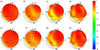 |
Figure 4 FRF-based directivity balloons for the (a)–(d) played and (e)–(h) artificially excited trumpet with manikin. (a) and (e): 233 Hz. (b) and (f): 311 Hz. (c) and (g): 438 Hz (d) and (h): 524 Hz. |
Despite the inherent differences between a musician and a manikin, the directivities derived from the played trumpet qualitatively agree with those derived from the artificially excited trumpet. Although some lobes’ precise directions and locations show minor variations, the essential directional characteristics, including the numbers of lobes and regions of reducedlevels, concur. The LQ between the played and artificially excited directivities did not exceed 1.0 dB for these partials. The individual LQ were 0.7 dB, 0.8 dB, 1.0 dB, and 1.0 dB for 233 Hz, 311 Hz, 438 Hz, and 524 Hz, respectively. These similarities and the absence of longitudinal banding highlight the FRF method’s robustness in compensating between repeated measurements and deriving high-resolution directivities of played musical instruments.
Figure 5 plots the directivity balloons of four higher-frequency partials for the played trumpet (Figs. 5a–5d) and the equivalent extracted frequencies for the artificially excited trumpet (Figs. 5e–5g). The vantage point is upward and behind the musician and manikin to facilitate visualization of the diffraction and interference patterns around and behind the bodies. At 589 Hz (D4, 2nd partial, Figs. 5a and 5e), the most substantial radiation concentrates directly in front of the musician, and two side lobes and a diffraction spot appear behind the musician’s chair. Increased diffraction effects behind the body and complex regions of constructive and destructive interference characterize the directivity patterns at this higher frequencies, especially at 1160 Hz (B♭3, 5th partial, Figs. 5d and 5h). These detailed diffraction and interference patterns require higher sampling resolutions afforded by the multiple-capturemethod.
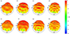 |
Figure 5 FRF-based directivity balloons for the (a)–(d) played trumpet and (e)–(h) artificially excited trumpet with a manikin. (a) and (e): 589 Hz. (b) and (f): 737 Hz. (c) and (g): 932 Hz (d) and (h): 1160 Hz. |
The qualitative agreement continues between the general radiation characteristics of the played and artificially excited trumpets at these higher frequencies. However, some finer details appear to differ, potentially due to the inherent differences between the musician and the manikin. The LQ were 1.2 dB, 1.5 dB, 1.6 dB, and 1.5 dB for 589 Hz, 737 Hz, 932 Hz, and 1160 Hz, respectively. Section 4.2 further considers deviations between played and artificially excited directivities.
3.2 Spherical harmonic expansions
Spherical harmonic expansions are beneficial for directivity interpolation, far-field propagation, and other processing applications. However, their implementation requires careful convergence analysis to ensure adequate expansion terms. Figure 6 plots the directivities derived from spherical harmonic expansions of the complex-valued FRFs over varying expansion degrees evaluated on the measurement surface r = R (Eq. (5)) for the second partial of F4 (695 Hz). The expansions limited to N = 3 (Fig. 6a) or N = 4 (Fig. 6b) are insufficient to capture the general radiation trends at this particular frequency. The LQ between the raw FRF-based directivity (Fig. 6f) and each of these expansion directivities are 4.4 dB and 3.9 dB, respectively. An N = 6 expansion (Fig. 6c) produces general directional characteristics that begin to resemble the original measured data and decreases the LQ to only 1.3 dB. The N = 8 (Fig. 6d) and N = 12 (Fig. 6e) expansions further decrease the LQ to 0.4 dB and 0.2 dB,respectively.
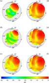 |
Figure 6 Played trumpet directivities at 695 Hz (F4, 2nd partial) based on (a) N = 3, (b) N = 4, (c) N = 6, (d) N = 8, and (e) N = 12 degree spherical harmonic expansions, and (f) the raw FRF-based directivity. |
The number of required expansion coefficients depends on the directivity pattern’s complexity, which typically increases with frequency. To highlight this concept, Figure 7 plots LQ between the original measured data and the expanded data for varying maximal expansion degree N and four partials. For the 233 Hz case (B♭3, 1st partial) shown by the solid red curve, the deviation levels decrease to below 1.0 dB with only an N = 3 degree expansion. However, for the 1315 Hz case (E4, 4th partial) shown by the purple dotted curve, the levels do not reach this same threshold until an N = 13 degree expansion. Thus, properly implementing spherical harmonic expansions requires careful monitoring of both frequency-dependent effects and convergence to measured patterns.
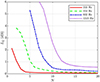 |
Figure 7 Directivity factor function deviation levels between measured FRF-based and spherical-harmonic-expansion-based directivities over expansion degree N for selected partials. |
Considering a source’s effective radius provides additional insight into the increasing number of expansion terms required with increasing frequency. Figure 8 plots the energy per degree En over frequency and expansion degree (see Eq. (12)) for the played (Fig. 8a) and artificially excited (Fig. 8b) trumpet. Color indicates the relative level on a decibel scale, with white representing expansion coefficients with high levels and black representing expansion coefficients with low levels.
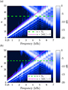 |
Figure 8 Spherical spectrum (E n ) for the (a) played and (b) artificially excited trumpet. |
With a truncation factor of γ = 0.98 (see Sect. 2.2.2), least-squares fits estimated the effective radius of the played trumpet and musician and the artificially excited trumpet with manikin to be Rs = 0.44 m and Rs = 0.45 m, respectively. Overlaid magenta dotted lines in Figures 8a and 8b indicate the truncation curve N = ⌈kRs⌉+2 that uses these values. Below 3 kHz, most of the significant coefficients lie below this line. The essentialexpansion coefficients, indicated by the white streaks, follow the trend of n = kRs.
The overlaid green dashed line represents the upper expansion degree without significant spatial aliasing, Nd = 34 [68]. Near 4.5 kHz, significant signal energy reflects across this line, which is analogous to time-frequency domain aliasing, where the frequency f = fs/2 + Δf aliases to f = fs/2 − Δf, where fs is the sampling rate. Accordingly, the reflected energy in the plot is a key indicator of the reliable bandwidth without spatial aliasing [68]. Using the intersection of N = ⌈kRs⌉+2 with Nd = 34 yields an upper usable limit of 3.9 kHz. Above this frequency, spatial aliasing effects are significant and pressure field extrapolation or interpolation using spherical harmonic expansions may be unreliable.
With an estimate of the effective source radius in place, appropriately truncating the spherical harmonic expansion enables spatial filtering, which can remove undesirable measurement noise [54]. To illustrate this concept, Figure 9a plots a raw FRF-based directivity balloon for the fourth partial of E4 (1315) Hz. Although the compensation by the FRF method is substantial compared, for example, to the directivity of Figure 3a, minor longitudinal banding remains due to measurement inconsistencies between repeated captures. For this particular frequency, equation (15) with an effective radius of Rs = 0.44 suggests that a truncation at N = 13 will maintain the essential directional characteristics while eliminating measurement noise contained in higher-degree expansion coefficients and smoothing the residual banding. Figure 9b plots the resultant directivity expanded to this degree. The LQ between the FRF-based and smoothed result was 0.8 dB.
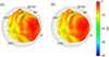 |
Figure 9 Directivity at 1315 Hz (E4 4th partial) based on (a) raw narrowband FRFs and (b) an N = 13 degree spherical harmonic expansion. |
3.3 Far-field propagation
Far-field propagation via spherical harmonic expansions yields the unique far-field magnitude pattern independent of source positioning within the array [52, 61]. Figure 10 illustrates how far-field propagation may modify measured directivities for three selected partials. Figure 10a shows the played trumpet directivity at 394 Hz (G4, 1st partial) while Figure 10d shows its far-field projected pattern using an N = 6 degree expansion. The directional characteristics remain similar, but the radiated levels are stronger to the side and behind. Because the trumpet bell lies in front of (+x) and above (+z) the array’s geometric center (see Fig. 1), the source placement suggests that the near-field directivity will have stronger levels directly in front of the bell than the far-field directivity, as is the case for a displaced monopole [52]. Similar changes are visible in Figures 10b and 10e, which compare the directivities at 986 Hz (E4, 3rd partial) with an N = 10 degree expansion.
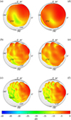 |
Figure 10 Directivity balloons based on (a)–(c) raw narrowband FRFs and (d)–(f) far-field propagated spherical harmonic expansions. (a) and (d): 394 Hz. (b) and (e): 986 Hz . (c) and (f): 1558 Hz. |
Figure 10c shows the measured directivity at 1558 Hz (C5, 3rd partial). At this higher frequency, one may anticipate that the principal radiation axis will be in front of the musician, where body diffraction effects impact radiation less significantly [72]. However, the measured pattern indicates that the principal axis falls slightly above the direction of the bell at an elevation angle of approximately 25° (polar angle θ = 65 ° ). In contrast, the far-field projected directivity shown in Figure 10f with an N = 15 degree expansion lowers the principal axis to an elevation angle of about 15° (θ = 75 ° ).
3.4 Acoustic centering
Although the far-field directivity function of equation (6) is suitable for both geometric and wave-based simulations, acoustic centering may reduce the complexity of the phase pattern and may reduce Ns. The low-frequency acoustic center [60] applied to the lowest note (B♭3, 233 Hz, kRs ≈ 2.0) identified the acoustic center of the source at rc = (0.22, 0.01, 0.47) m, which roughly corresponds to the location of the instrument’s bell (compare Fig. 1).
3.5 Directivity index
The directivity index (DI) has been a fundamental metric of source directivity for decades. Although one may calculate the DI and its associated directivity factor in any direction [56], most authors report it referenced to a source’s principal radiation axis only. This axis is clear for many sources, such as typical loudspeakers and horns. However, it is unrealistic for other more complicated sources, including many played musical instruments. Some sources are multidirectional [46, 47]. Others have complex interference and diffraction patterns. Some, like the human voice, have maximum radiation directions that vary with frequency [46, 73]. The trumpet likewise exhibits an angularly varying maximum radiation direction, although the instrument’s bell may be considered the principal radiation axis.
Figure 11a plots the frequency-dependent DIs of the played and artificially excited trumpet derived from the far-field directivity pattern. Figure 11b presents the frequency-dependent elevation angle for the maximum radiation axis over the sphere. The markers represent 171 extracted partials from the first ten harmonics of the twenty played notes (29 partials lie above the 4 kHz spatial aliasing limit). The far-field corrections produce calculated DIs of about 1.5 dB at the lowest frequencies. The DIs slowly increase to about 5 dB at 1 kHz. Above 1 kHz, they increase by about 2 dB per octave until approaching approximately 15 dB at 4 kHz.
 |
Figure 11 Frequency-dependent trumpet directivity properties: (a) Directivity index and (b) maximum radiation axis elevation. |
Below 1 kHz, the elevation angle of the direction of maximum radiation fluctuates widely. However, above 1 kHz, the variability narrows until the values converge to near −5° at the highest frequencies, corresponding to the direction of the instrument’s bell. These results suggest that at low frequencies, wave effects such as diffraction about the human body influence the maximum direction of radiation. However, at higher frequencies, this direction corresponds to the specular radiation from the bell.
4 Analysis
4.1 Zenith variance
The FRF method employed in this work operates under the assumption that the trumpet’s sound radiation behaves as an LTI system. Because the zenith (north pole) microphone should remain at the same place relative to the trumpet during the array rotation, the variance of this microphone’s directivity level provides insights into FRF variability and repeatability between the 72 repeated captures. Indeed, the AES56-2008 (r2019) directivity sampling standard specifies that the pole positions may be used to validate directivity measurement repeatability, although it does not provide a metric to do so [9]. The present work applies a zenith directivity factor function deviation level LQ, z to quantify the variability as
 (16)
(16)
where
![Mathematical equation: $$ \begin{aligned} \sigma _{{Q,z}} = \frac{\left[\sum _{v = 0}^{V-1} |Q_{0v}(f) - \langle Q_{0v}(f)\rangle _v|^2\right]^{1/2} }{\langle Q_{0v}(f)\rangle _v}, \end{aligned} $$](/articles/aacus/full_html/2025/01/aacus240005/aacus240005-eq21.gif) (17)
(17)
Q0v is the directivity factor function (Eq. (8) but with Dff(θ, ϕ, f) replaced with Duv(f)) at the zenith sampling position (u = 0), and ⟨Q0v(f)⟩v is its azimuthally averaged value.
Figure 12 plots L Q, z for two hundred extracted partials from both the musician and manikin-based directivities. Solid curves represent the average deviations over 1/3-octave bands to help visualize the frequency-dependent trends better. The deviations remain small up to 1 kHz; LQ, z does not exceed 0.6 dB for the played instrument and 0.3 dB for the artificially excited instrument. Above 1 kHz, the deviations begin to increase, and at 4 kHz, they are consistently above 1.0 dB. However, the deviations for all played partials remain below 2.5 dB. The variability of the measurements made with artificial excitation tend to be lower than those produced by the musician except at the highest frequencies. The average level over all frequencies is 0.8 dB for the musician and manikin. These results quantify the repeatability of the FRF-based method in compensating for varying repetition levels with restrained musician movements.
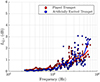 |
Figure 12 Directivity factor function deviations at the zenith microphone position between the 72 repeated captures. |
4.2 Comparison with artificially excited directivity
The artificially excited trumpet provides meaningful validation of the FRF-based multiple capture method and its high-resolution directivity measurements. Figure 13 plots LQ for the same two hundred partials to quantify deviations between the played and artificially excited directivity measurements. The levels follow from the raw FRF-based measurements with no spherical harmonic expansion or other post-processing applied. The red curve shows the 1/3-octave-band averages and better illustrates the general trends. For the lowest frequencies considered, the deviations remain below 1.0 dB. As frequency increases, they slowly rise to about 2.0 dB at 2 kHz. The deviations vary more significantly near and above 2 kHz, with some levels exceeding 3.0 dB and others dropping below 2.0 dB. The general frequency-dependent trend increases with increasing frequency. The average LQ across all partials is 2.1 dB.
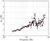 |
Figure 13 Directivity factor function deviation levels between the played and artificially excited FRF-based directivity results. |
The relatively low LQ over frequency highlights the repeatability of the FRF method. The increase of LQ with frequency does not necessarily suggest that the FRF method is becoming less valid; it may merely indicate that geometric and material differences between the musician and manikin lead to increased deviations at higher frequencies. For example, the directivities at 1160 Hz seen in Figures 5d and 5h do not show any severe longitudinal banding in the FRF-based measurements; the reported deviations in Section 3.1 of around 1.5 dB appear to result from variations in the locations of diffraction lobes and attenuation regions around the musician. Indeed, LQ, z at this frequency is only 0.4 dB, indicating high FRF repeatability. Nonetheless, while the pole variance may be a better indicator of measurement reliability, the relatively low LQ between the played and artificially excited directivities over frequency provides an essential validation of the multiple-capture method.
4.3 Symmetry
For many sources, symmetry is another key indicator of directivity validity, such as the quasi-symmetry about the median plane for speech [43]. From geometrical arguments, one would also expect quasi-symmetry about the median plane for the trumpet, especially at lower frequencies. The equiangular sampling scheme employed in the present work facilitates symmetrizing about the median plane. The process involves averaging data from opposing points on the measurement sphere so that the symmetrized directivity factor function becomes
![Mathematical equation: $$ \begin{aligned} Q_s(\theta ,\phi ,f) = \frac{1}{2}\left[Q(\theta ,\phi ,f) + Q(\theta ,-\phi ,f)\right], \end{aligned} $$](/articles/aacus/full_html/2025/01/aacus240005/aacus240005-eq22.gif) (18)
(18)
where Q is the original function and Q s is the symmetrized function. If a source exhibits high symmetry, deviations between the measured Q and symmetrized Qs should be slight. A symmetrized directivity factor function deviation level LQ, s quantifies these variations by calculating LQ (Eq. (9)) between Q and Qs.
Figure 14 plots LQ, s between the measured and symmetrized data for the played and artificially excited trumpet. The symmetry levels in both cases are nearly the same below 1 kHz and consistently fall below 0.6 dB. As frequency increases, LQ, s and their differences tend to increase. However, the frequency averaged values are 0.9 dB and 1.0 dB for the played and artificially excited trumpet, respectively, indicating high symmetry.
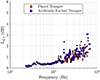 |
Figure 14 Directivity factor function deviation levels between measured and symmetrized partials for played and artificially excited trumpet. |
4.4 Comparison of results from previous work
The multiple-capture method developed in this work allows significantly higher sampling resolutions for played musical instruments than in previous works. Higher sampling resolutions are beneficial to resolve finer radiation details and essential to avoid spatial aliasing effects due to undersampling. As suggested by Section 2.3, one of the primary advantages of high-resolution directional data is that it allows the application of directional data to higher frequencies necessary for realistic acoustic simulations. The effective source radius estimate of Rs = 0.44 m, use of Nd = 34 expansions, and the spherical spectra plots of Figure 8 suggest that the 5° dual equiangular sampling scheme provides sufficient spatial sampling to produce trumpet directivities up to around 4 kHz.
In contrast, previous research employing single-capture methods do not achieve comparable validity ranges. For example, the more recent work of Weinzierl et al. [74] contains musical instrument directivities for a played trumpet using a R = 2.1 m, 32-point measurement scheme capable of Nd = 4 spherical harmonic expansions. Although the source placement and musician size differ between studies, an initial rough estimate using the same effective source radius of Rs = 0.44 m suggests that complex-valued narrowband directivities may only be valid to around 500 Hz (slightly above B4). Because the played notes in this work ranged from B♭3 (233 Hz) to F5 (698 Hz), a comparable 32-point sampling cannot represent the complex-valued pressure for many of these note’s fundamental frequencies and their associated partials.
To consider the viable frequency range for such coarse spatial resolutions, Figure 15 plots the spherical spectrum based on processed trumpet directivities from the original recordings available from [74]. The overlaid dotted magenta line indicating n = kRs with Rs = 0.44 m (see Fig. 8) appears to be in reasonably good agreement with the strongest band of signal energy despite differences between the two works. The spectrum reveals that only the lowest partials below 300 Hz exhibit a band-pass nature, suggesting that spatial aliasing likely occurs near or below 500 Hz.
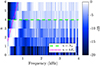 |
Figure 15 Spherical spectrum (E n ) for the trumpet directivity measurements available in [74] based on 32 sampling positions. |
To consider how spatial aliasing effects impact directivities, Figure 16 compares played trumpet directivity results derived from the original recordings from [74] with those of present work for selected partials. Figures 16a–16d plots far-field directivities from the present work over the 5° degree, 2521-point sampling scheme expanded according to equation (15), Figures 16e–16h plots directivities from Weinzierl et al. over the original 32 sampling positions, and Figures 16i–16l plots directivities from Weinzierl et al. interpolated via spherical harmonic expansions to the same sampling position as the present work. All directivity balloon plots employ linear interpolations between sampling positions to better visualize the location of the discrete sampling positions.
 |
Figure 16 (a)–(d) Far-field projected directivity balloons from the present work. (e)–(h) Played trumpet directivity balloons derived from recordings available from Weinzierl et al. [74] plotted over the original 32 sampling positions and (i)–(l) interpolated via an N = 4 spherical harmonic expansion to the same 2521 sampling positions as the present work. (a), (e), and (i): 277 Hz (D♭4). (b), (f), and (j): 738 Hz (G♭5). (c), (g), and (k): 1314 Hz (E6). (d), (h), and (l): 1869 Hz (B♭6). |
Comparisons between the original sampling positions from both works (Figs. 16a–16d and 16e–16h) show similar directional features, including increasing directionality with increasing frequency and similar general diffraction and shadowing effects by the musician. Nonetheless, the higher-resolution measurements provide significantly more detail and additional insights into the finer source radiation and diffraction features. For example, the low-resolution measurements fail to detect minor side lobes, a feature noted in the high-resolution, 0.5° polar measurements of an artificially excited trumpet performed by Marruffo et al. [15].
While the directivity interpolated via spherical harmonics shows reasonable agreement with the corresponding result from the present work for the fundamental of D♭4 (Figs. 16a and 16i), the higher notes, which all fall above 500 Hz, show significant deviations. The LQ between the four partials are 1.2 dB, 2.2 dB, 3.1 dB, and 3.1 dB. Additionally, the directivities in Figures 16j though 16l show strong asymmetries similar to those appearing in [39]. These include non-physical radiation from the musician’s side (see Fig. 8 of [39]).
In that work, the authors noted that the acoustic centering algorithm “achieves good results in the range of up to 400 Hz," [39] which corresponds well to the spatial aliasing limitations suggested by Figure 15. Indeed, Deboy [57] found converging results beyond 1 kHz for a similar centering algorithm applied to a trombone measured by a system allowing Nd = 7 expansions (see Fig. 7.46 of [57]). Thus, the algorithm’s failure to converge in [39] likely resulted from spatial aliasing effects above 400 Hz rather than limitations of the algorithm itself. Asymmetries, spurious and non-physical radiation lobes, and deviations from measured high-resolution results above 500 Hz strongly suggest that insufficient sampling resolution has led to deleterious spatial aliasing.
Figure 17 compares the frequency-dependent maximum DI values derived from Weinzierl et al. [74] with those of the present work for played trumpets. Both works show similar DI increases from around 2.5 dB at 250 Hz to 5 dB by 1 kHz and more than 10 dB by 3 kHz. More significant discrepancies arise above 3 kHz, but it is important to note that a 32-point measurement array can at most evaluate a DI of 10log10(32)≈15 dB, [75] meaning the DI values near that level are less reliable. Additionally, insufficient sampling may further degrade estimates of the source’s DI. Frequency-averaged deviations between the two data sets were less than 1.0 dB below 1 kHz but rose to 3.9 dB when considering all values below 4 kHz.
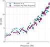 |
Figure 17 Played trumpet directivity indices from Weinzierl et al. and the present work. |
5 Discussion
The multiple-capture method provides a feasible means of assessing high-resolution played musical instrument directivities compatible with loudspeaker standards. Nonetheless, its procedures require careful implementation to achieve satisfactory results. A fundamental assumption is that the system between the reference microphone input and each array microphone output is approximately linear and time-invariant. Because the exterior sound pressure levels produced by most musical instruments are sufficiently low to avoid nonlinear acoustic propagation effects, the assumption of a linear system between the reference microphone and each array microphone is generally realistic. However, the requirement of a time-invariant system introduces more practical challenges. Controlling instrument orientation and musician position between incremental rotations is critical to mitigate movements that can appear as longitudinal banding in the FRF-based directivity balloons.
Another relevant measurement detail is the reference microphone’s location. The reference microphone serves as a normalization tool when combining the successive captures of the instrument’s radiation. Of course, other normalization approaches could be employed, such as normalizing by the levels of the fixed-position north pole microphone. However, the ostensible advantage of a reference microphone near the source is that it affords better signal-to-noise ratios (SNRs) when computing the FRFs. Importantly, these SNRs provide insight into viable frequency ranges when considering excitation level alone [43, 46], an aspect typically overlooked in most studies on musical instrument directivity. In the present work, the trumpet’s strong radiation levels produced spherically averaged SNRs exceeding 15 dB even for partials beyond 4 kHz, indicating that the spatial sampling resolution was the primary limiting factor in the usable frequency range.
While the head restraint and instrument-mounted laser pointer severely restricted musician translation and rotation, some slight movements are expected as no musician can sit perfectly still. If the reference microphone is fixed in space relative to the array microphone positions, as in the present work, these movements lead to time-varying directivity levels at both the reference and array positions. If the musician’s displacement and the source’s directivity are significant, musician movements result in a distorted normalization factor, leading to further longitudinal banding when combining the successive measurements.
An alternative choice would be to fix the reference microphone to the instrument, allowing it to vary in space relative to the array microphone positions. This choice in part corrects the time-varying directivity levels at the reference position, but does not resolve time-varying directivity levels at the array positions. When considering the musician and reference microphone as a fixed reference frame, musician movements may be interpreted as an effective positional translation of the array microphones that likewise lead to longitudinal banding. Additionally, the correction remains imperfect because the fixed chair, legs, and torso create scattering and diffraction dependent on the head and instrument orientation [72] so that the measured normalization factor will differ from that measured if the musician had remained fixed. Furthermore, a moving reference microphone position relative to the fixed array microphone positions leads to distortions in cross-spectral estimates due to changing propagation path lengths between the microphones. Bodon [45] employed both fixed-position reference microphones and instrument or musician-attached reference microphones; neither choice completely removed distortions and subsequent longitudinal banding. Further investigations on optimized reference microphone placement would likely improve FRF-based musical instrument directivity measurements.
Despite the measurement difficulties in obtaining results from the multiple-capture system, the higher resolutions afforded by the approach are essential for practical applications. The AES56-2008 (r2019) directivity sampling standard and common architectural acoustics software packages have long recognized the benefit of high-resolution data [9–11]. Additionally, the feasibility of far-field propagation and implementation ofcomplex-valued directivities in acoustic simulations require sufficient sampling to avoid spatial aliasing effects. Using the estimated source effective radius of Rs = 0.44 m, the resolution applied in this work enables spherical harmonic expansions up to around 4 kHz. The maximum frequency without spatial aliasing would be significantly less for lower-resolution schemes, such as those employed in single-capture measurements.
The existence of spatial aliasing limitations in directivity measurements constitutes a significant research area that requires further investigation. While some previous works have discussed this topic to an extent, actual sampling limitations need to be clarified. This work has explored this concept in three significant ways: (1) studying the convergence of spherical harmonic expansions to the measured pressure, such as in Figures 6 and 7; (2) plotting the source’s spherical spectrum, such as in Figure 8; and (3) estimating the source’s effective radius. Nevertheless, a need remains for additional research into methods that determine required sampling positions for musical instrument directivities. In addition, the results of this work suggest that even current loudspeaker sampling standards may be insufficient to achieve narrowband spherical harmonic expansions over the entire audible bandwidth.
An archival database at [44] provides trumpet directivity results from the present work. The complex-valued, narrowband directivity functions incorporate the methodology discussed in Section 2, including far-field propagation, spatial filtering, and phase corrections. These results will benefit researchers and practitioners in improving source modeling, microphone placements, and room acoustic simulations.
6 Conclusions
This work has illustrated how a multiple-capture transfer function method allows the assessment of high-resolution played trumpet directivities with spherical sampling compatible with current loudspeaker directivity standards. Measurements of played trumpet directivities have demonstrated good agreement with those produced by an artificially excited trumpet with an accompanying manikin and previously reported single-capture directivities of lower resolution. The results confirm the expectation that the played trumpet is a directional source with a directivity index value exceeding 10 dB at 4 kHz. The results also demonstrate the importance of musician diffraction effects, which are essential in practical applications. Future work could explore the impacts of trumpet mutes on directivities and apply the measurement techniques to many other musical instruments. Investigations on reference microphone positioning, alternative normalization approaches, or other spatial smoothing techniques could improve the quality of directional data. Further analysis of spatial aliasing limitations on directivity measurements would also enhance this vital area of acoustics.
Acknowledgments
The authors express appreciation for funding from the William James and Charlene Fuhriman Strong Family EndowedFellowship Fund for Musical Acoustics.
Conflicts of interest
The authors declares that they have no conflicts of interest in relation to this article.
Data availability statement
The data that support the findings of this study are available from the authors upon reasonable request.
References
- M. Clark, P. Minter: Dependence of timbre on the tonal loudness produced by musical instruments. Journal of the Audio Engineering Society 12 (1964) 28–31. [Google Scholar]
- B.A. Bartlett: Tonal effects of close microphone placement. Journal of the Audio Engineering Society 29 (1981) 726–738. [Google Scholar]
- B. Bartlett: Tonal effects of classical music microphone placement. Audio Engineering Society Convention 74 (1983) 1994. [Google Scholar]
- S.D. Bellows, T.W. Leishman: Optimal microphone placement for single-channel sound-power spectrum estimation and reverberation effects. Journal of the Audio Engineering Society 71 (2023) 20–33. https://doi.org/10.17743/jaes.2022.0052. [CrossRef] [Google Scholar]
- F. Otondo, J.H. Rindel: The influence of the directivity of musical instruments in a room. Acta Acustica United with Acustica 90 (2004) 1178–1184. [Google Scholar]
- F. Otondo, J.H. Rindel: A new method for the radiation representation of musical instruments in auralizaitons. Acta Acustica United with Acustica 91 (2005) 902–906. [Google Scholar]
- J. Meyer: The sound of the orchestra. Journal of the Audio Engineering Society 41 (1993) 4. [Google Scholar]
- C.-H. Jeong, J.-G. Ih, C.-H. Yeon, C.-H. Haan: Prediction of the acoustic performance of a music hall considering the radiation characteristics of Korean traditional musical sources. Journal of the Korean Acoustical Society 23 (2004) 146–161. [Google Scholar]
- AES56-2008 (r2019): AES Standard on Acoustics: Sound Source Modeling: Loudspeaker Polar Radiation Measurements. Audio Engineering Society, New York, 2019. [Google Scholar]
- C.L.F. Group: CLF: A common loudspeaker format. Syn-Aud-Con Newsl. 32 (2004) 14–17. [Google Scholar]
- Ahnert Feistel Media Group: GLL: A New Standard For Measuring and Storing Loudspeaker Performance Data, 2007. https://www.afmg.eu/en/gll-loudspeaker-data-format-white-paper?. [Google Scholar]
- M. Kob: Impact of excitation and acoustic conditions on the accuracy of directivity measurements, in: Proceedings of ISMA, Le Mans, France, 2014, pp. 639–643. [Google Scholar]
- D.W. Martin: Directivity and the acoustic spectra of brass wind instruments. Journal of the Acoustical Society of America 13 (1942) 309–313. https://doi.org/10.1121/1.1916182. [CrossRef] [Google Scholar]
- J. Meyer, K. Wogram: Die Richtcharakteristiken des Hornes [The directional characteristics of the horn]. Das Musikinstrument 6 (1969) I–XII. [Google Scholar]
- A.C. Marruffo, A. Mayer, A. Hofmann, V. Chatziioannou, W. Kausel: Experimental investigation of high-resolution measurements of directivity patterns, in: Proceedings of DAGA, Vienna, 2021. [Google Scholar]
- A.C. Marruffo, J. Thilakan, A. Hofmann, V. Chatziioannou, M. Kob: High-resolution 3D directivity measurements of a trumpet, in: Proceedings of DAGA, Stuttgart, 2022. [Google Scholar]
- J. Meyer: Die Richtcharakteristiken von Klarinetten [The directional characteristics of clarinets]. Das Musikinstrument 14 (1965) 21–25. [Google Scholar]
- E. Maestre, G.P. Scavone, J.O. Smith: State-space modeling of sound source directivity: an experimental study of the violin and the clarinet. Journal of the Acoustical Society of America 149 (2021) 2768–2781. https://doi.org/10.1121/10.0004241. [CrossRef] [PubMed] [Google Scholar]
- S.D. Bellows, T.W. Leishman: Modeling musician diffraction and absorption for artificially excited clarinet directivity measurements. Proceedings of Meetings on Acoustics 46 (2022) 035002. https://doi.org/10.1121/2.0001586. [CrossRef] [Google Scholar]
- J. Meyer: Die Richtcharakteristiken von Oboen und Fagotten [The directional characteristics of the oboes and bassoons]. Das Musikinstrument 15 (1966) 958–964. [Google Scholar]
- T. Grothe, M. Kob: High resolution 3D radiation measurements on the bassoon, in: Proceedings of ISMA, Detmold, Germany, 2019, pp. 139–145. [Google Scholar]
- J. Meyer: Die Richtcharakteristiken von Geigen [The directional characteristics of violins]. Instrumentenbau-Zeitschrift 18 (1964) 275–281. [Google Scholar]
- G. Weinreich: Directional tone color. Journal of the Acoustical Society of America 101 (1997) 2338–2346. https://doi.org/10.1121/1.418213. [CrossRef] [Google Scholar]
- L.M. Wang, C.B. Burroughs: Directivity patterns of acoustic radiation from bowed violins. CASJ 3 (1999) 9–17. [Google Scholar]
- P.R. Cook, D. Trueman: Spherical radiation from stringed instruments: measured, modeled, and reproduced. CASJ 3 (1999) 8–14. [Google Scholar]
- L.M. Wang, C.B. Burroughs: Acoustic radiation from bowed violins. Journal of the Acoustical Society of America 110 (2001) 543–555. https://doi.org/10.1121/1.1378307. [CrossRef] [Google Scholar]
- H.J. Vos, O. Warusfel, N. Misdariis, D. de Vries: Analysis and reproduction of the frequency spectrum and directivity of a violin. Journal of the Acoustical Society of the Netherlands 167 (2003) 1–11. [Google Scholar]
- G. Bissinger, E.G. Williams, N. Valdivia: Violin f-hole contribution to far-field radiation via patch near-field acoustical holography. Journal of the Acoustical Society of America 121 (2007) 3899–3906. https://doi.org/10.1121/1.2722238. [CrossRef] [PubMed] [Google Scholar]
- S. Berge: Models for Vibration and Radiation of Two Stringed Instruments. Norwegian University, 1996. [Google Scholar]
- J.-L. Le Carrou, Q. Leclere, F. Gautier: Some characteristics of the concert harp’s acoustic radiation. Journal of the Acoustical Society of America 127 (2010) 3203–3211. https://doi.org/10.1121/1.3377055. [CrossRef] [PubMed] [Google Scholar]
- J. Meyer: Die Richtcharakteristiken des Flügels [The directional characteristics of pianos]. Das Musikinstrument 14 (1965) 1085–1090. [Google Scholar]
- B. David: Vergleich der akustischen Richtwirkung des Konzertflügels Steinway D-274 mit und ohne “Klangspiegel”. Institute for Composition and Electroacoustics, University of Music and Performing Arts, Vienna, 2010. [Google Scholar]
- F. Zotter: Analysis and synthesis of sound-radiation with spherical arrays. Doctoral dissertation, Institute of Electronic Music and Acoustics University of Music and Performing Arts, Graz, 2009. [Google Scholar]
- M. Noistering, F. Zotter, R. Desmonet, W. Ritsch: Preserving sound source radiation-characteristics in network-based musical performances. Fortschritte der Akustik, DAGA, Düsseldorf, 2011. [Google Scholar]
- J. Pätynen, T. Lokki: Directivities of symphony orchestra instruments. Acta Acustica United with Acustica 2010 (2010) 138–167. https://doi.org/10.3813/AAA.918265. [CrossRef] [Google Scholar]
- G. Behler, M. Pollow, M. Vorländer: Measurements of musical instruments with surrounding spherical arrays, in: Proceedings of the Acoustics 2012 Nantes Conference, Nantes, France, 2012, pp. 761–765. [Google Scholar]
- H. Ghasemi: Directivity measurement of santur instrument, in: Proceedings of the 19th International Congress on Sound and Vibration, Vilnius, Lithuania, 2012, pp. 3120–3124. [Google Scholar]
- N.R. Shabtai, G. Behler, M. Vorländer, S. Weinzierl: Generation and analysis of an acoustic radiation pattern database for forty-one musical instruments. Journal of the Acoustical Society of America 141 (2017) 1246–1256. https://doi.org/10.1121/1.4976071. [CrossRef] [PubMed] [Google Scholar]
- I. Ben Hagai, M. Pollow, M. Vorländer, B. Rafaely: Acoustic centering of sources measured by surrounding spherical microphone arrays. Journal of the Acoustical Society of America 130 (2011) 2003–2015. https://doi.org/10.1121/1.3624825. [CrossRef] [PubMed] [Google Scholar]
- I. Bork, H. Marshall, J. Meyer: Zur Abstrahlung des Anschlaggeräusches beim Flügel [On the radiation of “impact noises” from a grand piano]. Acustica 81 (1995) 300–308. [Google Scholar]
- J. Štěpánek, Z. Otčenášek: Sound directivity spectral spaces of violins, in: Proceedings of ISMA 2001, Perugia, 2001. [Google Scholar]
- A. Pérez Carrillo, J. Bonada, J. Pätynen, V. Välimäki: Method for measuring violin sound radiation based on bowed glissandi and its application to sound synthesis. Journal of the Acoustical Society of America 130 (2011) 1020–1029. https://doi.org/10.1121/1.3605291. [CrossRef] [PubMed] [Google Scholar]
- T.W. Leishman, S.D. Bellows, C.M. Pincock, J.K. Whiting: High-resolution spherical directivity of live speech from a multiple-capture transfer function method. Journal of the Acoustical Society of America 149 (2021) 1507–1523. https://doi.org/10.1121/10.0003363. [CrossRef] [PubMed] [Google Scholar]
- S.D. Bellows, J.E. Avila, T.W. Leishman: Played trumpet directivity dataset. ScholarsArchive, 2023. https://scholarsarchive.byu.edu/directivity/18. [Google Scholar]
- K.J. Bodon: Development, evaluation, and validation of a high-resolution directivity measurement system for played musical instruments. Master’s thesis, Brigham Young University, 2016. [Google Scholar]
- S.D. Bellows, D.T. Harwood, K.L. Gee, M.R. Shepherd: Directional characteristics of two gamelan gongs. Journal of the Acoustical Society of America 154 (2023) 1921–1931. https://doi.org/10.1121/10.0021055. [CrossRef] [PubMed] [Google Scholar]
- T.W. Leishman, S. Rollins, H.M. Smith: An experimental evaluation of regular polyhedron loudspeakers as omnidirectional sources of sound. Journal of the Acoustical Society of America 120 (2006) 1411–1422. https://doi.org/10.1121/1.2221552. [CrossRef] [Google Scholar]
- M. Kob, H. Jers: Directivity measurement of a singer, in: Collected papers from the joint meeting Berlin 1999: 137th regular meeting of the Acoustical Society of America, 2nd Convention of the European Acoustics Association, Forum Acusticum 1999, integrating the 25th German Acoustics DAGA Conference, 1999. [Google Scholar]
- D.F. Comesaña, S.M. Cervera, T. Takeuchi, K. Holland: Measuring musical instruments directivity patterns with scanning techniques, in: Proceedings of the 19th International Congress on Sound and Vibration, Vilnius, Lithuania, 2012. [Google Scholar]
- P. Welch: The use of fast Fourier transform for the estimation of power spectra: a method based on time averaging over short, modified periodograms. IEEE Transactions on Audio Electroacoustics 15 (1967) 70–73. [CrossRef] [Google Scholar]
- J.S. Bendat, A.G. Piersol: Random Data: Analysis and Measurement Procedures. Wiley, Hoboken, NJ, 2010. [CrossRef] [Google Scholar]
- S.D. Bellows, T.W. Leishman: Acoustic source centering of musical instrument directivities using acoustical holography. Proceedings of Meetings on Acoustics 42 (2020) 055002. https://doi.org/10.1121/2.0001371. [CrossRef] [Google Scholar]
- S.D. Bellows, T.W. Leishman: A spherical-harmonic-based framework for spatial sampling considerations of musical instrument and voice directivity measurements, in: Proceedings of Forum Acusticum, Turin, Italy, 2023. [Google Scholar]
- E.G. Williams: Fourier Acoustics: Sound Radiation and Nearfield Acoustical Holography. Academic Press, London, 1999. https://doi.org/10.1016/B978-012753960-7/50001-2. [Google Scholar]
- T.M. Dunster, Ed.: NIST Handbook of Mathematical Functions. Cambridge University Press, New York, 2010. [Google Scholar]
- L. Beranek, T. Mellow: Acoustics: Sound Fields, Transducers and Vibration. Academic Press, 2019. [Google Scholar]
- D. Deboy: Acoustic centering and rotational tracking in surrounding spherical microphone arrays. Master’s thesis, Institute of Electronic Music and Acoustics, University of Music and Performing Arts, 2010. [Google Scholar]
- N.R. Shabtai, M. Vorländer: Acoustic centering of sources with higher-order radiation patterns. Journal of the Acoustical Society of America 137 (2015) 1947–1961. https://doi.org/10.1121/1.4916594. [CrossRef] [PubMed] [Google Scholar]
- M.S. Ureda: Apparent apex theory, in: Audio Engineering Society Convention 61. Audio Engineering Society, 1978. [Google Scholar]
- S.D. Bellows, T.W. Leishman: On the low-frequency acoustic center. Journal of the Acoustical Society of America 153 (2023) 3404–3418. https://doi.org/10.1121/10.0019750. [CrossRef] [PubMed] [Google Scholar]
- S.D. Bellows: Acoustic directivity: advances in acoustic center localization, measurement optimization, directional modeling, and sound power spectral estimation. Doctoral dissertation, Brigham Young University, 2023. [Google Scholar]
- S.D. Bellows, T.W. Leishman: A spherical beamforming algorithm for acoustic centering and phase correction of source directivities, in: Proceedings of the 24th International Congress on Acoustics, Gyeongju, South Korea, 2022. [Google Scholar]
- L. Savioja, U.P. Svensson: Overview of geometrical room acoustic modeling techniques. Journal of the Acoustical Society of America 138 (2015) 708–730. https://doi.org/10.1121/1.4926438. [Google Scholar]
- S. Feistel, W. Ahnert: The significance of phase data for the acoustic prediction of combinations of sound sources, in: Audio Engineering Society Convention 119. Audio Engineering Society, 2005. [Google Scholar]
- J. Escolano, J.J. López, B. Pueo: Directive sources in acoustic discrete-time domain simulations based on directivity diagrams. Journal of the Acoustical Society of America 121 (2007) EL256–EL262. https://doi.org/10.1121/1.2739113. [CrossRef] [PubMed] [Google Scholar]
- S. Bilbao, J. Ahrens, B. Hamilton: Incorporating source directivity in wave-based virtual acoustics: time-domain models and fitting to measured data. Journal of the Acoustical Society of America 146 (2019) 2692–2703. https://doi.org/10.1121/1.5130194. [CrossRef] [PubMed] [Google Scholar]
- B. Rafaely: Fundamentals of Spherical Array Processing. Springer-Verlag, Berlin Heidelberg, 2015. [CrossRef] [Google Scholar]
- S.D. Bellows, T.W. Leishman: Application of Chebyshev quadrature rules to equiangular spherical and hemispherical directivity measurements. Journal of the Audio Engineering Society 72 (2024) 44–58. [CrossRef] [Google Scholar]
- J.R. Driscoll, D.M. Healy: Computing Fourier transforms and convolutions on the 2-sphere. Advances in Applied Mathematics 15 (1994) 202–250. [CrossRef] [Google Scholar]
- G. Weinreich: Sound hole sum rule and the dipole moment of the violin. Journal of the Acoustical Society of America 77 (1985) 710–718. https://doi.org/10.1121/1.392339. [CrossRef] [Google Scholar]
- R. Kennedy, P. Sadeghi: Hilbert Space Methods in Signal Processing. Cambridge University Press, Cambridge, 2013. [CrossRef] [Google Scholar]
- S. Bellows, T.W. Leishman: Effect of head orientation on speech directivity. Proceedings of Interspeech 2022 (2022) 246–250. https://doi.org/10.21437/Interspeech.2022-553. [CrossRef] [Google Scholar]
- S.D. Bellows, T.W. Leishman: High-resolution analysis of the directivity factor and directivity index functions of human speech, in: Audio Engineering Society Convention 146. Audio Engineering Society, 2019. [Google Scholar]
- S. Weinzierl, M. Vorländer, G. Behler, F. Brinkmann, H.V. Coler, E. Detzner, J. Krämer, A. Lindau, M. Pollow, F. Schulz, N.R. Shabtai: A database of anechoic microphone array measurements of musical instruments, 2017. https://doi.org/10.14279/depositonce-5861.2. [Google Scholar]
- M.A. Gerzon: Maximum directivity factor of nth order transducers. Journal of the Acoustical Society of America 60 (1976) 278–280. https://doi.org/10.1121/1.381043. [CrossRef] [Google Scholar]
Cite this article as: Bellows S.D. Avila J.E. & Leishman T.W. 2025. Deriving played trumpet directivity patterns from a multiple-capture transfer-function technique. Acta Acustica, 9, 13. https://doi.org/10.1051/aacus/2024089.
All Figures
|
Figure 1 Illustration of the directivity measurement system with a musician and Vincent Bach Model 43 Stradivarius B♭ trumpet. The laser pointer was attached to the bottom of the instrument near the water keys. The marked axis indicates the coordinate directions employed in later balloon plots. |
| In the text | |
|
Figure 2 Illustration of the directivity measurement system with an artificially excited trumpet and manikin. |
| In the text | |
|
Figure 3 Trumpet narrowband directivities at 699 Hz based on (a) autospectral levels from the uncalibrated array microphone signals and (b) calibrated frequency-response functions between the reference and array microphone signals. |
| In the text | |
|
Figure 4 FRF-based directivity balloons for the (a)–(d) played and (e)–(h) artificially excited trumpet with manikin. (a) and (e): 233 Hz. (b) and (f): 311 Hz. (c) and (g): 438 Hz (d) and (h): 524 Hz. |
| In the text | |
|
Figure 5 FRF-based directivity balloons for the (a)–(d) played trumpet and (e)–(h) artificially excited trumpet with a manikin. (a) and (e): 589 Hz. (b) and (f): 737 Hz. (c) and (g): 932 Hz (d) and (h): 1160 Hz. |
| In the text | |
|
Figure 6 Played trumpet directivities at 695 Hz (F4, 2nd partial) based on (a) N = 3, (b) N = 4, (c) N = 6, (d) N = 8, and (e) N = 12 degree spherical harmonic expansions, and (f) the raw FRF-based directivity. |
| In the text | |
|
Figure 7 Directivity factor function deviation levels between measured FRF-based and spherical-harmonic-expansion-based directivities over expansion degree N for selected partials. |
| In the text | |
|
Figure 8 Spherical spectrum (E n ) for the (a) played and (b) artificially excited trumpet. |
| In the text | |
|
Figure 9 Directivity at 1315 Hz (E4 4th partial) based on (a) raw narrowband FRFs and (b) an N = 13 degree spherical harmonic expansion. |
| In the text | |
|
Figure 10 Directivity balloons based on (a)–(c) raw narrowband FRFs and (d)–(f) far-field propagated spherical harmonic expansions. (a) and (d): 394 Hz. (b) and (e): 986 Hz . (c) and (f): 1558 Hz. |
| In the text | |
|
Figure 11 Frequency-dependent trumpet directivity properties: (a) Directivity index and (b) maximum radiation axis elevation. |
| In the text | |
|
Figure 12 Directivity factor function deviations at the zenith microphone position between the 72 repeated captures. |
| In the text | |
|
Figure 13 Directivity factor function deviation levels between the played and artificially excited FRF-based directivity results. |
| In the text | |
|
Figure 14 Directivity factor function deviation levels between measured and symmetrized partials for played and artificially excited trumpet. |
| In the text | |
|
Figure 15 Spherical spectrum (E n ) for the trumpet directivity measurements available in [74] based on 32 sampling positions. |
| In the text | |
|
Figure 16 (a)–(d) Far-field projected directivity balloons from the present work. (e)–(h) Played trumpet directivity balloons derived from recordings available from Weinzierl et al. [74] plotted over the original 32 sampling positions and (i)–(l) interpolated via an N = 4 spherical harmonic expansion to the same 2521 sampling positions as the present work. (a), (e), and (i): 277 Hz (D♭4). (b), (f), and (j): 738 Hz (G♭5). (c), (g), and (k): 1314 Hz (E6). (d), (h), and (l): 1869 Hz (B♭6). |
| In the text | |
|
Figure 17 Played trumpet directivity indices from Weinzierl et al. and the present work. |
| In the text | |
Current usage metrics show cumulative count of Article Views (full-text article views including HTML views, PDF and ePub downloads, according to the available data) and Abstracts Views on Vision4Press platform.
Data correspond to usage on the plateform after 2015. The current usage metrics is available 48-96 hours after online publication and is updated daily on week days.
Initial download of the metrics may take a while.