| Issue |
Acta Acust.
Volume 9, 2025
|
|
|---|---|---|
| Article Number | 45 | |
| Number of page(s) | 7 | |
| Section | Musical Acoustics | |
| DOI | https://doi.org/10.1051/aacus/2025029 | |
| Published online | 17 July 2025 | |
Short Communication
Audio analysis of the effects of heavy violin practice mutes: spectral and loudness changes
School of Music Graduate Program, Federal University of Minas Gerais Belo Horizonte Minas Gerais Brazil
* Corresponding author: This email address is being protected from spambots. You need JavaScript enabled to view it.
Received:
21
January
2025
Accepted:
20
June
2025
Abstract
The article discusses the effects of heavy practice mutes on violin sonority. Objective data (Long Term Average Spectrum and Loudness) from a parameterized sampling made with different types of performance and practice mutes, as well as modified devices and replicas made with lead, were employed in a comparative study. Specific effects of heavy practice mutes, such as the absence of energy transfer to the low frequency region, were observed. The text presents the mutes and describes the methodology, data processing, and the acoustic descriptors employed, followed by a discussion of the results.
Key words: Heavy practice violin mutes / Spectral changes / Musical timbre
© The Author(s), Published by EDP Sciences, 2025
 This is an Open Access article distributed under the terms of the Creative Commons Attribution License (https://creativecommons.org/licenses/by/4.0), which permits unrestricted use, distribution, and reproduction in any medium, provided the original work is properly cited.
1 Introduction
This paper focuses on the effects of a category of violin mutes known as practice mutes, specifically the heavier ones (over 35 grams) on violin sonority. The analysis is based on audio objective data1 collected in previous research in which a wide variety of mutes was analyzed, from devices available for purchase on the specialized market to altered mutes and replicas made with different materials [1–3].
Among the results obtained in the research, the effect produced by heavy practice mutes stood out, as they produced distinct spectral changes not specifically described in the reviewed literature. The article briefly describes the methodology employed and presents a concise discussion of the results regarding the spectral changes and reduction in sound intensity produced by heavy practice mutes, relating them to the effects of other mute models2.
1.1 Violin mutes
Violin mutes are devices of various shapes and masses that can be attached to the bridge of the instrument to alter the tone color and soften its sound. The mutes can be made of different materials: metals, wood, rubber, synthetic materials, solely or in combination. All the modern bowing instruments also use similar devices. The first mentions of the mute's use on string instruments date back to the 17th century, and originally, its function was more linked to attenuation [4–6]. Presently, the device's main function is to change the timbre, and the decrease in intensity is just a secondary effect. Only in the case of practice mutes the main objective is to reduce radically the intensity of the instrument's sound.
Scientific research on mutes is scarce, being cited mainly as support for studies on other subjects, especially the bridge [7–27], and a few works beyond that, specifically about the mutes, can be found [4, 5, 28–33].
The great variety in the intensity and nuances of effects that devices can produce is related to their physical characteristics: mass, rigidity, shape, building material, mechanism, and contact area with the bridge. As it is well known, the mute effects occur due to the changes they cause in the vibrational behavior of the bridge of the instruments. Among the physical characteristics of mutes, the adding of their mass to the string/bridge system is particularly relevant. As Fletcher and Rossing summarized: “The main effect of this additional mass is to shift the bridge resonances to lower frequency” [22, p. 299], which causes an increase in spectral energy in the lower region of the spectrum and a greater or lesser generalized loss of energy3, directly responsible for the tendency to reduce the overall intensity of the sound radiated by the instrument4.
1.2 Practice mutes
These devices are designed to dampen the sound of the instruments as much as possible, basically to allow the practice in circumstances where the minimum possible sound emission is necessary5. However, there is a direct relationship between the level of attenuation and the change in the tone color of the instruments: the more intense the attenuation effect, the more altered the sound of the instrument becomes, often to the point of annoying the musician. Therefore, the main issue with these mutes is to obtain the best relationship between a strong intensity attenuation effect and a lesser change in timbre, which interferes as little as possible with practice. This issue is particularly relevant since the use of practice mutes is currently quite widespread among musicians, given the need for continuous practice even when staying in hotels or similar places without adequate acoustic treatment for instrumental practice or taking advantage of the night period in their study routine [4].
2 Research methodology
2.1 Mutes employed in the audio samples
Eleven mutes were used for the sampling employed in this article:
-
three performance mutes, available for purchase in specialized stores, used without alterations, selected as typical examples of the effect of this category of mutes: a Tourte mute (the most popular model among instrumentalists today), an Alpino mute (attached to the strings), and a classical ebony mute (Fig. 1a);
-
five practice mutes, also available for purchase in specialized stores and used without alterations: three light ones (less than 35 grams), two made of rubber, one made of light metal (Fig. 1b), and two heavy ones (more than 35 grams) one made of heavy metal, and one made of rubber-coated heavy metal (Fig. 1c);
-
and three other heavy devices, that were made especially for the study: two lead replicas (of the classical ebony mute and the rubber-coated metal practice mute) and a device modified from a classic ebony mute, which had its base preserved with its ebony prongs, but its upper part was grafted with lead (Fig. 1d).
This selection was designed to compare the effects of performance and practice mutes, light and heavy, allowing the characterization of the specific impacts of heavy devices (more than 35 grams) in the sonority of the violin.
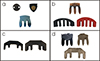 |
Figure 1. (a) performance mutes: Tourte, Alpino, and classical ebony mutes; (b) light practice mutes, weighing less than 35 grams: light metal, black rubber, and red rubber mutes; (c) heavy practice mutes, weighing over 35 grams: heavy metal and rubber-coated heavy metal mutes; (d) altered mute and replicas, weighing over 35 grams: modified classic ebony, lead replica of the classic ebony, and lead replica of the rubber-coated heavy metal mutes. |
2.2 Data acquisition
2.2.1 Sample model
Due to the considerable variations that may occur in the sound production and emission of musical instruments, we adopted a protocol of instrumental execution and recording6 that attempted to standardize as much as possible the records obtained from each reproduction of the sample model, thus allowing comparisons between the different study conditions.
The sample model used in the research consists of a sequence of eight 4 s glissandi per string. The use of glissandi was considered appropriate for this sampling since, in the present study, issues related to variations generated by differences in articulation, dynamics, or phrasing in the intrinsic properties of the instrument's sound are not analyzed. The aim was to extract from the audio, specifically, information about the general harmonic characteristics and the average intensity of the sound radiation of the instruments recorded in a single form of instrumental performance, replicated under different study conditions. Each glissando was performed in a single bow stroke, alternately ascending and descending, driven by a single finger, starting from the open string and ending at its octave, except for the E string, in which the range goes to the B6 (one 12th). So, the samples include 32 glissandi each, from G3 to B6, distributed over the four strings, from low to high. There is an overlap of frequencies (one perfect 4th) between the initial part of each string and the final part of its lower neighbor, except for the G string. This procedure increases the representativeness of the instrument's sound, marked by the specific characteristics of each string. Half of the samples of each study condition were recorded starting with the down-bow and the other half with the up-bow.
The violinists played7 without vibrato, with metronome at 60 bpm (4 beats per glissando), employing détaché8 and using the whole bow9, as loud as possible (preserving the typical sound of the instrument), at a point of contact of the hair bow and the strings halfway between the bridge and the end of the fingerboard, trying to keep the conduction of the bow as regular as possible10.
A DPA condenser microphone, model 4099-DC-1-199-V, with a super-cardioid directional pattern was used for the recordings11. The device was fixed to the instrument using its own clip, positioned approximately 10 cm away from the top of the violin, and pointed at the corner of the bridge. The recordings were made by the participating violinists in 11 sessions, in the same room, always seated in the same position, using the same digital recording equipment, set in the same way.
Each sample generated an audio file, measuring 2:08 min, with a sampling rate of 48 kHz and 24 bits of depth, in mono format.
2.2.2 Audio database
In order to obtain representative data about the effect of mutes, the sampling was reproduced entirely on two violins by four professional violinists, professors, and students from the School of Music at UFMG. For the control condition (without mute), four musicians recorded six takes with each violin, totaling 48 takes. For all other study conditions (use of each of the different mutes), three performers recorded two takes with each violin, resulting in 12 takes. Therefore, since each sample contains eight glissandi on each string, in total, for the control condition, 384 glissandi were recorded per string, and for each study condition, 96 glissandi per string.
2.3 Employed acoustic and psycho-acoustic descriptors
2.3.1 LTAS (Long Term Average Spectrum)
LTAS was considered an appropriate tool for the present study because it provides a representation of the average spectral energy of the analyzed audios, thus allowing the characterization of each study condition. The present study adopted the implementation of LTAS for the MATLAB platform, version 2020a, developed by the Institute of Sound Recording, University of Surrey, England12. A window of 4096 points and a sampling frequency of 48 kHz result in a resolution of 11.72 Hz around the center frequencies of each filter. The spectra were not normalized since the comparative study also involves aspects of sound intensity.
2.3.2 Loudness level
The employment of a psycho-acoustic descriptor, which takes into account the difference in sensitivity of human hearing to sound intensity according to its frequency, allows a better evaluation of the impact of the use of mutes in loudness. Based on the concept of “equal Loudness contours” initially developed by Fletcher and Musson in 1933 [34], the Loudness level makes a specific weighting of the energy registered in the different critical bands encompassed in the audio records. The acousticLoudness function, available in the MATLAB platform, version 2020a13, was used. This function returns a Loudness value in sones for each sample.
2.4 Data processing
The data extracted from the samples were reduced to central tendency values that represent the overall response of the instruments under different study conditions, allowing comparative analyses. All calculations are performed with linear signal amplitude values, and data dispersion measures (e.g., standard deviation) were also calculated to ensure the quality and representativeness of the audio database. After the calculation, the averages are presented in sones (Loudness) and dBFS (LTAS).
However, the Loudness values in sones lack a reference to provide an actual idea of the level of change in intensity caused by the mutes. So, to better evaluate this effect, the percentage of intensity reduction compared to the control condition is presented.
3 Results and discussion
3.1 Sampling control and the results of the two violins
A series of analyses were conducted to verify the efficiency of the instrumental execution protocol in standardizing the executions performed in the different study conditions, such as verification of the melodic lines of the glissandi, comparison between samples starting with the up-bow or down-bow, and also differences observed between the results of the two violins. In general, the samples were considered to have reached a degree of standardization, when comparing the different takes of the same study condition, allowing for a comparative study between the different mutes14.
To analyze the differences between the two violins, a Singular Value Decomposition (SVD)15 of the LTAS matrix was performed with reduced data16 from all control condition samples.
As can be seen in (Fig. 2a), which represents the reconstruction of the main component, with a contribution of more than 90% of the data variation identified in the SVD, there is a significant similarity between the curves of the samples of the two violins, which practically overlap. The other combined components, which in isolation do not present a relevant percentage of contribution to the variations, are reconstructed in (Fig. 2b). Here it is possible to observe different ranges in which the curves relative to the two instruments contrast, indicating a differentiation between the samples of the two violins. This result reflects the typical variation in the acoustic response of each violin, which has specific physical characteristics (woods used, construction details, bridge assembly, etc.) that are responsible for differences in its acoustic response, although the overall curve of every instrument has a common contour close to that of other violins [22, pp. 286 and 287].
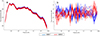 |
Figure 2. (a) Reconstitution of the main component identified by the SVD of the control condition samples and (b) reconstitution of the other components identified in the same analysis. |
To illustrate the impact of these variations on the response of each of the two sampled instruments using mutes, Figure 3 presents the difference in the average LTAS of each violin and of both together in relation to the control condition with the use of two of the devices analyzed, the Tourte mute (a) and the Heavy Metal mute (b). It can be observed that there is a very significant common pattern in both examples between the averages of the two violins for the use of each mute, clearly delimiting the main points of relevance for the study. For example, with both mutes, the two violins present a broad dip in the bridge hill range, more pronounced with the use of the practice mute; in the case of the Tourte mute, there is a slight transfer of energy to the low range of the spectrum (300/400 Hz) in both instruments and, a little more significantly, to the range between 600/1000 Hz; in the case of Heavy metal mute, there is a great loss of energy throughout the low range, outlined by both instruments. On the other hand, in Figure 3a, it can be seen that there are also points of differentiation between the curves; for example, in the range mentioned above of 600/1000 Hz, there are points where the two instruments present peaks or dips at close but distinct frequencies. Likewise, in Figure 3b, there is a variation in the response of the instruments, for example, between 300/500 Hz or between 7000/10 000 Hz, which reflect the particularities of the acoustic response of each violin.
 |
Figure 3. (a) LTAS differences between the control condition and averages of each violin and both violins using the Tourte mute, and (b) LTAS differences between the control condition and averages of each violin and both violins using the heavy metal mute. |
Notwithstanding these particularities of each instrument, as the general contour presented by the average of the two violins presents many more points of convergence than divergence (an effect observed in all the study conditions analyzed), the general results will be presented based on the averages of the two instruments, considering that the present study seeks to trace the average response of the instruments in each study condition and a large number of mutes will be compared.
3.2 Comparison of performance and light practice mutes
The lightest performance mutes17, Tourte and Alpino (Tab. 1), generate little energy transfer to the low region of the spectrum, concentrated in two points: around 380 Hz and 750 Hz; the classic ebony mute, on the other hand, shifts much more energy, however, to lower frequencies, around 270 Hz, a behavior that brings it much closer to the three light practice mutes than to the other two performance mutes (Fig. 4). This behavior can be directly related to the mass of the devices, since this classic ebony mute has a mass similar to the black rubber practice mute (Tab. 1), and the LTAS curves of both are very similar; the other two practice mutes, considerably heavier, shift even more energy to lower frequencies (Fig. 4), which exemplifies the typical effect of mutes described in the literature.
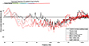 |
Figure 4. LTAS difference between the control condition (without mute) and three performance mutes and three light practice mutes (weighing less than 35 grams). |
Data from the analyzed mutes: performance mutes, light and heavy practice mutes.
Likewise, the reduction in intensity can generally be related to the mass of the devices, even if other physical characteristics also influence this effect (Tab. 1), as can be seen by the percentage of attenuation compared to the control condition (without mute) produced by these mutes: the two lightest performance mutes attain around 23%, the classic ebony mute and the black rubber mute, 28.5% and 27.6%, respectively, and the two other light practice mutes, the red rubber mute and the light metal mute, heavier than the previous ones, 47.4% and 49.2% respectively. The more significant attenuation provided by the two latter mutes can be related to the greater loss of spectral energy observed above 350 Hz with both devices, which do not generate additional small gain peaks between 580 and 800 Hz, differently from all the other mutes depicted in the graph.
3.3 Spectral and loudness changes produced by heavy practice mutes
None of the studied devices weighing more than 35 grams generated a transfer of spectral energy to lower frequencies; on the contrary, all caused a significant energy loss in this region (Fig. 5). The similarity of the five curves is surprising, given the enormous difference in mass between these devices: from the lightest, weighing 37.22 grams, to the heaviest, weighing 168.5 grams, there is a 453% increase in mass (Tab. 1).
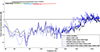 |
Figure 5. LTAS difference between the control condition (without mute) and two heavy practice mutes and three other heavy devices made especially for the study (all weighing over 35 grams). |
There is a clear relationship between the lack of gain in the low frequency region and overall attenuation. All of these heavy devices caused a reduction in the intensity of more than 70%, compared to the control condition. The attenuation provoked by the heaviest practice mute below 35 grams, the light metal mute (Tab. 1), was limited to 49.21%.
It is also noteworthy that there is little variation in the attenuation effect between these devices despite the large difference in mass added to the bridge: the lightest of the five devices produced a loss in intensity of 70%, compared to 81% for the heaviest, which is quite disproportionate considering the substantial variation in mass. Furthermore, it is clear that other factors, such as the type of coupling with the bridge, can influence the degree of attenuation, as exemplified by the lead replica of the classic ebony mute, which attenuated the intensity less than the heavy metal mute and the rubber-coated heavy metal mute, despite being much heavier than the others (Tab. 1).
4 Conclusion
The results suggest that the characteristic effect produced by mutes, which involves transferring spectral energy to low frequencies, only occurs up to a specific mass limit. During the research, other device weighing around 23 grams was analyzed18, which still generated little energy transfer to the low region of the spectrum. The lightest practice mute among the heavy devices presented in this study weighed 37.22 grams (modified classic ebony mute), but the mass limit above which there is no energy transfer is probably lower than that, also conditioned by other physical characteristics of the devices. However, when this mass limit is reached, significant variations in the added mass do not cause a proportional variation in the spectrum, characterizing a functional limit of the bridge, the physical component of the violin effectively altered by mutes.
It can also be concluded that the reduction of energy in the low portion of the spectrum has a decisive effect on the overall attenuation of intensity. While the bridge hill region showed a loss of spectral energy with the use of all the devices analyzed, only the heavy mutes did not cause any transfer of energy to the low portion of the spectrum. These heavy devices were the only ones that achieved more significant overall attenuation rates (above 70%). It was also observed, as with spectral variations, that considerable changes in added mass (over 37 grams) do not cause a proportional change in the attenuation effect.
The article addresses part of a broader research on the effects of mutes on the sound of the violin, which explored a methodology based strictly on the audio analysis of parameterized samples and obtained significant results in differentiating and characterizing the different types of mutes. The choice of this methodology relates to the environment where the work evolved, the School of Music of the Federal University of Minas Gerais, where there was already a great deal of know-how for audio analysis and sampling methodology for musical instruments. Relating the obtained results with the available literature on the acoustic functioning of the violin and the action of mutes, it was possible to establish a theoretical acoustic basis for the observed effects. However, for a complete understanding of the physical acoustic mechanisms by which mutes alter the vibrational behavior of the bridge, for the eventual establishment of a physical model to describe their vibrational characteristics, vibrational measurements (e.g., with an accelerometer) must be performed for each study condition, a crucial step for the continuation of the research.
This study did not analyze the possible effect on playability caused by the use of mutes in general. Although there is no specific mention of this aspect in the reviewed literature, this possibility cannot be ruled out. For example, changes in the bowing force limits required to achieve Helmholtz motion or a modification of attack transient duration can have some effect on playability.
Particularly relevant, in the case of the violin, is the region of the spectrum close to 3000 Hz, strongly influenced by a characteristic resonance of the bridge, known as bridge hill, which directly impacts the acoustic response of the instrument. The bridge hill, resulting from the lateral mobility of the top of the bridge, is so named because it is connected to the interaction between the bridge modes and the violin top plate. Other modes of vibration of the bridge also occur, notably a second mode observed approximately at 6000 Hz, related to the vertical oscillation of the top of the bridge [15, 18–20].
Despite this original concept of use, practice mutes have been used in contemporary music performances due to their particular sound [4].
It seemed not necessary to use any procedure to prevent the samplers from knowing which mute they were using during the recordings since they would not participate in any aspect of the evaluation and analysis of the use of the different mutes, and the use of mutes, regardless of the model, did not produce any difficulty in reproducing the protocol instructions.
Most common and basic bow stroke: the played notes are separated from each other only by the change of bow direction, without interruption other than the change itself.
Average bow travel speed of approximately 16 cm/s.
This performance protocol was designed to fix as much as possible the three main variables that determine the sound response of bowed instruments: the distance from the bridge to the bowing point, the bow speed, and the bowing force (which the musicians often refer to as “bowing pressure”).
Information on the DPA Microphones site available at https://dpa.cloud14.structpim.com/media/4bknjkkj/4099-manual.pdf (Last viewed July 04, 2025).
Code available at https://github.com/IoSR-Surrey/MatlabToolbox (Last viewed January 14, 2025).
Information on the MathWorks site available at https://www.mathworks.com/help/audio/ref/acousticloudness (Last viewed January 14, 2025).
This discussion, with results available in the graphs 4.34 to 4.47, is developed in Section 4.2 in [2].
The SVD function, available in the MATLAB platform, version 2020a, was employed. Information on the MathWorks site available at https://www.mathworks.com/help/matlab/ref/double.svd.html (Last viewed January 14, 2025).
For statistical analysis purposes, the LTAS data of the control condition of the two violins was reduced using the following procedure: starting on the FFT fourth octave (93.8 Hz upwards), the amplitudes of the spectral analysis bins were added together – 2 to 2 in this octave, 4 to 4 in the fifth octave, 8 to 8 in the sixth octave, and so on up to 256 to 256 in the last octave – to obtain a maximum of 4 intensity values per octave. This results in 40 values: 1 for the average of the signal of the section under analysis, 7 for the fundamental frequency of analysis and its multiples up to the third octave (11.7 to 93.8 Hz), and 32 for the remaining octaves. The central frequencies of each band are indicated by the geometric mean between the lowest and highest frequency values contained in each of them.
See [2], pp. 348 and 349.
Acknowledgments
The authors thank the LaPIS team (Laboratory for Performance with Interactive Systems, part of the CPMC – Center for Research in Contemporary Music – and affiliated with the Graduate Program in Music at the School of Music of the Federal University of Minas Gerais, Brazil, in the field of Sonology. Website: https://musica.ufmg.br/lapis/), and especially Professor Ayran Nicodemo.
Funding
This research was supported by the Brazilian research agencies FAPEMIG, CAPES and CNPq.
Conflicts of interest
The authors declare no conflict of interest.
Data availability statement
All audio samples used in this work are available in a Zenodo repository, under the reference DOI: 10.5281/zenodo.15109018.
References
- M.V. da Silva Evangelista: Estudo comparativo do efeito de três diferentes surdinas na sonoridade de seis violinos: alteraçoes na intensidade e no espectro harmônico. Master's thesis, Federal University of Minas Gerais, Belo Horizonte, MG, 2019. http://hdl.handle.net/1843/32235 [Google Scholar]
- M.V. da Silva Evangelista: Análise acústica aplicada ao estudo de surdinas de violino: fundamentos para um protótipo modular multifuncional. Ph.d. dissertation, Federal University of Minas Gerais, Belo Horizonte, MG, 2023. http://hdl.handle.net/1843/65103 [Google Scholar]
- M.V. da Silva Evangelista, S. Freire: Analysis of the influence of different construction factors of violin mutes on their effects: a methodological prospection based on the controlled variation of physical characteristics of the devices, in: 12º Congresso Iberoamericano de Acústica (FIA 2020/22) & 29º Encontro da Sobrac, 2022. https://musica.ufmg.br/sfreire/wp-content/uploads/sites/13/2022/09/marcus-vinicius-freire-fia-2022.pdf [Google Scholar]
- K. Sarch: Con sordino: the art of the mute. American String Teacher 67, 4 (2017) 24–29 [Google Scholar]
- D. Loughridge: Muted violins from Lully to Haydn. Early Music 44, 3 (2016) 427–447 [Google Scholar]
- D.D. Boyden: The History of Violin Playing from its Origins to 1761 and its Relationship to the Violin and Violin Music. Oxford University Press, 1990 [Google Scholar]
- J. Giltay, M. Haas: On the motion of the bridge of the violin, in: KNAW, Proceedings. Vol. 12, 1909, pp. 1909–1910 [Google Scholar]
- P.H. Edwards: A method for the quantitative analysis of musical tone. Physical Review (Series I) 32, 1 (1911) 23 [Google Scholar]
- A. Tyndall, G. White: On the “wolf-note” of the violin and’cello. Nature 98, 2446 (1916) 29 [Google Scholar]
- C. Raman: On the “wolf-note” of the violin and’cello. Nature 97, 2435 (1916) 362–363 [Google Scholar]
- C. Raman: On the alterations of tone produced by a violin – “mute”. Nature 100, 2501 (1917) 84 [Google Scholar]
- C. Raman: Lix. On the wolf-note in bowed stringed instruments. The London, Edinburgh, and Dublin Philosophical Magazine and Journal of Science 35, 210 (1918) 493–496 [Google Scholar]
- C. Raman: Experiments with mechanically-played violins. Proceedings of the Indian Association for the Cultivation of Science 6 (1920) 107–112 [Google Scholar]
- E.V. Jansson, J. Sundberg: Long-time-average-spectra applied to analysis of music. Quarterly progress and status report, 1972 [Google Scholar]
- L. Cremer: The Physics of the Violin. MIT Press, Cambridge, MA, 1984 [Google Scholar]
- C. Gough: Science and the stradivarius. Physics World 13, 4 (2000) 27 [Google Scholar]
- C.E. Gough: Violin acoustics. Acoustics Today 12, 2 (2016) 22–30 [Google Scholar]
- J. Woodhouse: On the “bridge hill” of the violin. Acta Acustica united with Acustica 91, 1 (2005) 155–165 [Google Scholar]
- J. Woodhouse: The acoustics of the violin: a review. Reports on Progress in Physics 77, 11 (2014) 115901 [CrossRef] [PubMed] [Google Scholar]
- G. Bissinger: The violin bridge as filter. The Journal of the Acoustical Society of America 120, 1 (2006) 482–491 [Google Scholar]
- J. Meyer: Acoustics and the Performance of Music: Manual for Acousticians, Audio Engineers, Musicians, Architects and Musical Instrument Makers. Springer Science & Business Media, New York, 2009 [Google Scholar]
- N.H. Fletcher, T.D. Rossing: The Physics of Musical Instruments. Springer Science & Business Media, New York, 2012 [Google Scholar]
- W.M. Hartmann: Principles of Musical Acoustics. Springer, New York, 2013 [Google Scholar]
- E.J. Heller: Why You Hear What You Hear: An Experiential Approach to Sound, Music, and Psychoacoustics. Princeton University Press, Princeton, NJ, 2013 [Google Scholar]
- B. Elie, F. Gautier, B. David: Acoustic signature of violins based on bridge transfer mobility measurements. The Journal of the Acoustical Society of America 136, 3 (2014) 1385–1393 [Google Scholar]
- C.Y. Liang, L. Su, Y.H. Yang, H.M. Lin: Musical Offset Detection of Pitched Instruments: The Case of Violin, in: ISMIR, 2015, pp. 281–287 [Google Scholar]
- D. Loughridge: Timbre Before Timbre. The Oxford Handbook of Timbre, Vol. 269, 2021 [Google Scholar]
- C.E. Seashore: Psychology of Music. McGraw-Hill Book Company, New York and London, 1938 [Google Scholar]
- C.E. Seashore: The psychology of music. XVII. What does the mute do to a violin tone? Music Educators Journal (1938) 23 [Google Scholar]
- K. Kishi: Influence of the weight of mutes on tones of a violin family. The Journal of the Acoustical Society of America 103, 5 (1998) 2916 [Google Scholar]
- C. Ahrens: Metallic mutes used in the eighteenth century. The Galpin Society Journal 60 (2007) 220–119 [Google Scholar]
- T. Tajimi, Y. Soeta, T. Ohsawa, K. Ito: ACF analysis over the open strings’ sound of a violin with and without various mutes, in: UK Institute of Acoustics Day Meeting Sheffield, 2011 [Google Scholar]
- S. Mousavion, S. Sarkar: Empirical study of violin acoustics and its perception under various mutes. The Journal of the Acoustical Society of America 138, 3 (2015) 1935 [Google Scholar]
- H. Fletcher, W.A. Munson: Loudness, its definition, measurement and calculation. Bell System Technical Journal 12, 4 (1933) 377–430 [Google Scholar]
Cite this article as: da Silva Evangelista M.V. & Freire S. 2025. Audio analysis of the effects of heavy violin practice mutes: spectral and loudness changes. Acta Acustica, 9, 45. https://doi.org/10.1051/aacus/2025029.
All Tables
Data from the analyzed mutes: performance mutes, light and heavy practice mutes.
All Figures
|
Figure 1. (a) performance mutes: Tourte, Alpino, and classical ebony mutes; (b) light practice mutes, weighing less than 35 grams: light metal, black rubber, and red rubber mutes; (c) heavy practice mutes, weighing over 35 grams: heavy metal and rubber-coated heavy metal mutes; (d) altered mute and replicas, weighing over 35 grams: modified classic ebony, lead replica of the classic ebony, and lead replica of the rubber-coated heavy metal mutes. |
| In the text | |
|
Figure 2. (a) Reconstitution of the main component identified by the SVD of the control condition samples and (b) reconstitution of the other components identified in the same analysis. |
| In the text | |
|
Figure 3. (a) LTAS differences between the control condition and averages of each violin and both violins using the Tourte mute, and (b) LTAS differences between the control condition and averages of each violin and both violins using the heavy metal mute. |
| In the text | |
|
Figure 4. LTAS difference between the control condition (without mute) and three performance mutes and three light practice mutes (weighing less than 35 grams). |
| In the text | |
|
Figure 5. LTAS difference between the control condition (without mute) and two heavy practice mutes and three other heavy devices made especially for the study (all weighing over 35 grams). |
| In the text | |
Current usage metrics show cumulative count of Article Views (full-text article views including HTML views, PDF and ePub downloads, according to the available data) and Abstracts Views on Vision4Press platform.
Data correspond to usage on the plateform after 2015. The current usage metrics is available 48-96 hours after online publication and is updated daily on week days.
Initial download of the metrics may take a while.