| Issue |
Acta Acust.
Volume 9, 2025
|
|
|---|---|---|
| Article Number | 46 | |
| Number of page(s) | 30 | |
| Section | Inverse Problems in Acoustics | |
| DOI | https://doi.org/10.1051/aacus/2025030 | |
| Published online | 24 July 2025 | |
Scientific Article
Data-driven and physics-constrained acoustic holography based on optimizer unrolling
1
University of Music and Performing Arts Graz 8010 Austria
2
Institute of Electronic Music and Acoustics, University of Music and Performing Arts Graz 8010 Austria
* Corresponding author: This email address is being protected from spambots. You need JavaScript enabled to view it.
Received:
4
December
2024
Accepted:
23
June
2025
Abstract
Nearfield Acoustic Holography (NAH) retrieves vibro-acoustic patterns of sound sources from non-contact measurements of sound in their proximity. NAH obtains images of structural vibrations to analyze the underlying acoustic phenomena. Holographic problems are typically ill-posed and yield infinitely many solutions. Unique solutions are obtained by optimizing a cost function that targets an approximate solution obeying the laws of physics while simultaneously satisfying constraints that represent prior knowledge characterizing the expected result. Which constraints to choose is highly critical for success, and yet the most challenging question to answer. Accuracy fluctuates with the quantity and the quality of these constraints and requires skillful formulation and tuning. Despite ongoing research on novel constraints and parameter tuning methods, as well as rapid advancements in Deep Learning, the state-of-the-art still exhibits substantial deficiencies. As the proposed solution, this article studies a Variational Network for NAH with the idea to fuse physical knowledge with data-driven modeling. The network retrieves the strengths of equivalent sources from measurements by unrolling an iterative optimizer, whose regularizing parameters are inferred via supervised learning. The proposed method outperforms established solvers in a comparative study, using both simulated and real-world data, and it generalizes well to unseen vibration patterns.
Key words: Nearfield Acoustic Holography / Equivalent source method / Data-driven / Physics-constrained / Variational network
© The Author(s), Published by EDP Sciences, 2025
 This is an Open Access article distributed under the terms of the Creative Commons Attribution License (https://creativecommons.org/licenses/by/4.0), which permits unrestricted use, distribution, and reproduction in any medium, provided the original work is properly cited.
1 Introduction
Nearfield Acoustic Holography (NAH) retrieves structural vibration patterns from contactless measurements in the proximity of the vibrating surface using microphone arrays. With the advent and rise of NAH [1, 2] in the 1980s, the inverse sound propagation problem was first described on the basis of the (fast) Fourier transformation on rectangular, flat measurement grids to cope with computational complexity, however implying a periodic spatial repetition and full coverage of the vibration pattern along a flat surface. Another set of methods extended the plane wave expansions of classical NAH to cylindrical or spherical coordinates, e.g. Statistically Optimized NAH (SONAH) [3] and Helmholtz Equation Least Squares (HELS) [4], which are applied on local measurement patches to compensate for the decreased computational efficiency. The Equivalent Source Method (ESM) [5] was later introduced as a versatile, discrete sound propagation model, whose full matrix inversion was enabled by an increase in available computational resources. ESM permits to deal with more arbitrary surface shapes, and the Inverse Boundary Element Method (IBEM) [6–9] could be proposed as a more accurate, quasi-continuous alternative. All of these exemplary achievements apply numerical regularization of the ill-posed sound propagation terms involved [10], e.g. by Tikhonov functional minimization via ℓ2-norm penalty [11], and hereby have to give up on resolving propagating components that are too weak, which causes a blurry image of the surface vibration at low frequencies. And at high frequencies, spatial aliasing causes interference patterns in the image.
In the past decade, methods based on Compressive Sensing (CS) [12–16] have become increasingly popular, as they help to circumvent the inherent spatial blur and moreover allow to relax requirements on spatial sampling. CS requires the surface vibration patterns to be inherently sparse, either directly in space or in a spatial transformation domain [17–29]. Approximate sparsity is commonly enforced by means of ℓ1-norm minimization, which requires non-linear optimization algorithms that trade off between data consistency and sparsity constraint [30]. To guarantee perfect retrieval, the model matrix describing the acquisition process must be sufficiently incoherent [21, 27], which is usually achieved by use of pseudo-random array geometries [18, 19, 21–29, 31]. The use of sparsity has been explored in various domains, as it has been directly applied in the spatial domain [27], in the wavenumber domain (k-space) [21], on modal eigenfunctions [18, 19, 23, 24, 26, 28, 32], and spatial derivatives [25, 33]. While these methods are quite successful and they permit to adapt the solution to the expected source geometries, it is frequently difficult to make a prior choice of the particular criterion that geometrically shapes the solution, as a so-called regularizer. Moreover, spatially extended sources may not always meet a single choice of spatial sparsity condition, and one common sparsifying transformation is often too simplistic. Although CS-based NAH may still be rather successful for sound field retrieval [22], it may also yield non-physical source representations and introduce artifacts, resulting in high reconstruction errors.
In most recent years, Deep Learning [34] has emerged as a new paradigm to solve inverse problems in various domains of imaging, achieving state-of-the-art results in several tasks such as deblurring and deconvolution [35, 36], denoising and impainting [37], super-resolution [38] and CS [39, 40], and it has only recently been introduced in NAH [41–46]. Rather than relying on handcrafted models, these supervised data-driven approaches exploit deep neural networks that, in theory, can learn to approximate any mapping to arbitrary accuracy without the need to formalize prior knowledge and expectations into cost functions. They learn from generic data describing the problem, which avoids leaving optimal parameter and shape decisions up to the user. However, naive application may lack data consistency and the inclusion of acoustic knowledge, so that it rather yields black-box architectures that detach design and training from the known physics of the problem. Ongoing efforts try to improve the explainability of opaque models, such as the Gradient-weighted Class Activation Mapping (Grad-CAM) approach [47]. While this approach yields heatmaps revealing the contributions of the most important input features for the model output, it remains challenging to analyze, interpret, and take responsibility for the network's decisions. Concerning the training effort, exclusion of the scholarly knowledge may yield an overly long training process and requires massive datasets for successful and consistent performance.
For the problem at hand, this justifies putting an increased effort into the question of how to incorporate physical properties of the sound field into learning-based methods, with the idea to enforce fundamental acoustic laws while making neural network decisions more explainable and transparent. Recent literature in sound field estimation [48] differentiates between Physics-Constrained (PCNNs) and Physics-Informed Neural Networks (PINNs) as the two main strategies to embed acoustical knowledge in the architecture and training of the neural network.
On the one hand, PCNNs directly predict as the output the basis function coefficients of discrete and finite wave expansions, e.g. plane waves of the Fourier NAH [49], spherical waves of HELS [50], or equivalent source distributions of the ESM [51], using elementary solutions to the governing Partial Differential Equations (PDEs) of the wave equation. In this way, the learned basis function expansions strictly satisfy the governing PDEs, even if black-box networks are used as the predictors of their coefficients. PCNNs are usually trained on supervised data pairs from which the network learns to infer a model for the given output coefficients to the given input measurement data. The incorporation of elementary solutions is expected to improve estimation accuracy during inference.
On the other hand, PINNs were first introduced to solve forward and inverse PDEs by using the implicit neural representation [52–54] to parametrize the sound field (or other quantities) as a continuous function f(r) in space r=[x,y,z]T to the estimated scalar value g≈f that approximates f at the given coordinates. PINNs learn to represent functions continuously, solely by being trained on discrete samples of these functions. They typically incorporate the physical knowledge encoded by the governing PDEs into the loss function that guides the training process. PINNs based on implicit neural representations are usually trained unsupervised, only using the measurement data without ground truth for training. This makes training feasible when ground truth data is not accessible, which is common for NAH. In that sense, PINNs are trained to fit the measured data while minimizing the deviation from the governing PDEs, such that the estimated sound field approximately satisfies the PDEs. Due to the implicit neural representation, the PDE constraint involved can be evaluated in other locations as the measurement points, which allows implementation of the governing PDEs at high resolution and improves approximation of partial derivatives therein. Ever since their advent, PINNs have been applied in various forms for NAH [55, 56] and sound field estimation in the time [57, 58] and frequency domain [54, 59–62].
This taxonomy of physics-aware approaches greatly helps the discussion but should not be regared as strictly exclusive classification because some methods may meet criteria of both categories. For instance, the Point Neuron Network (PNN) in [54] relies on unsupervised training to learn an implicit neural representation of the sound field, thus can be seen as PINN. As the PNN design does not encode physical knowledge in the loss function but in the architecture, with network weights for strengths and positions of equivalent sources, it can be seen as PCNN. Note that the taxonomy does not make a difference between black-box networks [41–46, 55, 56] and physics-guided architectural designs [54], which incorporate physical models into their neural structure, explicitly.
This paper proposes the use of a PCNN with physics-guided architecture, based on an unrolled optimizer that estimates the NAH image. In particular, a Variational Network (VN) [63–67] is explored as a generative tool for sound source and field retrieval. The proposed VN is built on an unrolled gradient descent scheme with known and learnable parameters that involves generalized data consistency and regularization costs. Unlike typical PCNNs, where only the final network output represents coefficients of the physical basis functions, each VN layer originates from a gradient-descent iteration, returning intermediate coefficients of the equivalent sources as a holographic image. Every VN layer can therefore be regarded a small PCNN. And similar as in [54], the VN architecture directly incorporates the free-space Green's functions as physical fundamental solutions representing the equivalent sources. In contrast to hidden, latent layers, which dominate many neural approaches to NAH [41–46] but are devoid to direct interpretation even if physics are considered [55, 56], the proposed VN is transparent by design: Each layer along the unrolled VN is not latent but delivers a manifest holographic image. The similarity to structurally unrolled iterative solving (see Fig. 1) makes improvement across the manifest layers obvious, providing insights into the VN's decision-making: Improvements of the image are expected to permit interpretation [63–66, 68, 69] in the sense that regularizing constraints as well as domain transformations should be recognized as characteristic improvement patterns across the layers, e.g. relating to sparsity-inducing norms and spatial derivative filters, see also [25, 33]. As the holographic image consists of the strengths of equivalent sources whose radiated sound should not differ much from the input (measurement) data, the VN repeatedly enforces data consistency by penalizing deviations, in every layer. To take into account the complex-valued nature of NAH data, the proposed VN is supposed to perform fully complex-valued operations [56, 70], rather than relying only on magnitude information [41, 42] or treating real and imaginary part separately by stacking them into a real-valued supervector [55]. Ideally, the trained VN should be able to compensate for missing or corrupted information, to find the optimal regularization, and to operate beyond the spatial aliasing limit. For supervised learning, the idea is to present it with a few data sets representative for a large number of vibration images and acquisition setups, in the hope for the network to generalize well to different vibration patterns, changes in measurement distances, and noise levels. Adapting the physical constraints should help minimize the need for problem-dependent regularization or re-training. Geometrically, it is helpful to permit 2D convolutional filter kernels and transformations, and hereby to assume a flat plane for the image/equivalent sources, sampled in a Cartesian (x,y) grid of uniform Δx and Δy increments, parallel to the measurement plane.
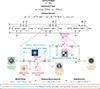 |
Figure 1. Schematic iteration/layer representation of an unrolled gradient descent on a single model mismatch and regularization cost that forms the basis of the Variational Network (VN), showing its structural similarity to a typical residual neural network (ResNet). |
The paper is structured as follows: In Section 2, the ESM and its relation to the forward and inverse problem are explained, along with its inherent ill-posedness and the optimization theory necessary for mitigating its effects to obtain valid solutions. Section 3 recalls the theory behind ill-posed inversion by constrained model fitting and presents some established solvers of NAH in Section 3.2 that are used as benchmarks in this study. Building on this foundation, the VN architecture is derived in Section 4.1, and the PNN in [54] is briefly reviewed in Section 4.2, as it is closely related to the proposed method and thus serves as one more suitable benchmark. Relevant implementation details are presented in Section 5. In Section 6, a simulation study is conducted to investigate accuracy, generalization, robustness, and wideband capabilities of the proposed method by comparing it against the established handcrafted and neural solvers. The study uses spatially extended and compact test sources, including the vibrating plate in Section 6.1, the baffled piston in Section 6.2, as well as the quadrupole in Section 6.3, each representing the contrasting phenomena of smooth variations, constant in-phase vibration and sparsity. Moreover, the iterative nature of the VN allows to observe the holographic image as it evolves across layers/iterations from crude initial approximation to its final outcome, which is investigated in Section 6.4 in a greater detail for the baffled piston example. Section 7 entails an experimental validation of the method to explore its performance under real-world conditions. The experimental source reconstruction concerns a custom-made box with a dispersed loudspeaker layout.
2 Equivalent Source Method (ESM)
We use the Equivalent Source Method (ESM) [5, 71] to model the sound pressure field  of a source sampled in its immediate nearfield across space r=[x,y,z]T in the frequency domain using a planar microphone array of M=Mx·My microphones distributed over the measurement surface SM. According to the ESM, the sound pressure p(rm)=pm at the m-th microphone position rm=[xm,ym,zm]T can be modeled by superimposing the radiated sound fields of a distribution of N=Nx·Ny elementary sources with the weights
  over the equivalent source surface S0, which may be retracted inwards from the structural surface S to prevent singularity. At the angular frequency ω, a single-layer potential driving monopoles (free-field Green's functions) models the sound pressure on the measurement plane, in the discrete-space domain,
 (1)
(1)
Here ρ is the medium density of air, q(r0,n)=qn is the complex source strength of the n-th equivalent source at r0,n=[x0,n,y0,n,z0,n]T, and
 (2)
(2)
is the free-space Green's function that relates the radiated sound pressure at rm to the equivalent source at r0,n, where r=||rm−r0,n||2 is the Euclidean distance between field and source point. Using matrix notation, the problem results in a simple linear equation system
 (3)
(3)
where ![Mathematical equation: $ {{\mathbf {p}}}=[p_1,p_2,\ldots , p_M]^T \in {\mathbb {C}}^M $](/articles/aacus/full_html/2025/01/aacus240143/aacus240143-eq6.gif) contains the discrete sound pressure samples pm of the M microphones,
contains the discrete sound pressure samples pm of the M microphones, ![Mathematical equation: $ {{\mathbf {q}}}=[q_1,q_2,\ldots , q_N]^T \in {\mathbb {C}}^N $](/articles/aacus/full_html/2025/01/aacus240143/aacus240143-eq7.gif) holds as the holographic image the unknown source strengths qn of the N equivalent sources, and
holds as the holographic image the unknown source strengths qn of the N equivalent sources, and  is the propagation matrix, whose entries are the free-field Green's functions in equation (2). The factor jωρ makes q express volume velocities as a measure of source strength, and it is incorporated in G, for brevity.
The holographic goal is to retrieve the equivalent source strengths q from the pressure measurements p by inverting equation (3). This inverse problem yields a source estimate  that can subsequently be used to reconstruct the sound field at any desired point in space outside the source volume by the forward problem equation (3). Correspondingly, the sound pressure pR, (normal) particle velocity vn,R, and intensity In,R reconstructed on the surface SR with zR>z0 become
 (4)
(4)
 (5)
(5)
 (6)
(6)
where GR defines the reconstruction matrix comprised of Green's functions evaluated along the reconstruction points rR,  is the normal derivative with regard to S applied on Green's functions, ⊙ indicates element-wise multiplication (Hadamard/Schur product) and the raised asterisk * denotes the complex conjugate. Note that there is no restriction on the number of reconstruction points rR, so that their number can be chosen in order to define the desired spatial resolution.
3 Ill-posed inversion by constrained model fitting
In practice, the M array microphones that measure p are typically outnumbered by the N equivalent source strengths in q that shall be found. This gives rise to an underdetermined system in equation (3) (M<N) with infinitely many solutions that cannot be solved uniquely. Aliasing problems further increase the ambiguity of the solution. Moreover, the captured signals may be contaminated by noise and other imperfection. In addition, high-frequency vibrational information about the source, carried by evanescent waves that rapidly decay with distance, is lost exponentially the farther the measurement array is placed from the source. This spatial smoothing is modeled by the free-field Green's functions in equation (2), and it would cause an excessive noise boost if the propagator G were to be inverted rigorously, which raises a robustness problem, in practice. All these factors contribute to the ill-posedness of the inverse problem in the Hadamard sense [10], making some form of regularization indispensable and a pre-requisite for accurate reconstruction.
The retrieval of q can be cast into a constrained optimization task that allows to iteratively minimize the mismatch between sound field model and measurements. Additional constraints can be imposed to stabilize the problem. Hereby, the infinite set of possible solutions is restricted to one unique and meaningful estimate that best fits the constraints that aim to model the characteristics of the actual source, while being sufficiently robust to not overfit noisy measurements. One way this can be achieved is by early stopping [72] the iterative model fitting according to some predefined criterion, e.g. after a specified number of iterations. Another, more flexible approach extends the model mismatch to be minimized by an additional penalty term, the so-called regularizer, that constrains the solution in some domain to enforce expected structures or characteristics in the final reconstruction. This results in the variational minimization problem
 (7)
(7)
where  is a data fidelity term quantifying the model mismatch by a scalar mismatch function
  , ℛ(Kq) is the regularizer, usually comprised of some linear transformation
  and scalar penalty function
  , constraining the reconstruction by encoding prior knowledge or assumptions about the source, and λ is the trade-off parameter that controls the balance between minimizing the model mismatch and the constraint. Depending on the choice of K, regularization is either imposed directly on the solution estimate (K=I) or on some linear transformation thereof (K≠I).
Provided that the regularizer is a smooth, differentiable, and convex function, its gradient is defined everywhere, and the objective in equation (7) can be minimized iteratively by gradient descent
 (8)
(8)
for an iteration index t≥0, given some initial q0, where the prime symbol ′ is used to signify the gradient based on the partial derivatives of the estimate q, so that ![Mathematical equation: $ f'(\cdot ) = \nabla _{{{\mathbf {q}}}} f(\cdot )=[\partial f(\cdot )/\partial q_1, \partial f(\cdot )/\partial q_2,.\ldots , \partial f(\cdot )/\partial q_N]: {\mathbb {C}}^N \mapsto {\mathbb {C}}^N $](/articles/aacus/full_html/2025/01/aacus240143/aacus240143-eq20.gif) , the superscript H denotes the Hermitian transpose, and the multiplier τ>0 is the step size by which the coefficients improve towards the negative gradient. A different step size may be allowed in successive iteration steps.
, the superscript H denotes the Hermitian transpose, and the multiplier τ>0 is the step size by which the coefficients improve towards the negative gradient. A different step size may be allowed in successive iteration steps.
3.1 Pre-conditioning
The ill-posedness of the inverse problem to equation (3) typically translates to a large condition number of the propagation matrix G, defined as the ratio between its maximum and minimum singular value, which makes the solution q highly sensitive to small deviations in the measured data p, e.g. due to noise or geometry mismatch. Although regularized iterative solvers as in equation (8) can bypass some of the adverse effects caused by the ill-conditioned matrix G, convergence may still be negatively affected or even infeasible. It is thus common to pre-condition [73] the linear system in equation (3) by transforming it into an equivalent system with more suitable properties for its iterative solution that is easier and cheaper to solve than the original system.
In general, this can be achieved in three ways, which all attempt to reduce the condition number and cluster the spectrum of G. With left pre-conditioning, the problem is modified as
 (9)
(9)
where A is an invertible matrix called left pre-conditioner that operates on the sound field, and that is chosen such that the spectral properties of the factorized matrix A G yield more rapid convergence of the iterative solver. Note that A−1 is intended to loosely approximate G such that, ideally, the pre-conditioned system in equation (9) and the original system in equation (3) approximate the same solution. Similarly, the problem can also be pre-conditioned from the right using
 (10)
(10)
The iterative solver is then used to find an intermediate solution  , from which the final solution
  can be derived in the source domain by applying the right pre-conditioner B. In addition, one can combine both approaches to pre-condition the problem from two sides via split or central pre-conditioning
 (11)
(11)
where the central pre-conditioner becomes M=A B. Which pre-conditioner to use mainly depends on the inverse problem setup and the chosen iterative solver. Provided that suitable pre-conditioners can be found, these modifications can mitigate ill-posedness and accelerate convergence of the used minimization algorithm.
3.2 Traditional solvers
The recent literature provides a variety of established solvers to equation (7) that are all based on different regularization strategies to address the ill-posedness of the problem. These solvers typically aim to minimize equation (7) for a least-squares model mismatch  under individual constraints ℛ(Kq) that geometrically shape the solution according to available prior knowledge. The neural solver to be proposed in Section 4.1 is benchmarked against a reasonable selection of established solvers that have proven effective for sound source retrieval. The benchmarks include the classical Least Norm (LN) [11] and Compressive Sensing (CS) [12–16] solutions, as well as the ones obtained from Total Variation (TV) [25, 33, 74] and its generalization (TGV) [25, 33, 75].
Least Norm (LN)
For the LN solution, the problem in equation (7) is solved by means of a Tikhonov-regularized [11] right inverse
 (12)
(12)
which corresponds to seeking a smooth estimate with minimum energy by use of the λ-weighted  -norm regularizer
  .
.
The LN solution is closely related to the Truncated Singular Value Decomposition (TSVD), which can be robustly computed without matrix inversion as
 (13)
(13)
where  and
and  are unitary matrices whose columns are the left and right singular vectors
  and
and  , respectively, and the diagonal matrix
  contains the singular values
  of the propagator G.
The regularization parameter λ is chosen in a way that the evanescent or weakly propagating components of G associated with vanishing singular values  are either smoothed for LN, or discarded for TSVD, in order to prevent noise amplification due to their inversion.
In their essence, both LN and TSVD are spectral filtering methods based on soft or hard filtering of weak high-frequency components, respectively, which are especially suited for the retrieval of smooth vibration patterns.
Compressive Sensing (CS)
CS [12–16], on the other hand, seeks the sparse solution  with minimal ℓ1-norm, comprised of only few non-zero coefficients. The corresponding minimization problem involving the regularizer ℛ(Kq)=||q||1 lacks a closed-form solution and must be solved by non-linear convex optimization algorithms.
Total (Generalized) Variation (TV/TGV)
Both the LN and CS solutions are considered synthesis priors as they imply desired spatial structures that are directly imposed in the spatial domain (K=I). Alternatively, structural constraints can also be imposed on some transformed domain by analysis priors. A promising choice is to penalize spatial derivatives as they characterize evolution and curvature of the solution in the spatial domain.
In particular, the enforcement of sparse first-order derivatives of the gradient (K=∇=∂x+∂y) by TV [25, 33, 74], which promotes piecewise-constant solutions, has proven effective in modeling uniform in-phase vibrations. Similarly, enforcing sparse second-order derivatives of the Laplacian (K=Δ=∂xx+∂yy) by TGV [25, 33, 75] yields piecewise-linear solutions with minimum curvature, which is well suited for modeling continuous variations as an appealing alternative to LN.
By sparsifying spatial derivatives, TV and TGV tend to produce spatially extended source patterns, which makes them unsuited for the reconstruction of spatially compact sound sources. However, the fusion of TV and TGV with an additional μ-weighted CS constraint for spatial sparsity extends their applicability to compact sources by promoting block-sparse solutions, where non-zero coefficients are not necessarily sparse, but spatially grouped together [25, 33]. In this study, these fused constraints are termed CS-TV and CS-TGV, respectively. The associated regularizers are ℛ(Kq)=||[∇,μI]Tq||1 for CS-TV, and ℛ(Kq)=||[Δ,μI]Tq||1 for CS-TGV, where the weight μ controls the level of spatial sparsity.
4 Neural solvers
Recently, quite some effort has been put into the development of physics-guided neural architectures based on unrolled iterative optimizers. The idea is to design a neural network by unrolling a limited number of iterations of some optimization algorithm that iteratively approximates the solution to a variational problem using prior knowledge. Hereby, each iteration represents one network layer comprised of fixed or learnable update steps that ensure data consistency or act as regularization. Following this concept, Section 4.1 proposes to solve the NAH task with a physics-constrained Variational Network (VN), a term first introduced by Kobler et al. [63] to linguistically capture the close theoretical connection between variational methods and neural networks that guides its architectural design. In particular, the VN architecture is derived from the generalized gradient descent method in equation (8) that solves the variational problem in equation (7) to retrieve the optimal strengths of an equivalent source distribution from ill-posed measurements.
The Point Neuron Network (PNN) [54] is another neural approach to NAH with a physics-guided architecture based on equivalent sources that is closely related to the proposed VN and thus lends itself as a useful additional benchmark; its concept is briefly reviewed in Section 4.2.
4.1 Proposed physics-constrained neural solver based on optimizer unrolling
A generalization of the regularization term in equation (7) is the Fields of Experts (FoE) model [68]
 (14)
(14)
which comprises a linear combination of Nℛ regularizers based on independent linear transformations Ki and scalar constraints  to penalize unfavorable structures in different solution domains with high output values. Instead of using problem-specific, handcrafted transformations Ki and penalty functions ℛi(·), and thereby relying on expert knowledge or assumptions, the FoE model learns parametrized variants thereof from training data.
Under the assumption of Additive White Gaussian Noise (AWGN), the model mismatch in equation (7) is commonly chosen to be a least-squares objective  , with
  being the
  -norm. For x=y=2, it defines a convex quadratic function with a unique global minimum. Relaxing this assumption enables a generalization of the model mismatch [69, 76–78] to a set of
  scalar mismatch functions
  that may as well be parametrized and learned from data. The introduction of learnable split pre-conditioners Ak and Bk as in equation (11) that operate on the field and source domain, respectively, further increases flexibility and may simplify the problem to provide faster and more stable convergence. This yields the generalized model mismatch
 (15)
(15)
Since each summand in equation (15) quantifies an independently pre-conditioned problem, it becomes impractical to minimize the sum total model mismatch w.r.t. an intermediate substitute  from which the final solution
  can be derived as in equation (11), as this requires the inverse problem to be conditioned by a single right pre-conditioner B. Instead, the independent right pre-conditioners Bk are introduced as supplementary domain transformations that provide additional opportunities to learn implicit features from data as in [77]. The use of adaptive mismatch functions and pre-conditioning is supported by ablation studies [76, 78] showing improved reconstruction accuracy due to extended degrees of freedom in data fidelity. This is also backed by other studies of unrolled optimizers [79] that report a substantial performance increase from apt preconditioning, while allowing for a reduced model size and faster training.
Embedding the FoE regularizer in equation (14) and the generalized model mismatch in equation (15) within the variational framework in equation (7) yields
 (16)
(16)
which, under the premise that all functions are continuously differentiable and convex, can be iteratively minimized by gradient descent in equation (8), performing the update
 (17)
(17)
for the iteration index t≥0, given some initial q0.
Proposed Variational Network (VN)
Additional regularization is accomplished by early stopping [72], i.e. truncating the optimization scheme after a pre-defined number of iterations t=T. The use of information from earlier iterates stored in persistent memory [80, 81] is a common means to improve computational efficiency. In particular, the introduction of momentum [82] as a weighted running average of past gradients can further improve estimation accuracy and accelerate convergence by naturally introducing skip connections that improve gradient flow through the network, which has been verified by ablation studies [76, 78]. Unrolling the finite update sequence and letting all adjustable parameters, i.e. domain transformations, penalty functions, trade-off weights, and step-sizes vary across iterations t for maximum flexibility, yields the modified VN architecture [63, 64, 66, 67]
 (18)
(18)
for 0≤t≤T, as shown in Figure 2a, composed of the data fidelity or model mismatch network
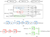 |
Figure 2. (a) The Variational Network (VN) architecture corresponding to equation (18), comprised of (b) the model mismatch network defined by equation (19), (c) the regularizer network defined by equation (20), and (d) the momentum network defined by equation (21). |
 (19)
(19)
in Figure 2b, the regularizer network
 (20)
(20)
in Figure 2c, and the momentum network
 (21)
(21)
with learnable momentum parameters  and
and  in Figure 2d, where the momentum index 0≤l≤t−1 runs from the initial up to the current iteration.
The variant step size τt and regularization weight λt are embedded within the scaling of the gradients for brevity. Passing through the network is equivalent to executing the iterative algorithm a finite number of T times. The algorithm parameters naturally transfer to the network weights θ that are either fixed or learned from training data. This provides the freedom to decide which parameters are best to be extracted from data and which are better modeled according to prior knowledge.
The linear transformations Ki, Ak, and Bk are regarded to be sparse and convolutional, and can thus be realized as complex-valued 2D convolutions over (x,y) with corresponding filter kernels  ,
,  , and
, and  of uniform size d, i.e. Kiq⇔ki*q, Akp⇔ak*p and Bkq⇔bk*q. The propagator G is convolutional by nature and for a planar geometry it is either implemented as a linear layer by direct application of the convolutional matrix G, or as 2D convolution with a fixed Green's function kernel g, i.e. Gq⇔g*q. Under consideration of appropriate boundary conditions and padding [65, 66], the Hermitian transposed operators GH,
  ,
,  , and
, and  can be implemented as complex-valued 2D convolutions with 180°-rotated conjugate filter kernels
  ,
,  ,
,  and
and  , respectively, i.e.
  ,
,  ,
,  , and
, and  . In literature, this operation is often misleadingly referred to as deconvolution, where the overline
  indicates kernel rotation. The respective first-order derivatives of the penalty and mismatch functions
  and
and  act as the activation functions of the network and are applied element-wise on each component of their input arguments.
The unrolled optimization scheme can be considered a T-layer neural network, where each iteration represents one composite layer comprised of residual Convolutional Neural Networks (CNNs) with skip connections; this structural similarity is highlighted in Figure 1 for a simplified VN based on a single model mismatch and regularization cost for sake of clarity. The model mismatch network  and regularizer network
  share a similar structure resembling a symmetric multi-layer CNN with regular and transposed convolutional input and output layers, respectively, that are connected through a tuneable activation layer introducing non-linearity.
In the regularizer network  , the convolutional layers
  and
and  share the same set of Nk linear filters
  (as
(as  ) that are learned from data and vary within and across layers. The same holds for the left and right pre-conditioners
  and
and  , and their respective Hermitian conjugates
  and
and  , in the model mismatch network
  . In contrast, the convolutional layers G and GH use a fixed filter kernel g that is shared across all layers, which is the physics-guided aspect of the network architecture that implements the physics of wave propagation. Moreover, a problem-dependent bias term p in the input layer of the model mismatch network ensures consistency of the solution w.r.t. the measurements.
4.2 Point Neuron Network (PNN)
The Point Neuron Network (PNN) proposed in [54] implicitly satisfies the wave equation, as its fundamental solution, the free-space Green's function in equation (2), is directly embedded into the architectural design. In its essence, the PNN is closely related to the ESM, in that it models an arbitrary sound field p by superimposing the sound radiation of N distributed equivalent sources, termed point neurons, whose complex-valued strengths qn and physical locations r0,n=[x0,n,y0,n,z0,n]T are encoded in the neuronal weights wn and biases bn=[x0,n,y0,n,z0,n]T, respectively, and whose optimal values are inferred from a single set of sound field measurements p via unsupervised learning.
The PNN describes the sound pressure at rm as
 (22)
(22)
which strongly reminds of equation (1) and highlights the analogy wn=jωρ q(r0,n). In contrast to the ESM, the PNN uses a normalized Green's function
 (23)
(23)
to relate a point neuron located at bn to its radiated sound pressure at rm, where the normalization factor
 (24)
(24)
enables modeling of both near- and far-field propagation. However, as this study is mainly concerned with NAH, the normalization factor is readily omitted with χ=1, reducing PN(·) in equation (23) to the Green's function G(·) in equation (2), such that the PNN is governed by the same fundamental equations (1)–(3) as the ESM.
5 Experimental setup
5.1 Setup of traditional solvers
The regularization parameter λ in equation (7) is manually chosen for each method according to the simple, yet effective criterion [29]
 (25)
(25)
which has empirically shown to be a reliable ad-hoc choice for good performance of the solvers in Section 3.2, with option for further fine-tuning. The parameter choice method aims at rejecting singular values of G far below its largest singular value smax for reconstruction, based on an estimate of the given Signal-to-Noise Ratio SNR. The hyper-parameters of the traditional solvers are carefully tuned to optimally fit each source type within their expressive limits. Note that, although the VN is only trained once on a set of representative training data and is then expected to generalize over all test cases, the truncation parameter of its initializer in equation (31) is also set by equation (25) to provide a faithful starting point.
Following the convention in the paper of Fernandez-Grande and Daudet [25], the weight that controls the level of sparsity in the fused CS-TV and CS-TGV constraints described in Section 3.2 is set to μ=1, which offers a good trade-off between spatial and differential sparsity.
In this study, the Fast Iterative Shrinkage-Thresholding Algorithm (FISTA) is used to implement CS, and the Condat-Vu algorithm [83, 84], which is a generalization of the Primal-Dual Hybrid Gradient or Chambolle-Pock method [85], is used to implement TV and its variants. The LN solution requires no iterative approximation but is derived in closed form as in equation (12).
For the TV variants, the first- and second-order spatial derivatives in the gradient and Laplacian are discretized via forward finite differences and implemented as convolutions with 3-point and 5-point stencils, respectively, and zero boundary conditions are used, which consistently provided the best results for all test sources.
5.2 Setup and training of proposed VN
The VN in this study is made up of T=10 layers, resulting in a total of 167 190 learnable complex-valued network parameters  . Table 1 shows the number and dimensionality of the learnable parameters for each VN layer t.
Number and dimensionality of the learnable complex-valued parameters  of each VN layer t.
Convolutional filters
There are many ways to implement the convolutional operations within the network layers (here exemplary shown for the regularizer network). One can treat the complex-valued input q as real-valued entity with twice the size by stacking the magnitude and phase, or real and imaginary parts. Both dimensions can then be separately convolved with either shared [76] or distinct real-valued kernels [64], with the latter doubling the number of parameters. This study, however, adopts the more natural approach of complex convolutions of the input q with complex-valued kernels  s.t.
s.t.
 (26)
(26)
which have been shown to provide quantitative improvements over the split-complex variants [56, 86]. This operation can be performed by a real-valued convolutional layer with two two-channeled kernels ![Mathematical equation: $ k_1 = [k_{\mathrm {re}},-k_{\mathrm {im}}]\in {\mathbb {R}}^{d\times d\times 2} $](/articles/aacus/full_html/2025/01/aacus240143/aacus240143-eq111.gif) and
and ![Mathematical equation: $ k_2 = [k_{\mathrm {im}},k_{\mathrm {re}}]\in {\mathbb {R}}^{d\times d\times 2} $](/articles/aacus/full_html/2025/01/aacus240143/aacus240143-eq112.gif) on the split input
on the split input ![Mathematical equation: $ q = [q_{\mathrm {re}}, q_{\mathrm {im}}]\in {\mathbb {R}}^{N_y \times N_x\times 2} $](/articles/aacus/full_html/2025/01/aacus240143/aacus240143-eq113.gif) , resulting in the output
, resulting in the output ![Mathematical equation: $ [(k_{\mathrm {re}}\ast q_{\mathrm {re}} - k_{\mathrm {im}}\ast q_{\mathrm {im}}), (k_{\mathrm {re}}\ast q_{\mathrm {im}} + k_{\mathrm {im}}\ast q_{\mathrm {re}})]\in {\mathbb {R}}^{N_y \times N_x\times 2} $](/articles/aacus/full_html/2025/01/aacus240143/aacus240143-eq114.gif) from which k*q can be easily assembled [87]. Note that, while keeping the total number of parameters unchanged, complex convolution yields twice as many convolutions as their real-valued counterpart, and thus significantly increases training time. Zero boundary conditions are used to match the conditions imposed on the traditional solvers TV and its variants that rely on convolutions to compute the spatial derivatives.
from which k*q can be easily assembled [87]. Note that, while keeping the total number of parameters unchanged, complex convolution yields twice as many convolutions as their real-valued counterpart, and thus significantly increases training time. Zero boundary conditions are used to match the conditions imposed on the traditional solvers TV and its variants that rely on convolutions to compute the spatial derivatives.
To enhance the expressiveness of the regularizer network and align its structure to the model mismatch network, its convolutional transformation is factorized by two independent transformations K and L, s.t.
 (27)
(27)
The outer convolutional layers, i.e. Li and  in the regularizer network, and Bk and
  in the model mismatch network, use sets of Nℛ=32 and
  filter kernels of uniform size dl=db=5, respectively. While the regular kernels Lk and Bk expand the single-channel input into a Nℛ- and
  -dimensional feature space, respectively, the transposed kernels
  and
and  eventually compress the multi-channel features back into a single source estimate. The inner convolutional layers, i.e. Ki and
  in the regularizer network, and Ak and
  in the model mismatch network, operate on the feature space by applying different sets of Nℛ=32 and
  filter kernels of uniform size dk=da=3 to each extracted feature, respectively, thereby sharing knowledge across channels. Additionally, a least-squares gradient step τtGH(Gqt−p) with trainable scalar step-size τt is used in every VN layer, where left and right pre-conditioners reduce to the identity B=A=I and the activation turns linear
  , which was found to stabilize training. The output layers
  and
and  are depth-wise separable such that their individual feature maps representing gradients can be separately accessed by the momentum network, where they are re-weighted by the scalars
  and
and  before finally being summed up.
Activation functions
Here, potential functions  and ℛ(·) and activations
  and ℛ′(·) are respectively represented by ρ(·) and ϕ(·):ρ′(·) for brevity. Learning the activations ϕ(·) demands differentiable parametrizations that account for the conditions imposed on their associated potential functions ρ(·). Optimization-based NAH typically relies on convex ℓp-norm-based (i.e. p≥1) scalar potential functions
  that define the cost to be minimized with each iteration, and their associated derivatives
  are monotonically increasing vector functions that apply element-wise on their complex-valued argument. However, the aim of the VN is not the successive minimization of a cost, but rather learning a generalized transformation of inputs to desired targets, which allows for relaxation of the convexity constraint, and permits the use of more expressive mappings.
A split-complex approach is often adopted to process the complex-valued input, where activations of real-valued argument  with individual learnable parameters are separately applied to magnitude and phase, or real and imaginary parts. This study, however, considers the use of activations of complex-valued argument and output
  [56, 88, 89].
The activations are applied element-wise ![Mathematical equation: $ \phi _i^t({{\mathbf {q}}})=[\phi _i^t(q_1), \phi _i^t(q_2), \ldots , \phi _i^t(q_N)]^T $](/articles/aacus/full_html/2025/01/aacus240143/aacus240143-eq136.gif) and are realized as parametric interpolators
and are realized as parametric interpolators
 (28)
(28)
using affine combinations of Nw Radial Basis Functions (RBFs) φj(·) with learnable complex-valued weights  and a single bias
  [63–66] per layer t and instance i, which can be written in matrix notation as
![Mathematical equation: $$ \begin{aligned}\phi _{i}^t({{\mathbf {q}}}) &= { {\left [\begin {array}{ccc} \varphi _1(q_1) & \cdots & \varphi _{{\cal {{N}}}_w}(q_1) \\ \vdots & \ddots & \vdots \\ \varphi _1(q_N) & \cdots & \varphi _{{\cal {{N}}}_w}(q_N) \\ \end {array}\right ]} {\left [\begin {array}{c} w_{i1}^t \\ \vdots \\ w_{i{{\cal {{N}}}_w}}^t \\ \end {array}\right ]} } + b_i^t\\ & = \boldsymbol {{\mathrm {\Phi }}}({{\mathbf {q}}}){{\mathbf {w}}}_i^t + b_i^t. \end{aligned} $$](/articles/aacus/full_html/2025/01/aacus240143/aacus240143-eq140.gif) (29)
(29)
Gaussian kernels [90]
 (30)
(30)
are a popular choice for approximating arbitrary functions due to their radial symmetry, smoothness and universal properties [91], and they naturally extend to complex-valued inputs [88]. Here  is the center of the j-th Gaussian that lies on the complex plane, and
  is the real-valued standard deviation that controls its circularly symmetric spread. Note that, although the proposed activations naturally process complex-valued data, the exponential function within the Gaussian kernels in equation (30) still maps to real values
  , which results in real-valued gradients that can negatively affect phase approximation [89]. Alternative Gaussian-like kernels from the class of elementary transcendental functions that provide fully complex mappings
  with complex-valued gradients, such as the hyperbolic secant [89], were also initially considered for more accurate phase retrieval, but were eventually discarded, as their isolated singularities make training prone to instability and divergence.
To optimally cover the input range, RBF centers μj should be equally distributed over an area spanned by the extrema of the complex-valued filter responses (i.e. minimum and maximum real and imaginary parts of  for the regularizer network and
  for the model mismatch network). This is somewhat problematic as they vary across instances i or k, layers t, and training batches, due to constantly changing filter and input statistics – the internal covariate shift [92] – which calls for standardization. Instance normalization [93] has proven effective to stabilize real-valued inputs by forcing channels, which represent the individual inputs of each RBF activation, to follow a standard normal distribution
  with zero mean μ and unit variance σ2 trough channel-wise translation and scaling. In case of complex-valued inputs, one could use a naive implementation, applying instance normalization separately on real and imaginary parts. However, this transformation is not sufficient for the input to follow a standard complex normal distribution
  , with zero mean μ and relation C and unit covariance Γ, as it does not ensure equal variance in both real and imaginary parts and potentially causes the distribution to lose its circular symmetry or become eccentric [94, 95]. A 2D whitening operation was proposed [94] to avoid this problem by directly rescaling the covariance and hereby ensuring circular symmetry of the resulting distribution, which eases adequate sampling of the complex plane with fixed RBF patterns. This is why 2D whitening was adopted, here.
The Nw=64 RBF centers μj are arranged in a sunflower seed pattern [96] that evenly samples the circularly-symmetric input distribution. The spread of the RBFs is derived from the k-nearest neighbors heuristic [97], with the standard deviations σj of the Gaussians chosen as the minimal distance of each center μj to its k=3 nearest centers. While all RBF weights  and biases
  are learned, the centers μj and standard deviations σj of the Gaussian kernels remain fixed to ensure sufficient resolution in all regions of the complex plane throughout the training process.
Initialization
The VN is typically “warm-started” from an initial guess q0 that closely approximates the ground truth based on some inverse transformation of the measurements [81]. This study exploits a right inverse initializer regularized by the TSVD in equation (13). However, following the idea of Schwab et al. [98], the TSVD solution  is extended in a data-driven manner by replacing the truncated singular values
  with non-zero components learned by a neural network
  that are subsequently projected onto the singular vectors that correspond to these truncated singular values, as
 (31)
(31)
Numerical studies [98] prove the superiority of this data-driven continued TSVD q0 over the classical TSVD solution  and justify its use as initializer for the VN to provide a best possible physics-guided starting point. Originally, the data-driven substitute is derived from the TSVD approximation by
  , which is likely suboptimal as
  lacks information about the weakly propagating components one aims to compensate for. In this study, the substitute
  based on the raw measurements p is used, as in equation (31), which still holds information about the evanescent field and is therefore considered a more faithful choice. Moreover, the measurements are typically lower-dimensional than the equivalent sources (M<N), what makes the latter approach more efficient by reducing the number of required parameters and computations in
  . In this study,
  represents a simple 3-layer CNN, where each layer uses a set of
  filter kernels u of uniform size du=5 and RBF activations with Nw=64 Gaussians.
The initial filter and activation weights and biases of the VN are randomly sampled from the complex-valued Kaiming uniform distribution.
Training dataset and augmentation strategies
The network is trained on a randomized supervised training set  of
of  matched source-field pairs
  sampled from the joint distribution of reasonable combinations under the given model
  . The network
  is fed with random batches
  , i.e. portions of the training set, of Nℬ measurement samples
  and related sound field models
  from which it infers source estimates
  that are finally compared to the associated ground truth sources
  by some loss function ℒ(·) providing a reconstruction error to be minimized.
The training data is generated on the fly. It comprises extended and compact source patterns that are fully randomized. Extended vibrational patterns are exclusively created by infinite plates with random material properties that are either resonating or excited by various loads (e.g. point, circle, ring, square) and forces (e.g. uniform, alternating) acting at different locations and frequencies. The linear combination of these simple sources at different amplitudes and phases results in more complex patterns of wave interference. Parametric 2D window functions (e.g. Kaiser, Tukey) with randomized shape parameters simulate different boundary conditions to mimic finite plates. Additionally, compact sources are represented by randomly distributed monopoles. Note that piecewise-constant source strength distributions, such as pistons, are not considered as part of the training data, which keeps the training set small. In Section 6.2, this restriction turns out to be uncritical due to good generalization.
The associated sound field to each source is obtained by application of the forward model G. Networks trained on a specific model setup do not generalize well over different forward models. This is particularly true for changes in measurement distance r, which affect both the exponent and the denominator of the Green's functions in equation (2) contained in the matrix G of equation (3). Training the network on varying forward models Gi, including variation in distance ri and frequency fi, helps to provide generalized information about the physics of wave propagation, which in turn improves regularization. The training data covers the whole frequency range of interest between 20 Hz≤fi≤5 kHz, which exceeds the spatial sampling limit of the equi-spaced array geometry, on purpose. The radiated sound field is evaluated at random distances 1≤zi≤10 cm within the nearfield, to consider different amounts of evanescent waves in the measurements. Furthermore, complex-valued AWGN  with varying SNRi between 25≤SNRi≤50 dB is added to the measurements during training to enforce implicit denoising for more robust retrieval. A varying number of microphones 6≤(Mx,My)≤12 and equivalent sources 21≤(Nx,Ny)≤41 in equation (3) further accounts for different levels of ill-conditioning during training. The introduced randomness acts as data augmentation by exposing the network to a larger variety of source-field pairs without actually increasing the training set of sound sources, hereby preventing the network from overfitting.
Note that, although the network is trained on different sampling densities and measurement distances, equivalent sources and microphones must be kept aligned on parallel planes following regular sampling patterns. Although equivalent sources can theoretically adapt to irregular microphone array geometries and sound sources of arbitrary shapes and orientations (see PNN in Sect. 4.2), it is impractical to learn their optimal setup from supervised data. While some guidelines exist, there is no universal rule for optimizing the number and position of equivalent sources, which makes it difficult to decide on their specific setup for the target reference in training. For this reason, training data does not cover volumetric structures and is rather limited to planar radiators that are discretized on uniform grids of sufficient resolution. Moreover, the inherent structure of the network and training practically limits its use to planar measurement and source structures, as the network heavily relies on 2D convolutions that expect their inputs to have a regular uniform sampling pattern on a planar surface, where each sampling point has a fixed spatial relationship to its neighbors.
Loss and optimizer
Training of deeper networks benefits from layer-wise pre-training, which fits each individual layer output  for 0≤t≤T to the ground truths
  prior to joint training of all layers. The first few layers are then expected to already be close to the optimum, providing good initialization for subsequent fine-tuning [66]. A more integrated approach to pre-training linearly combines layer-wise loss functions and gradually reduces their contribution to the total loss over time according to some regularizing schedule, eventually only leaving the overall loss of the final output layer t=T. Minimizing the exponentially-weighted loss function [76, 77]
 (32)
(32)
has proven effective, where the schedule weight κ0·i≥0, controlling layer penalization, is set to increase with iterations. The initial schedule weight is set to κ0=1e−3. This layer-wise loss function yields faster and stabler convergence by reducing gradient variance across layers, and it significantly reduces the risk of getting trapped in bad local optima. However, it does not increase model complexity and thus not improves reconstruction accuracy, as shown by ablation studies [76].
For the loss ℒ(·) in equation (32) essentially a combined ℓ1-norm is used to summarize the mismatch between magnitude as well as real part and imaginary part between the true and estimated source distribution, as described below.
Additionally, one aspect needs to be considered: In the pursuit of minimizing this loss for sparse sources, the VN tends to drive all equivalent sources to zero early in training instead of concentrating the source strength at the origin of the sound. As CNNs are known to be biased towards smooth solutions before learning fine-grained details and sparse patterns, they yield huge reconstruction errors for point sources at the early stages of training. Simply zeroing the output seems to be an easier task and minimizes the loss faster than concentrating the energy spread in only a few active coefficients, and once the output is zeroed, point sources cannot be recovered later in training. As a remedy, the Normalized Cross Correlation (NCC)
![Mathematical equation: $$ \epsilon _{\mathrm {NCC}} = \frac {|{{\mathbf {q}}}^H \cdot {\hat {{{\mathbf {q}}}}}|}{||{{\mathbf {q}}}||_2 \cdot ||{\hat {{{\mathbf {q}}}}}||_2} \in [0,1] $$](/articles/aacus/full_html/2025/01/aacus240143/aacus240143-eq177.gif) (33)
(33)
is used as an auxiliary loss to capture the similarity between estimate and ground truth while compensating for local variations induced by scaling and bias. This hinders the suppression of all source activity by preserving structural similarity. Since ϵNCC=1 indicates a perfect match, the resulting loss becomes
 (34)
(34)
and is used for the layer-wise loss in equation (32), which is iteratively minimized until convergence for 100 k iterations in batches of Nℬ=8 samples using the Nesterov-accelerated Adaptive Moment Estimation (NAdam) optimizer. A scheduler reduces the initial learning rate ζ=1e−3 whenever training plateaus, and gradient clipping is used to stabilize convergence. Once the network is trained, the learned parameters  are fixed, and new, unseen measurements of similar nature can be fed to the network
  that then serves as optimal reconstruction operator for data-driven source retrieval.
5.3 Setup of PNN
Instead of relying on supervised training on labeled datasets as the VN, the PNN follows the paradigm of unsupervised “one-shot” learning by directly fitting the model to a single set of array measurements. Such unsupervised methods [99–107] can be more efficient and become appealing when data is scarce, which is common for large-scale microphone array systems, but they are typically more prone to overfitting to measurement noise. Different strategies to mitigate overfitting have been proposed, including early stopping [100], the use of underparametrized network architectures [99, 107], and additional denoising regularizers [103, 104]. The PNN relies on the use of weight regularization, using a sparsifying model complexity loss [54], combined with early stopping [72]. For simulation experiments, where the ground truth of the source is available, training is stopped as soon as the ϵRMSE between the estimated and true source distribution starts to monotonically increase, which indicates overfitting.
During training, the model parameters ![Mathematical equation: $ [{{\mathbf {w}}}, {{\mathbf {B}}}]=[w_0,\ldots ,w_N, {{\mathbf {b}}}_0,\ldots ,{{\mathbf {b}}}_N]\in {\mathbb {C}}^{4N} $](/articles/aacus/full_html/2025/01/aacus240143/aacus240143-eq181.gif) , and thereby the strengths wn=qn and locations bn=r0,n=[x0,n,y0,n,z0,n]T of the equivalent sources, are iteratively updated by backpropagation, minimizing the regularized loss function
, and thereby the strengths wn=qn and locations bn=r0,n=[x0,n,y0,n,z0,n]T of the equivalent sources, are iteratively updated by backpropagation, minimizing the regularized loss function
![Mathematical equation: $$ \left [{\hat {{{\mathbf {w}}}}}, {\hat {{{\mathbf {B}}}}}\right ] =\arg \min _{[{{\mathbf {w}}}, {{\mathbf {B}}}] \in {\mathbb {C}}^{4N}} \left\{ ||\mathrm {PNN}({{\mathbf {G}}}, {{\mathbf {w}}}, {{\mathbf {B}}}) - {{\mathbf {p}}}||_2^2 + \psi ||{{\mathbf {w}}}||_1 \right\} $$](/articles/aacus/full_html/2025/01/aacus240143/aacus240143-eq182.gif) (35)
(35)
comprised of the least-squares model mismatch  and a spatial sparsity constraint ψ||w||1 as the model complexity loss that controls the number of active equivalent sources to avoid overfitting to the noisy measurements p.
In light of the ESM, the minimization problem in equation (35) fits in the variational framework of equation (7) under CS constraints as described in Section 3.2, with the main difference being the trainable locations of the equivalent sources B, which act as kind of regularization, and the use of backpropagation instead of classical gradient descent to update the model parameters.
Initialization
The authors of [54] suggest the initial weights w0 and biases B0 of the PNN, that respectively represent strengths and distribution of the equivalent sources, to be determined based on prior knowledge about the underlying physical scenario and model parametrization, as this speeds up convergence and avoids getting trapped in local minima. Moreover, equivalent sources must neither be placed on the source surface nor the measurement points, as otherwise gradients for backpropagation become infinity. Following these suggestions, the equivalent sources are equidistantly placed just beneath the source surface, using a small retreat distance of z0,n=−1 mm to prevent singular gradients, and the source strengths encoded in the network weights are initialized with the LN solution  of equation (12). This allows for a fair comparison between the PNN and the VN, which exploits a similar approximate solution of equation (31) as a starting point.
Hyperparameters
For training, the PNN requires a manual choice of gradient step sizes for the weights w, as well as for each of the Cartesian coordinates in the biases bn=[x0,n,y0,n,z0,n]T, except for z0,n, which remains fixed at z0,n=−1 mm ∀n∈N, on purpose. Moreover, one has to choose the weight ψ of the sparsifying model complexity loss, as well as the regularization weight λ of the LN initializer, which is determined according to equation (25). These hyperparameters must be carefully tuned for the problem at hand, and their optimal values are vastly different for the individual test cases that follow. By contrast, the trained VN requires no manual tuning of parameters, and it generalizes well to different scenarios without the need for human intervention.
6 Comparative simulation study
A simulation study is conducted to examine the strengths and weaknesses of the proposed VN by comparing it to the established traditional techniques of Section 3.2, and the more recent neural PNN approach of Section 4.2, for sound source and field retrieval. Note that, to date, the PNN has only been investigated for sound field estimation [54], yet the underlying source distribution encoded in the network weights remains unexplored; a gap this study happens to close. Reconstruction quality for different source types and frequencies is investigated via visual inspection, as well as objective quality metrics. The metrics include the normalized Root Mean Squared Error (RMSE)
![Mathematical equation: $$ \epsilon _{\mathrm {RMSE}} = \sqrt {\frac {\sum _{i} (x_i - {\hat {x}}_i)^2}{\sum _{i}x_i^2}} = \frac {||{{\mathbf {x}}}-{\hat {{{\mathbf {x}}}}}||_2^2}{||{{\mathbf {x}}}||_2^2} \in [0,1], $$](/articles/aacus/full_html/2025/01/aacus240143/aacus240143-eq185.gif) (36)
(36)
where x is the ground truth reference and  is the estimated acoustic quantity representing either source strength q, sound pressure p, (normal) particle velocity vn or intensity In, as well as the NCC as in equation (33), the Structural Similarity Index Measure (SSIM) [108], and the Peak Signal-to-Noise Ratio (PSNR). Note that all metrics are shown as percentages by multiplying them by 100%, except the PSNR, which is expressed in decibels (dB). The quality metrics for each method are presented underneath the source estimate in the associated subfigure. The test sources cover as the most basic source types the vibrating plate in Figure 3a, the baffled piston in Figure 3b, and the quadrupole in Figure 3c. Each of these represent either a spatially extended or compact source pattern. These patterns comprise the contrasting phenomena of smooth variations, constant in-phase vibration, and sparsity, making them best suited for exploration of the network's generalizability. What is more, the effects of measurement noise and aliasing on the solution accuracy become apparent. Finally, the iterative nature of the VN and its benchmarks allows to compare their iterative evolution for the example of the baffled piston by assessing intermediate equivalent source estimates, both visually and in terms of objective quality metrics, as they evolve across layers/iterations from a crude initial approximation up to the final solution.
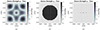 |
Figure 3. Ground truth equivalent source distributions for the (a) center-driven plate in Section 6.1, (b) baffled piston in Section 6.2, and (c) quadrupole in Section 6.3, that are used as references in the simulation study of Section 6. |
Obviously, traditional solvers may fail by design to deliver useful reconstructions in irregular cases, where the structural constraint (e.g. sparsity) does not hold for the given ground truth characteristics (e.g. smoothness). This particularly concerns (i) LN for the sparse quadrupole, and CS for (ii) the plate and (iii) the piston. Excluding these three irregular cases, the imaginary part remains negligible compared to the real part of all estimates, as outlined by a limited Imaginary-to-Real Ratio
 (37)
(37)
that regularly assumes values below IRR<−20 dB, considering only strengths q of equivalent sources whose magnitude |q| exceeds 5% of the maximum strength |q|max. Consequently, we discard an investigation of the phase and rather focus on the magnitude of the retrieved source strengths.
All testing data are generated under the same model setup. The equivalent source model is realized as single-layer potential of Nx×Ny=41×41→N=1681 equidistant monopoles that are uniformly placed on the surface of the radiator at z0,n=0 m, spanning an area of 50×50 cm2. The radiated pressure field is sampled at a measurement distance of zm=6 cm by a Mx×My=8×8 equi-spaced square array of M=64 virtual microphones whose area is parallel to the 50×50 cm2 source plane and fully covers it. The microphone spacing of Δx,Δy=7.143 cm results in a spatial sampling limit around f=c/(2Δx)=2401 Hz, where c=343 m/s is the speed of sound in air at 20 °C, beyond which aliasing can be expected. All simulated measurements are corrupted by complex-valued AWGN with SNR=28 dB drawn from a fixed random seed for a fair comparison.
6.1 Center-driven plate
Let's first consider the reconstruction of a simply supported aluminum plate of thickness h=5 mm that is center-driven at the origin (x,y)=(0,0) m by a point force oscillating at f=800 Hz. The maximum source strength is normalized to Qmax=1 m3/s. The material-specific constants include Young's modulus E=69 GN/m2, Poisson's ratio ν=0.334, and a density of ρ=2712 kg/m3. The radiated pressure field is sampled and traced back to the source surface using the VN and its benchmarks. Figure 3a shows the ground truth and Figure 4 shows the reconstruction estimates of the center-driven plate.
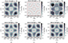 |
Figure 4. Equivalent source reconstructions of the center-driven plate in Figure 3a vibrating at f=800 Hz based on (a) LN, (b) CS, (c) TV, (d) TGV, (e) PNN, and (f) VN, retrieved from measurements with SNR=28 dB taken at a distance of zm=6 cm. |
The LN estimate in Figure 4a captures the characteristic shape of the modal pattern, but suffers from significant warping artifacts and side lobes due to the measurement noise, which become most apparent towards the plate margins when compared to the ground truth in Figure 3a. The minimum energy constraint causes a smearing of source activity, especially across the edge nodal lines, which spoils symmetry. Although peak magnitude is rather accurate, the energy distribution of the individual modes does not fully agree with the ground truth and local magnitude tends to be underestimated, particularly around the center.
The sparse solution obtained by CS in Figure 4b cannot retrieve the continuous variations of the modal pattern, but rather decomposes it into sparse clusters of point sources that are situated around the modal peaks.
TV in Figure 4c provides a piecewise-constant estimate with sparse gradients that only coarsely resembles the true modal pattern. While one can sense the contours of the mode shape, it is inadequately resolved and suffers from the well-known staircase effect, where smooth variations are approximated by step-like functions. The individual modes appear flat and overly rounded, with the corner modes displaying pronounced side lobes induced by the measurement noise. There is misleading source activity across all nodal lines, as neighboring modal peaks and valleys tend to merge to a common plateau, ensuring minimal variation in magnitude with only few non-zero gradients. Due to the constant energy spread, the peak magnitude is slightly underestimated.
TGV in Figure 4d successfully recovers the smooth variations on the plate, producing a well-resolved source that closely approximates the ground truth with piecewise-linear functions. Compared to LN in Figure 4a, it appears more robust to the measurement noise, showing a lower level of warping and side lobes. Despite the use of zero boundary conditions, which greatly improved reconstruction accuracy at the plate's borders, there still remains misleading source activity across the edge nodal lines. The energy distribution of the individual modes is more concentrated around their peaks, showing less energy smearing and a more steep and steady slope due to the minimum curvature constraint. This also causes considerable local overestimations in magnitude. Nonetheless, TGV seems an appropriate choice for the reconstruction of the mode shape.
The PNN in Figure 4e takes the LN estimate of Figure 4a as initial approximation and iteratively refines it during training by adjusting the strengths and positions of the equivalent sources under a spatial sparsity constraint. After training, the equivalent sources are no longer uniformly arranged on the source plane, but oriented in a way that makes up for some modeling errors of the LN. The learned source positions are not explicitly displayed here as they may warp the reconstructed source distribution. Instead, to ease visual comparison, the non-uniform equivalent sources are interpolated onto the same regular grid as used throughout this study using linear barycentric interpolation, which provides sufficient accuracy for the dense spatial sampling. In general, the PNN and LN solutions share the same characteristics, but the rearranged sources yield more pronounced magnitude for the modal peaks, particularly in the center, as well as reduced activity at the edges of the plate. The latter is further encouraged by the spatial sparsity constraint in the model complexity loss, which helps to combat noise but must not be too strict and rather carefully tuned to not overly suppress source activity as in the CS solution in Figure 4b. Altogether, the accuracy of the PNN only marginally exceeds the traditional solvers and strongly depends on the correct choice of hyperparameters during training.
The VN in Figure 4f clearly outperforms its benchmarks, which is reflected by the quality metrics. It seems remarkably robust to the measurement noise as the reconstruction shows almost no deformations or artifacts. The structural characteristics of the modal pattern are nearly perfectly retrieved and nodal lines are mostly free of any source activity. The magnitude distribution closely matches the ground truth, with only the center deviating, which is a common problem among all tested methods. Noise suppression at the borders is significantly improved by simulating different boundary conditions for the reference plates during training, as well as the use of zero boundary conditions for convolutions. Against expectations, this does not negatively affect the retrieval of (infinite) plates, where structure-borne waves expand well across the aperture of the measurement array.
6.2 Baffled piston
Let us now consider the vibrating circular piston in Figure 3b of the diameter ∅=40 cm mounted in the center (x,y)=(0,0) cm of a rigid baffle. Again, the source strengths are normalized to a maximum of Qmax=1 m3/s. The estimated sources are then used to reconstruct the sound field in terms of sound pressure pR, normal velocity vn,R, and intensity In,R according to equations (4)–(6) at a distance of zR=3 cm above the source plane. The retrieval is conducted over a frequency range from 100 Hz−5 kHz in 100 Hz increments, purposely exceeding the spatial sampling limit to test the methods for wideband reconstruction. Figure 5 illustrates the estimated source distributions for an exemplary frequency of f=1 kHz.
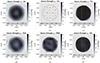 |
Figure 5. Equivalent source reconstructions of the baffled circular piston in Figure 3b vibrating at f=1 kHz based on (a) LN, (b) CS, (c) TV, (d) TGV, (e) PNN, and (f) VN, retrieved from measurements with SNR=28 dB taken at a distance of zm=6 cm. |
LN in Figure 5a and TGV in Figure 5d accurately retrieve the circular shape of the piston, but they fail to capture the spatial extent and constant magnitude of the piston area, as both methods imply smooth variations. Instead, the estimated sources remind more of a circular plate mode, with the center suffering from a notable drop in energy, creating a ring-like appearance. The piston estimates are also accompanied by spurious side lobes, indicating poor suppression of measurement noise, which reflects in the quality metrics. However, both methods reliably reconstruct the investigated sound field quantities at f=1 kHz within reasonable errors, as shown in Figures 6b–6d.
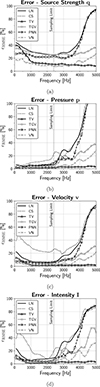 |
Figure 6. Ensemble-averaged ϵRMSE as in equation (36) in percent for the (a) reconstructed equivalent sources of the baffled piston, retrieved from measurements with SNR=28 dB taken at a distance of zm=6 cm, along with their radiated (b) sound pressure, (c) normal velocity, and (d) normal intensity field reconstructed at a distance of zR=3 cm, as in equations (4)–(6). The vertical line at f=2401 Hz marks the spatial sampling limit. |
The sparse solution of CS in Figure 5b does not conform with the physical structure of the piston, but inadequately represents it by a dispersed cluster of monopoles, merely hinting its true spatial extent. Active equivalent sources are distributed in a regular pattern within the limits of the piston, with only few outliers, which is dictated by the uniform spatial sampling protocol. Switching to a pseudo-random sampling scheme is often done for CS to reduce the number of microphones while maintaining accuracy, and it repositions the point sources according to the used array geometry. It is noteworthy that this sparse estimate still yields accurate radiation of the acoustic pressure in Figure 6b within reasonable errors, as it is explicitly matched by the CS algorithm. This is made possible due to the Green's functions in equation (2) in the propagator G, which act as a spatial blur, thereby creating smoothly varying sound fields, even for sparse sources. As the sound field is expressed as a superposition of sound fields due to each equivalent source, the sparse source cluster radiates with exceedingly high strength levels to compensate for the lack of continuous source activity along the area of the piston to generate a pressure field of similar magnitude. Nonetheless, the retrieval of the sound particle velocity in Figure 6c and intensity in Figure 6d still yields intolerable errors, as these quantities are not explicitly matched by the CS algorithm.
TV in Figure 5c promotes sparse spatial gradients and thereby creates a sharp-edged solution with piecewise-constant magnitude, which is an excellent fit to the flat piston source. The spatial extent of the piston is accurately captured, although some edges appear tapered. Despite the good noise suppression, the sparsification of gradients tends to fuse adjacent artifacts induced by the measurement noise into larger patches of constant magnitude, as can be seen in the area surrounding the piston. However, these artifacts are negligible and do not notably degrade reconstruction. In short, source and sound field retrieval by TV is remarkably accurate for all acoustic quantities of interest, making it the state-of-the-art handcrafted approach to infer constant in-phase vibration.
Although the PNN solution in Figure 5e is based on the rather poorly performing LN in Figure 5a, it provides a more adequate (interpolated) estimate of the piston with a sharply defined edge and a more homogeneous magnitude distribution on its area. Peak magnitude is overestimated and comes close to the TGV in Figure 5d. The reordering of equivalent sources causes the center gap suffered by LN (and TGV) to disappear at the cost of introducing a small ripple surrounding the center. Moreover, it loosens the smoothness constraint of LN and tolerates sharper edge transitions while maintaining the spatial extent, with only a few local exceedances. The additional spatial sparsity constraint limits the number of active equivalent sources and thereby enforces an almost noise-free baffle, which significantly improves all quality metrics. Note that, generally, the fusion of any traditional solver with a carefully tuned spatial sparsity constraint, as for example in the CS-TV and CS-TGV methods described in Section 3.2, likely yields the same level of noise suppression. The reconstruction accuracy of the sound field at f=1 kHz is en par with LS and TGV, but clearly falls short against TV, as seen in Figures 6b–6d. Nonetheless, the PNN turns out more advanced than most traditional solvers, and flexible enough to approximate not only smooth curvature, as in Figure 4e, but also the piecewise-constant one in Figure 5e within reasonable errors.
The neural solution produced by VN in Figure 5f even surpasses the accuracy of TV by not only providing a constant magnitude distribution close to unity that is strictly limited to the contour of the piston, but also an entirely artifact-free baffle due to superb noise suppression. This is despite the solution builts upon the initial LN estimate in Figure 5a that is inherently smooth and suffers from various deficiencies, which are fully compensated by the network. This result for VN becomes even more impressive when considering that it is exclusively trained on smooth and sparse source distributions, not actively taking piecewise-constant vibration patterns into account, which highlights VN's potential to generalize to unseen data. Moreover, the VN seems less prone to undesirable spatial blur or staircasing, as it reliably preserves the sharp edges of the piston. The use of randomly parametrized spatial window functions of different aperture during training, with roll-offs ranging from smooth to sharp, presumably conditions the network to precisely discriminate between different source boundary types. Despite its remarkable accuracy for source retrieval, the VN estimate does not reconstruct the sound field as faithfully as TV, but is rather en par with LN and TGV, as shown in Figures 6b–6d. Although the source estimate seems a more appropriate fit in terms of magnitude, its complex-valued components may diverge from the ground truth, which negatively impacts sound field retrieval.
The Figure 6 shows the methods’ reconstruction error for sound source and field retrieval over frequency. For each frequency, an ensemble averaged error over ten randomly seeded noise realizations with SNR=28 dB is provided. Most of the insights gained from investigating the methods at a particular frequency can be extrapolated well to other frequencies.
The first thing to be noticed is that CS retrieves sparse estimates with reconstruction errors so large that they cannot even be displayed in Figure 6a within the illustrated source error range, as the ground truth itself is all but sparse. However, as already noted, these estimates still radiate pressure fields within reasonable errors, at least for frequencies below the spatial sampling limit in Figure 6b, which cannot be claimed for sound particle velocity in Figure 6c and intensity in Figure 6d, whose errors are significantly higher.
Another point standing out is that, despite significant differences in absolute error, all methods share a similar relative error trend.
At frequencies below the spatial sampling limit, one can observe in Figures 6a–6d a gradually increasing error towards lower frequencies below 1 kHz, which is least pronounced for the neural solvers PNN and VN considering all acoustic quantities. This trend can partly be explained by a loosening of the regularization constraint, whose weight, dictated by equation (25), is proportional to the largest singular value smax of the propagation matrix G, which decreases with frequency. This shows that, although the piecewise-constant magnitude constraint of TV generally seems a perfect fit for piston retrieval, the ad-hoc parameter choice turns out insufficient and requires manual tuning to achieve optimal results under changing conditions. In contrast, the self-regulating layers of VN, as well as the readjustment of equivalent source strengths and positions by PNN, both make up for the unsuited regularization of their LN-based initializer, which also depends on equation (25) and thus suffers from over-regularization, with the VN consistently providing the least reconstruction error at low frequencies.
An even greater net increase in error can be observed towards higher frequencies above the spatial sampling limit, where aliasing starts to occur; except for TV, which knowingly suppresses aliasing effects to a significant extent [25]. Soon after exceeding the sampling limit, errors of LN, CS, and PNN in Figures 6a–6d rapidly increase as the methods are not capable of wideband reconstruction. While at low frequencies, equivalent source activity is primarily found within the boundaries of the piston, with only occasional outliers, it starts to spread across the baffle at high frequencies due to a mixture of measurement noise and aliasing. As cardinality increases and more equivalent sources contribute to the sound field, peak energy rapidly decreases as a consequence. Ultimately, the retrieved estimates dissolve into a noisy source distribution, not even resembling a vague shape of the piston, anymore. By contrast, TGV, TV, and VN all combat aliasing effects and suppress noise much more reliably, producing estimates whose source activity stays mainly concentrated at the piston's area, even at very high frequencies. It is remarkable that, although VN is built upon the LN solution that is susceptible to aliasing, the network is able to compensate under-sampling artifacts and to produce a well-preserved piston estimate within reasonable errors, even at frequencies where reconstruction errors of LN diverge. Although PNN also adapts the initial LN distribution, and thereby reduces its error to some extent, it relies on rather simple regularization trough spatial sparsity and repositioning of equivalent sources that appears insufficient to notably limit the rapid error increase towards high frequencies. This highlights the need for more advanced regularization techniques, as used by VN, to deal with aliasing and enable reliable wideband reconstruction beyond the spatial sampling limit. Ultimately, however, aliasing effects dominate at high frequencies and even the solution of VN starts to slowly break down. Far beyond the spatial sampling limit, only TV provides stable reconstruction with minimal error, which even seems to decrease further with increasing frequency.
In the mid frequency range between 1 kHz and slightly above the spatial sampling limit, where regularization is close to optimal and aliasing does not dominate yet, the similar error of 10−20% for TV and VN subceeds the error of all competing methods by at least 10%, as depicted in Figure 6a, which again highlights the importance of a suitable choice of constraints for source retrieval. In this frequency span, TV and VN both provide piecewise-constant estimates which closely resemble the ground truth and thus result in minimal reconstruction errors below 15%, with VN consistently yielding the best results until 3.5 kHz. However, all methods except CS perform similarly well for sound field retrieval in Figures 6b–6d, providing errors below 10% with only minimal difference. Even though VN yields the best approximation of the ground truth in terms of magnitude, real and imaginary components may differ to a larger degree compared to TV, causing slightly worse sound field reconstruction metrics.
6.3 Quadrupole
The accurate localization of compact sources is a common yet difficult task in acoustic holography that many popular methods struggle with. To evaluate the performance on localizing point sources, the longitudinal quadrupole in Figure 3c of length l=16 cm, composed of three monopole sources, with the middle one oscillating at f=3 kHz with twice the amplitude and inverted phase, is placed at the center (x,y)=(0,0) cm of the source plane. The volume velocity of the center monopole is Qc=−1 m3/s, resulting in a source strength of Ql,r=0.5 m3/s for the two adjacent point sources. The predicted equivalent source strengths for the quadrupole source are shown in Figure 7.
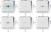 |
Figure 7. Equivalent source reconstructions of the longitudinal quadrupole in Figure 3c vibrating at f=3 kHz based on (a) LN, (b) CS, (c) CS-TV, (d) CS-TGV, (e) PNN, and (f) VN, retrieved from measurements with SNR=28 dB taken at a distance of zm=6 cm. CS-TV and CS-TGV use unity weight μ=1 for the spatial sparsity constraint. |
For an accurate approximation of a point source, the solution must be sufficiently sparse in space. CS in Figure 7b directly enforces spatial sparsity and thus yields the most accurate solution. It reveals the correct locations of the monopoles and closely approximates their true magnitude level, as it concentrates the solution energy in very few non-zero coefficients.
By contrast, LN in Figure 7a tends to evenly spread the solution energy across multiple coefficients throughout space, producing sinc-like spatial responses to point sources which extend over a large area. As a consequence, the solution suffers from high levels of side lobes surrounding three broad main lobes enclosing the true source locations, which impedes correct localization. Moreover, the energy spread yields a severe underestimation in magnitude, resulting in very high reconstruction errors.
The solution obtained by TGV (not shown for brevity) is reminiscent of the LN solution in that it shows spatially extended, smooth magnitude variations around the true source positions. However, the introduction of additional spatial sparsity by CS-TGV in Figure 7d significantly narrows down the width of the main lobes while suppressing all side lobes and noisy artifacts and hereby significantly improves source localization and separation. The resulting energy surplus in the main lobes drives the peak magnitude closer to unity, but there still remains a substantial mismatch. By putting more emphasis on the spatial sparsity constraint, one can narrow the lobe width and boost the magnitude even further, hereby approximating CS at the expense of giving up on the piecewise-linear characteristics that constitute TGV. Optimal regularization is only achieved by careful manual tuning of the hyperparameters.
CS-TV in Figure 7c behaves akin to CS-TGV in terms of peak magnitude, noise suppression and narrowing of the quadrupoles main lobes, but the smooth variations are replaced by sharp-edged patches of constant source strength. The number of active equivalent sources is slightly reduced, which further enhances localization.
Starting from the LN solution in Figure 7a, the PNN in Figure 7e faithfully locates the quadrupole by accumulating most of the source strength in only a handful of active coefficients directly adjacent to the true monopole positions. Although peak magnitude of PNN exceeds CS-TV in Figure 7c and CS-TGV in Figure 7d nearly threefold, which greatly improves scale-related error metrics, it is still substantially lower than the ground truth in Figure 3c. Similar to CS in Figure 7b, the spatial sparsity constraint is vital for suppressing most of the source activity outside the span of the quadrupole, and therefore the weighting of loss functions is heavily biased towards the sparsity-inducing model complexity loss in equation (35). On a closer look, despite the sparsity bias, source strengths of the PNN do not fully vanish in source-free regions, but they are rather conserved in low-level residuals of the side lobes that degrade the initial approximation by LN. Moreover, the less an equivalent source contributes to the modeled sound field that loosely matches the measurements, the less likely it moves from its initial position during training. Consequently, the need for sparsity essentially bypasses repositioning of the majority of equivalent sources, and hereby nullifies the most compelling reason to consider PNN over CS as a solver for sparse structures. Furthermore, the PNN requires meticulous tuning of hyperparameters and well-timed early stopping to reliably converge to a stable solution that accurately represents the quadrupole, without plateauing at local minima or sudden divergence. Despite its limitations, the tuned PNN outperformed all traditional solvers except CS by a significant margin.
The VN in Figure 7f produces a solution that closely resembles the ideal one obtained by CS, both from a visual perspective and in terms of error metrics. The VN is remarkably robust towards misleading input data, as all noise and side lobes inherent to the LN initializer are completely eliminated by the network layers, leaving only three active equivalent sources representing the quadrupole. The individual monopoles are located correctly and their true strength is accurately approximated, with just a small deviation. As opposed to most handcrafted methods that yield spatially extended patterns by design and require further spatial sparsity constraints to accurately handle compact sources, the same trained VN can apparently be used reliably to retrieve both compact and extended sources with high accuracy.
6.4 Iterative evolution (piston)
Unlike most neural approaches to NAH, which rely on hidden layers with hardly interpretable latent representations to encode the holographic information, the proposed VN is transparent by design: The VN acts as an unrolled gradient descent scheme that estimates the strengths of equivalent sources from measurements by iteratively performing gradient updates that drive model fitting and regularization. As such, each VN layer can be considered one iteration of gradient descent, providing an intermediate state of the source estimate as a manifest and observable holographic image that serves as basis for the next iteration layer, see Figure 1. This allows to study the iterative evolution of the network's holographic decisions, ranging from the initial approximation qTSVD and its data-driven extension q0, to the learned gradient descent iterates qt returned by the intermediate VN layers 1≤t≤T−1, up to the final solution qT of the VN, with T=10 for the tested VN configuration.
Figures 9g–9l show intermediate states of the equivalent source model describing the baffled piston of Section 6.2 along the unrolled and learned optimization path of gradient descent that constitutes the VN, where only even layers are shown for brevity. For better comparison, the iterative progression of TV is displayed in Figures 9a–9f for curated iterations, which approaches a similar solution but requires considerably more iterations to converge. Moreover, Figure 8 shows the evolution of relevant reconstruction quality metrics over iterations/layers for the intermediate estimates qt provided by VN in Figure 8b and by TV in Figure 8a as a means to assess their convergence behavior.
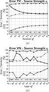 |
Figure 8. Evolution of reconstruction quality metrics over iterations/layers t for the intermediate estimates qt provided by (a) TV and (b) VN. |
 |
Figure 9. Intermediate equivalent source reconstructions qt of the baffled circular piston in Figure 3b vibrating at f=1 kHz. The top row (a–f) shows estimates provided by TV after (a) t=1, (b) t=5, (c) t=10, (d) t=50, (e) t=100, and (f) t=500 iterations. The bottom row (g–l) shows estimates provided by the even layers of the VN, where (g) is the initial approximation q0 according to equation (31), and (l) is the final network output q10. |
What is more, for most neural networks with latent hidden layers, whose dimensionality may vastly differ, only the initial input and the final output are expressed in interpretable domains. Consequently, they typically require specialized interpretative tools, such as Grad-CAM [47], to visualize the contribution of individual layers to the model output. In contrast, the manifest intermediate representations  of the VN all share the same N-dimensional domain as the ground truth
  , which inherently allows the computation of normalized spatial difference maps
 ![Mathematical equation: $ {{\mathbf {e}}}^t=[e^t_0, e^t_1, \ldots , e^t_N]^T \in {\mathbb {R}}^N $](/articles/aacus/full_html/2025/01/aacus240143/aacus240143-eq190.gif) whose elements
whose elements
 (38)
(38)
describe the normalized squared deviation in source strength magnitude between the elements  of particular layer outputs qt and the corresponding elements qn,ref of a target reference qref, which can be visualized as heatmaps. This not only allows to spatially determine the reconstruction accuracy of intermediate estimates qt by comparing them to the ground truth reference qref=qtrue as shown in Figures 10a–10f, but also to specify in detail where and how each layer (or groups of layers) spatially alters the equivalent source distribution by comparing its input qref=qt−1 to its output qt as shown in Figures 10g–10l.
 |
Figure 10. Spatial difference maps et of the VN according to equation (38) for the baffled circular piston in Figure 3b vibrating at f=1 kHz. The top row (a–f) shows the spatial difference between the even VN layer outputs qt of Figure 9(g–l) and the ground truth reference qref=qtrue in Figure 3b. The bottom row (g–l) shows the spatial difference between curated VN layer outputs qt and their respective layer inputs qref=qt−1. |
As expected, TV shows progressive improvement of accuracy over iterations qt in Figures 9a–9f and 8a by repeatedly reducing the model mismatch while ensuring a piecewise-constant appearance trough sparse spatial gradients in each iteration step t. However, final convergence to an optimal solution typically requires thousands of iterations as improvements get smaller over time, as can be seen in Figure 8a.
In contrast, the VN is merely trained to provide an accurate final output q10 for a wide range of problem setups, while intermediate predictions qt for 0≤t≤9 just serve as means to this end and are thus free to vary to ensure generalization and robustness. While training is expensive and time consuming, it needs to be done only once in advance of the actual retrieval tasks, which are then performed much faster with the trained VN compared to traditional iterative approaches like TV.
While the final output q10 of the VN in Figure 9l (also depicted larger in Fig. 5f) closely matches the ground truth qtrue in Figure 3b, reconstruction accuracy greatly fluctuates across the intermediate VN layers, as can be seen in Figures 9g–9l and 10a–10f, as well as Figure 8b. Despite a fairly accurate initial approximation q0 in Figure 9g according to equation (31), and the layer-wise loss function in equation (32) that guides the intermediate layer outputs qt to match the ground truth qtrue in the early phase of training, the VN does not progressively improve upon its initializer across layers, but rather modifies it in unexpected ways:
The data-driven continuation of the TSVD q0 of equation (31) yields only a minor improvement over the traditional TSVD solution qTSVD of equation (13) as seen in Figure 8b by adding neurally modified source and field modes that correspond to the left and right singular vectors ui and vi of the truncated singular values  , respectively. These reintroduced higher-order singular values are associated to modal patterns of higher wavenumber (representing evanescent waves) which add subtle structural details to the truncated approximation qTSVD, as best seen in Figure 10g.
In the early VN layers qt with 0≤t≤3, the noisy artifacts and side lobes in the periphery of the piston are greatly magnified, along with the general source strengths, as represented by Figures 9g, 9h and 10a, 10b, 10g, 10h, which yields a large increase in RMSE and a drop in PSNR in Figure 8b. However, the area of the piston structurally remains almost the same for those early layers and apparently changes almost only in its spatial extent.
In the middle layers qt with 4≤t≤7, the VN starts to locally change the structure of the piston area, first increasing its center gap in Figure 9i, then closing it at the expense of introducing a ring-like ripple in Figure 9j, which is ultimately flattened to an almost constant surface level. In those middle layers, the noisy artifacts at the baffle become successively more fine-grained and are alternately suppressed (odd layers, not shown for brevity) and enhanced (even layers), which is reflected by the error fluctuations in Figure 8b.
The last layers qt with 8≤t≤10 largely focus on gradually suppressing the remaining noise at the baffle, and reducing the error on the piston's border by fitting its spatial extension and making it more sharp-edged. Here, changes on the piston area are rather superficial and do not substantially alter its structural appearance, besides a global change in magnitude, as reflected by Figures 9k, 9l and 10e–10f, 10k, 10l. In the final layer q10 in Figure 9l, the residual noise at the baffle is fully removed and the piston is approximated with high accuracy, as seen in Figure 8b.
What strikes the attention is that successive layers either complement each other by respectively modifying diametrically opposite regions as seen in Figures 10c, 10d, 10k, 10l, or they operate on the same regions to potentiate or undo their impact as seen in Figures 10i, 10j. This becomes more apparent when also considering the odd VN layers for analysis, which, however, are not shown for brevity. Also, note that this iterative evolution is unique to the piston example, and it may be different for other vibrational patterns (as it is for the quadrupole and the plate).
One could get the impression that the VN potentially gets by (or even flourishes) with fewer than T=10 layers, as some layers obviously degrade accuracy instead of improving it, which in turn prompts subsequent layers for compensation. However, initial experiments suggest the contrary, where a reduction of network depth T<10 consistently resulted in a poorer generalization and larger prediction errors. Hence, some amount of back and forth optimization by consecutive layers may appear necessary to enable robust generalization. And it can neither be recommended to overly restrict the depth T of the VN, nor to strictly enforce progressive improvement of the holographic image across VN layers that would resemble TV in Figure 8a, e.g. by discarding the exponential weighting of the layer-wise losses in equation (32) for training.
7 Case study on array measurements
7.1 Measurement and loudspeaker setup
An experimental case study is carried out to evaluate the VN under measured real-world conditions. The device under study is a custom-made rectangular box [109] of geometry 70×60×48 cm3, equipped with multiple independently-driven loudspeakers. The two large loudspeakers are of the diameter ∅=17 cm, while the four small loudspeakers are of the diameter ∅=8 cm. The exact positions of the loudspeakers are depicted in Figure 11a. The active loudspeaker layout involves the large loudspeaker Nr. 3 and three small loudspeakers Nr. 10, 12 and 13.
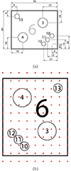 |
Figure 11. (a) Geometry and (b) microphone layout of the custom-made loudspeaker box [109]. |
Consecutive nearfield measurements of the radiated sound field were taken in an anechoic room using a planar microphone array patch, consisting of 12 sound intensity probes of type PU Mini from Microflown Technologies arranged on an equidistant 3×4 grid with an inter-microphone spacing of Δx,Δy=7.5 cm, which was positioned zm=2.5 cm above the source and was manually moved between measurements to uniformly cover the whole source. The microphone spacing results in a spatial sampling limit of f=c/(2Δx)=2286 Hz. Due to the geometrical mismatch between the box and the composite array, some of the overall Mx×My=12×9→M=108 measurement points lie outside the source domain, as shown in Figure 11b.
The impulse responses of the microphone array are determined individually for each loudspeaker by a swept sine technique [110] so that one can conveniently control the contribution of each of the 1≤l≤4 active loudspeakers to the total sound field. The impulse responses are subsequently transformed into the frequency domain by the Fourier transformation, from which only the sound pressure spectra at f=1150 Hz are considered for reconstruction.
The total monochromatic pressure field is composed as the superposition of each loudspeaker measurement as
 (39)
(39)
where |·| denotes the magnitude, and ∠· denotes the phase. The pressure measurements are normalized in magnitude such that each loudspeaker equally contributes to the overall pressure field by
 (40)
(40)
Moreover, the loudspeakers are forced to radiate approximately in phase as an attempt to minimize destructive interference of sound waves that can otherwise manifest as misplaced source estimates in the final reconstruction. This phase correction is done for each loudspeaker individually by shifting the phase of its associated pressure measurements by the negative angle of the pressure measurement of maximum magnitude to make it zero-phase as
 (41)
(41)
The magnitude- and phase-corrected measurements
 (42)
(42)
are finally used to retrieve the active loudspeaker layout on the box for the exemplary radiation frequency based on the VN and its benchmarks.
The equivalent source model of the side of the box consists of Nx×Ny=50×40→N=2000 monopoles, which are equally distributed over the size of the entire measurement surface of 82.5×60 cm2, thus partly exceeding the actual source region.
7.2 Reconstructed loudspeaker layout
Figure 12 shows the estimated equivalent source distributions of the loudspeaker layout based on the reconstruction methods under study. As the true source strength distribution on the loudspeaker cones and the boundaries of the baffle is unknown and not part of the measured data, one cannot reliably rank the methods’ accuracy in terms of objective metrics. But one can make general statements regarding localization and structural features of their estimated solutions based on the known geometry in Figure 11a. Once more, the source estimates embody the peculiar characteristics enforced by the individual regularization techniques.
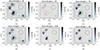 |
Figure 12. Equivalent source reconstructions of the custom-made rectangular box with loudspeakers in Figure 11 vibrating at f=1150 Hz based on (a) LN, (b) CS, (c) TV, (d) TGV, (e) PNN, and (f) VN, retrieved from real pressure measurements taken at a distance of zm=2.5 cm. Active loudspeakers are marked red. |
LN in Figure 12a shows an over-smoothed solution, where the equivalent source geometry largely exceeds the known geometry boundaries of the active loudspeakers. The spread tends to fuse neighboring loudspeakers, thereby impedes a clear separation. CS in Figure 12b produces a sparse but wrong representation of the loudspeaker layout, where loudspeakers are described by isolated monopoles, sitting on the cones and radiating with high source strength. TV in Figure 12c yields its characteristic piecewise-constant source model, where loudspeakers appear as blocky patches surrounded by staircasing artifacts. Similar to LN, TGV in Figure 12d explains the source by continuous vibrations across the baffle, but its minimum curvature constraint better confines the spread around the origins of the sound and hereby improves localization. PNN in Figure 12e inherits the characteristics of LN and approximates the loudspeakers as smooth patches, but combats over-smoothness by sparsifying the solution, which restricts active sources to the immediate vicinity of the reference positions and hereby advances localization. VN in Figure 12f provides the best estimate of the loudspeakers described by smooth but localized source strengths, with the peak magnitude centered around the origins of the sound.
All source estimates are contaminated by different degrees of side lobes and erroneous artifacts distributed over the speaker baffle. These artifacts are partly noise-induced, and in part due to the closely positioned microphones capturing structure-borne vibrations on the baffle that are inevitably excited by the motion of the loudspeaker cones, as well as by the resulting pressure fluctuations in the speaker cavity. In fact, measurement distances very close to the source may even reveal the exact microphone positions in the retrieved source strength estimates, which manifest as overactive equivalent sources. This effect is most apparent for CS in Figure 12b (although also perceivable for other methods), where ghost sources are almost regularly distributed according to the used measurement layout. These local boosts in source strength are presumably due to divisions by very small denominators in some Green's functions of the propagator in equation (2), where the distance between the associated equivalent source and measurement point approaches zero. The distance is smallest where equivalent sources and microphones align along the normal to the measurement plane, explaining the localized peaks at the microphone positions. Obviously, this boost is more pronounced for low frequencies, which further diminish the Green's functions denominators. These observations can be reproduced by simulations, showing that the reconstruction error as a function of measurement distance is a U-shaped curve, which counterintuitively increases towards closer distances.
While CS in Figure 12b suffers most from the aforementioned localized artifacts, LN in Figure 12a attenuates them by smoothing, which causes the fusion of closely neighboring source activity, impeding clear separation. For TV in Figure 12c and TGV in Figure 12d, artifacts appear more finely grained and pronounced, making it difficult to distinguish the actual loudspeakers from spurious ghost sources. Moreover, these convolutional approaches induce transient boundary effects by enhancing local source strength near the confining edges of the source model, which are most prominent at the bottom edge. The PNN in Figure 12e and the VN in Figure 12f both suppress noisy artifacts on the baffle most significantly. While the PNN relies on an explicit spatial sparsity constraint to limit non-zero source strengths, the VN implicitly filters out noise by constraining the solution in different domains based on generalized transformations, which enables a more precise spatial allocation of active sources at the reference positions. Even though the convolutional layers of VN are prescribed with the same boundary conditions as TV and TGV, boundary effects are largely compensated, which makes VN again stand out in terms of robustness against errors of these kinds.
One more aspect affecting all handcrafted reconstruction methods in Figures 12a–12d is the offset between the true and the estimated centers of the loudspeakers, which negatively impacts their localization and is most pronounced for the upper left loudspeaker. The reasons for this offset are twofold: First, unfavourable phase relations between the individual loudspeakers may cause con-/destructive interferences of the radiated sound waves, yielding local sound pressure deviations that can eventually lead to misplacements in the reconstructed source distribution. Although the in-phase correction of the loudspeakers in equation (41) alleviates the offset, it cannot eliminate it entirely, which indicates yet another contributing factor. A small geometrical mismatch between the true measurement positions and the ideal equidistant model grid may be introduced by the imperfect manual repositioning of the microphone array patch over the source domain. As the exact measurement positions are not accessible, this mismatch cannot be compensated for and needs to be accepted. While the handcrafted approaches in Figures 12a–12d fail to cope with these imperfections, the learned PNN in Figure 12e can partly mitigate their impact by relocating the equivalent sources to locally alter sound wave interference, which alleviates the offset e.g. for the loudspeaker in the upper left. However, there still remains a substantial mismatch in true and estimated spatial extent. The learned VN in Figure 12f concentrates the source strength near the centers of the loudspeakers and thereby fully removes the offset. This type of offset is taken into account during training by superimposing simple sources with random phase relations, which simulates the attenuating/amplifying effects of wave interference on the measurement snapshots, causing local shifts in sound pressure. In this way, a single magnitude source distribution can be linked to a multitude of measurements with varying degrees of local offsets. By jointly matching the source magnitude and complex components during training, the network is incentivized to compensate for such offsets in the input measurements to infer the related singular ground truth. Note that one could further improve robustness by simulating array imperfections, such as imprecise gain matching or inexact positioning of microphones during data pair generation, which is, however, not considered in this study.
In summary, VN in Figure 12f seems to be robust to the measurement noise and array imperfections in contrast to its benchmarks, as it effectively suppresses erroneous side lobes and artifacts, yielding a nearly source-free background with only nuanced activation at the speaker baffle. The estimated source strengths are concentrated and well-localized at the actual loudspeaker locations. Apparently, the performance of VN stays accurate and reliable under real-world conditions, despite its training exclusively considered simulated and simple data, which underlines its preferable generalizability and makes its application to NAH problems appealing.
8 Conclusion
This paper proposed a Variational Network to solve the planar nearfield acoustic holography problem, which is generally ill-posed. The Variational Network is a physics-constrained neural network based on an early-stopped and unrolled iterative optimizer, which was trained on generic simulated data. The proposed network was compared with a variety of regularized solutions from the seminal literature and a more recent physics-informed neural approach, and generally outperformed all of them.
The largest part of our assessment study focused on a simulation study to evaluate the methods’ responses to different source characteristics. Each of the simulated source patterns, comprised of a center-driven plate, a baffled piston, and a quadrupole, represented a different acoustical phenomenon, including smooth surface vibration, in-phase displacement and spatial sparsity.
The study revealed that the established solvers, as well as the physics-informed neural benchmark, heavily relied on appropriate task-specific knowledge and required careful tuning of regularization parameters to achieve optimal results, and yet their success was bound to certain source characteristics. In contrast, the Variational Network generalized remarkably well to different source characteristics without the need for human intervention, as it based its predictions not only on prior acoustical knowledge, but also on learned information about the generic data it was trained on. Surprisingly, even source characteristics that were not explicitly trained for were faithfully retrieved.
The Variational Network was also applied for wide-band reconstruction of the simulated piston and its associated acoustic field and it provided accurate results within reasonable errors far beyond the spatial sampling limit, where all except one of the conventional methods failed. Even though the network exploits a least norm approximation of the target source as initial input, it reliably suppressed its inherent under-sampling artifacts up to frequencies twice the spatial sampling limit.
The reconstruction performance of the network was validated experimentally under real-world conditions using available sound pressure measurements of a dispersed loudspeaker distribution with known geometry. Compared with the established solvers and the neural benchmark, the Variational Network turned out more robust to the measurement noise and array imperfection, as it showed superior source localization and separation, and it suppressed erroneous artifacts most reliably. Moreover, the proposed method was the only investigated method capable of handling unfavorable phase relations between the individual loudspeakers without introducing an offset between the estimated and target source positions. This ability was attributed to the use of superimposed sources with random phase relations during training, which linked measurements with different patterns of wave interference to the same magnitude source distribution.
Moreover, the structural similarity of the Variational Network to familiar iterative solvers makes its predictions more transparent and explainable compared to black-box neural networks. This allowed to analyze the estimated holographic image as it evolves across the network layers/iterations for the piston example, providing insights into the network's decision-making without relying on specialized interpretative tools.
Successful reconstruction of sparse source patterns required special attention. Convolutional layers of the Variational Network naturally tend to enhance spatially smooth and extended structures, so that delivering structurally sparse outputs instead would require a considerable amount of training under a naive loss. Rather than refining the focus of a few non-zero source strengths to the correct locations, the network would learn to produce zeros as trivial output, from which it would struggle to recover. Adding the normalized cross correlation as an auxiliary loss function to enforce structural similarity, regardless of scaling and bias errors, was key. Even in the early stages of training, this successfully prevented trivial network outputs.
Taking all of the above into account, the proposed method was found to be well suited to the wide-band reconstruction of a variety of planar source patterns and their radiated acoustic nearfield from ill-posed measurements, without the need for any fine-tuning of the parameters. It was also found that the method could operate reliably under both simulated and real-world conditions. Although the network was evaluated using fairly simple source configurations, these differed greatly in character and were nowhere near as complex as the training data. Nevertheless, the training data was predicted with high accuracy, offering hope that the network can accurately resolve more challenging vibrating surfaces, such as the soundboards of musical instruments. This remains subject of further investigation.
Acknowledgments
Funding
The authors received no funding to complete this research.
Conflicts of interest
The authors declare no conflict of interest.
Data availability statement
The research data associated with this article are available in https://github.com/manuelpagavino/nah-variational-network, under the reference https://doi.org/10.5281/zenodo.15852281.
References
- J. Maynard, E. Williams, Y. Lee: Nearfield acoustic holography: I. Theory of generalized holography and the development of NAH. The Journal of the Acoustical Society of America 78 (1985) 1395–1413 [Google Scholar]
- H. Fleischer: Fourier-Akustik: Beschreibung der Schallstrahlung von ebenen Schwingern mit Hilfe der räumlichen Fourier-Methode. VDI Verlag Düsseldorf, 1988 [Google Scholar]
- J. Hald: Basic theory and properties of statistically optimized near-field acoustical holography. The Journal of the Acoustical Society of America 125, 05 (2009) 2105–2120 [Google Scholar]
- Z. Wang, S. Wu: Helmholtz equation-least-squares method for reconstructing acoustic pressure field. The Journal of the Acoustical Society of America 102, 10 (1997) 2020–2032 [Google Scholar]
- A. Sarkissian: Method of superposition applied to patch near-field acoustic holography. The Journal of the Acoustical Society of America 118, 08 (2005) 671–678 [Google Scholar]
- W.A. Veronesi, J.D. Maynard: Digital holographic reconstruction of sources with arbitrarily shaped surfaces. The Journal of the Acoustical Society of America 85, 2 (1989) 588–598 [Google Scholar]
- B.-K. Kim, J. Ih: On the reconstruction of the vibro-acoustic field over the surface enclosing an interior space using the boundary element method. The Journal of the Acoustical Society of America 100, 11 (1996) 3003–3016 [Google Scholar]
- A. Schuhmacher, J. Hald, K. Rasmussen, P.C. Hansen: Sound source reconstruction using inverse boundary element calculations. The Journal of the Acoustical Society of America 113, 01 (2003) 114–127 [CrossRef] [PubMed] [Google Scholar]
- N. Valdivia, E. Williams: Implicit methods of solution to integral formulations in boundary element method based nearfield acoustic holography. The Journal of the Acoustical Society of America 116, 09 (2004) 1559–1572 [Google Scholar]
- P. Hansen: Rank-Deficient and Discrete Ill-Posed Problems: Numerical Aspects of Linear Inversion. SIAM Monographs of Mathematical Modeling and Computation, Society for Industrial and Applied Mathematics, 1987 [Google Scholar]
- G.H. Golub, P.C. Hansen, D.P. O`Leary: Tikhonov regularization and total least squares. SIAM Journal on Matrix Analysis and Applications 21 (1999) 185–194 [Google Scholar]
- M. Elad: Sparse and Redundant Representations – From Theory to Applications in Signal and Image Processing. Springer, 2010 [Google Scholar]
- E.J. Candès, M.B. Wakin: An introduction to compressive sampling. IEEE Signal Processing Magazine 25, 2 (2008) 21–30 [Google Scholar]
- S. Foucart, H. Rauhut: A mathematical introduction to compressive sensing, in: Applied and Numerical Harmonic Analysis. Birkhäuser New York, 2013 [Google Scholar]
- H. Boche, R. Calderbank, G. Kutyniok, J. Vybíral, Eds.: Compressed sensing and its applications, in: Applied and Numerical Harmonic Analysis. Birkhäuser Cham, 2015 [Google Scholar]
- D. Donoho: Compressed sensing. IEEE Transactions on Information Theory 52, 4 (2006) 1289–1306 [CrossRef] [MathSciNet] [Google Scholar]
- S. Gade, J. Hald, K. Ginn: Wideband acoustical holography. Sound and Vibration Magazine 50, 04 (2016) 8–13 [Google Scholar]
- D.-Y. Hu, H.-B. Li, Y. Hu, Y. Fang: Sound field reconstruction with sparse sampling and the equivalent source method. Mechanical Systems and Signal Processing 108, 08 (2018) 317–325 [Google Scholar]
- C.-X. Bi, Y. Liu, L. Xu, Y.-B. Zhang: Sound field reconstruction using compressed modal equivalent point source method. The Journal of the Acoustical Society of America 141, 01 (2017) 73–79 [Google Scholar]
- N.M. Abusag, D.J. Chappell: On sparse reconstructions in near-field acoustic holography using the method of superposition. Journal of Computational Acoustics 24, 09 (2016) 1650009 [Google Scholar]
- G. Chardon, L. Daudet, A. Peillot, F. Ollivier, N. Bertin, R. Gribonval: Near-field acoustic holography using sparse regularization and compressive sampling principles. The Journal of the Acoustical Society of America 132, 09 (2012) 1521–1534 [CrossRef] [PubMed] [Google Scholar]
- J. Hald: Fast wideband acoustical holography. The Journal of the Acoustical Society of America 139, 04 (2016) 1508–1517 [Google Scholar]
- C.-X. Bi, Y. Liu, Y.-B. Zhang, L. Xu: Sound field reconstruction using inverse boundary element method and sparse regularization. The Journal of the Acoustical Society of America 145, 05 (2019) 3154–3162 [Google Scholar]
- C.-X. Bi, Y. Liu, Y.-B. Zhang, L. Xu: Extension of sound field separation technique based on the equivalent source method in a sparsity framework. Journal of Sound and Vibration 442, 03 (2019) 125–137 [Google Scholar]
- E. Fernandez-Grande, L. Daudet: Compressive acoustic holography with block-sparse regularization. The Journal of the Acoustical Society of America 143, 06 (2018) 3737–3746 [CrossRef] [PubMed] [Google Scholar]
- J. Liu, Y. Liu, J.S. Bolton: Acoustic source reconstruction and visualization based on acoustic radiation modes. Journal of Sound and Vibration 437, 09 (2018) 358–372 [Google Scholar]
- E. Fernandez-Grande, A. Xenaki, P. Gerstoft: A sparse equivalent source method for near-field acoustic holography. The Journal of the Acoustical Society of America 141, 01 (2017) 532–542 [CrossRef] [PubMed] [Google Scholar]
- Y. He, L. Chen, Z. Xu, Z. Zhang: A compressed equivalent source method based on equivalent redundant dictionary for sound field reconstruction. Applied Sciences 9, 02 (2019) 808 [Google Scholar]
- J. Hald: A comparison of iterative sparse equivalent source methods for near-field acoustical holography. The Journal of the Acoustical Society of America 143, 06 (2018) 3758–3769 [CrossRef] [PubMed] [Google Scholar]
- Y.-B. Zhao: Sparse Optimization Theory and Methods, 1 edn. CRC Press, 2018 [Google Scholar]
- M.R. Bai, J.-H. Lin, K.-L. Liu: Optimized microphone deployment for near-field acoustic holography: to be, or not to be random, that is the question. Journal of Sound and Vibration 329, 07 (2010) 2809–2824 [Google Scholar]
- Y. Liu, C.-X. Bi, L. Xu, Y.-B. Zhang: Sound field reconstruction using equivalent source method based on a redundant dictionary, in: INTER-NOISE and NOISE-CON Congress and Conference Proceedings. Institute of Noise Control Engineering, 2017, pp. 1996–2998 [Google Scholar]
- M. Pagavino: Derivative-based regularization of inverse problems in acoustic holography. Master's thesis, University of Music and Performing Arts Graz – Institute of Electronic Music and Acoustics, 2019 [Google Scholar]
- I. Goodfellow, Y. Bengio, A. Courville: Deep Learning. MIT Press, 2016. http://www.deeplearningbook.org [Google Scholar]
- L. Xu, J. Ren, C. Liu, J. Jia: Deep convolutional neural network for image deconvolution. Advances in Neural Information Processing Systems 2, 01 (2014) 1790–1798 [Google Scholar]
- O. Kupyn, V. Budzan, M. Mykhailych, D. Mishkin, J. Matas: DeblurGAN: blind motion deblurring using conditional adversarial networks, in: 2018 IEEE/CVF Conference on Computer Vision and Pattern Recognition, 2018 [Google Scholar]
- J. Xie, L. Xu, E. Chen: Image denoising and inpainting with deep neural networks, in: Advances in Neural Information Processing Systems 25, 2012 [Google Scholar]
- C. Dong, C.C. Loy, K. He, X. Tang: Image super-resolution using deep convolutional networks. IEEE Transactions on Pattern Analysis and Machine Intelligence 38, 06 (2015) 295–307 [Google Scholar]
- M. Duarte, M. Davenport, D. Takhar, J. Laska, T. Sun, K. Kelly, R. Baraniuk: Single-pixel imaging via compressive sampling. IEEE Signal Processing Magazine 25, 04 (2008) 83–91 [Google Scholar]
- E. Candès, J. Romberg, T. Tao: Stable signal recovery from incomplete and inaccurate measurements. Communications on Pure and Applied Mathematics 59, 08 (2006) 1207–1223 [CrossRef] [Google Scholar]
- M. Olivieri, M. Pezzoli, R. Malvermi, F. Antonacci, A. Sarti: Near-field acoustic holography analysis with convolutional neural networks, in: INTER-NOISE and NOISE-CON Congress and Conference Proceedings, Seoul, Korea, August 2020. Institute of Noise Control Engineering, Vol. 261 (2020) 5607–5618 [Google Scholar]
- M. Olivieri, M. Pezzoli, F. Antonacci, A. Sarti: Near field acoustic holography on arbitrary shapes using convolutional neural network, in: 2021 29th European Signal Processing Conference (EUSIPCO), 2021, pp. 121–125 [Google Scholar]
- J. Wang, Z. Zhang, Y. Huang, Z. Li, Q. Huang: A 3D convolutional neural network based near-field acoustical holography method with sparse sampling rate on measuring surface. Measurement 177 (2021) 109297 [Google Scholar]
- J. Wang, Z. Zhang, Z. Li, Q. Huang: Research on joint training strategy for 3D convolutional neural network based near-field acoustical holography with optimized hyperparameters. Measurement 202 (2022) 111790 [Google Scholar]
- J. Wang, W. Zhang, Z. Zhang, Y. Huang: A cylindrical near-field acoustical holography method based on cylindrical translation window expansion and an autoencoder stacked with 3D-CNN layers. Sensors 23, 04 (2023) 4146 [Google Scholar]
- Z. Cao, L. Geng, J. Wang: Sparse-sampled near-field acoustic holography based on 3D-CNN and dense block, in: 2024 7th International Conference on Information Communication and Signal Processing (ICICSP), 2024, pp. 483–487 [Google Scholar]
- H. Kafri, M. Olivieri, F. Antonacci, M. Moradi, A. Sarti, S. Gannot: Grad-cam-inspired interpretation of nearfield acoustic holography using physics-informed explainable neural network, in: ICASSP 2023 – 2023 IEEE International Conference on Acoustics, Speech and Signal Processing (ICASSP), 2023, pp. 1–5 [Google Scholar]
- S. Koyama, J.G.C. Ribeiro, T. Nakamura, N. Ueno, M. Pezzoli: Physics-informed machine learning for sound field estimation: fundamentals, state of the art, and challenges. IEEE Signal Processing Magazine 41, 6, (2024) 60–71 [Google Scholar]
- X. Karakonstantis, E. Fernandez-Grande: Generative adversarial networks with physical sound field priors. The Journal of the Acoustical Society of America 154, 08 (2023) 1226–1238 [Google Scholar]
- T. Lobato, R. Sottek, M. Vorländer: Using learned priors to regularize the helmholtz equation least-squares method. The Journal of the Acoustical Society of America 155, 02 (2024) 971–983 [Google Scholar]
- S. Chaitanya, S. Sriraman, S. Srinivasan, K. Srinivasan: Machine learning aided near-field acoustic holography based on equivalent source method. The Journal of the Acoustical Society of America 153, 2 (2023) 940 [Google Scholar]
- G. Karniadakis, Y. Kevrekidis, L. Lu, P. Perdikaris, S. Wang, L. Yang: Physics-informed machine learning. Nature Reviews Physics 3, 6 (2021) 422–440 [Google Scholar]
- M. Raissi, P. Perdikaris, G. Karniadakis: Physics-informed neural networks: a deep learning framework for solving forward and inverse problems involving nonlinear partial differential equations. Journal of Computational Physics 378 (2019) 686–707 [CrossRef] [Google Scholar]
- H. Bi, T. Abhayapala: Point neuron learning: a new physics-informed neural network architecture. EURASIP Journal on Audio, Speech, and Music Processing 2024, 1, (2024) 56 [Google Scholar]
- F.A. Marco Olivieri, M. Pezzoli, A. Sarti: A physics-informed neural network approach for nearfield acoustic holography. Sensors, 21, 23 (2021) 7834 [Google Scholar]
- X. Luan, M. Olivieri, M. Pezzoli, F. Antonacci, A. Sarti: Complex – valued physics-informed neural network for near-field acoustic holography, in: 2024 32nd European Signal Processing Conference (EUSIPCO), 2024, pp. 126–130 [Google Scholar]
- M. Olivieri, X. Karakonstantis, M. Pezzoli, F. Antonacci, A. Sarti, E. Fernandez-Grande: Physics-informed neural network for volumetric sound field reconstruction of speech signals. EURASIP Journal on Audio, Speech, and Music Processing 2024, 1 (2024) 42 [Google Scholar]
- X. Karakonstantis, D. Caviedes Nozal, A. Richard, E. Fernandez-Grande: Room impulse response reconstruction with physics-informed deep learning. The Journal of the Acoustical Society of America 155, 02 (2024) 1048–1059 [Google Scholar]
- X. Chen, F. Ma, A. Bastine, P. Samarasinghe, H. Sun: Sound field estimation around a rigid sphere with physics-informed neural network, in: 2023 Asia Pacific Signal and Information Processing Association Annual Summit and Conference (APSIPA ASC), 2023, pp. 1984–1989 [Google Scholar]
- F. Ma, S. Zhao, I.S. Burnett: Sound field reconstruction using a compact acoustics-informed neural network. The Journal of the Acoustical Society of America 156, 09 (2024) 2009–2021 [Google Scholar]
- J. Ribeiro, S. Koyama, R. Horiuchi, H. Saruwatari: Sound field estimation based on physics-constrained kernel interpolation adapted to environment. IEEE/ACM Transactions on Audio, Speech, and Language Processing PP, 01 (2024) 1–16 [Google Scholar]
- K. Shigemi, S. Koyama, T. Nakamura, H. Saruwatari: Physics-informed convolutional neural network with bicubic spline interpolation for sound field estimation, in: 2022 International Workshop on Acoustic Signal Enhancement (IWAENC), 2022, pp. 1–5 [Google Scholar]
- E. Kobler, T. Klatzer, K. Hammernik, T. Pock: Variational networks: connecting variational methods and deep learning, in: Pattern Recognition. GCPR 2017, Germany. Springer, 2017, pp. 281–293 [Google Scholar]
- K. Hammernik, T. Klatzer, E. Kobler, M.P. Recht, D.K. Sodickson, T. Pock, F. Knoll: Learning a variational network for reconstruction of accelerated MRI data. Magnetic Resonance in Medicine 79, 11 (2017) 3055–3071 [Google Scholar]
- Y. Chen, W. Yu, T. Pock: On learning optimized reaction diffusion processes for effective image restoration, in: 2015 IEEE Conference on Computer Vision and Pattern Recognition (CVPR), 2015, pp. 5261–5269 [Google Scholar]
- Y. Chen, T. Pock: Trainable nonlinear reaction diffusion: a flexible framework for fast and effective image restoration. IEEE Transactions on Pattern Analysis and Machine Intelligence 39 (2016) 1256–1272 [Google Scholar]
- H. Chen, Y. Zhang, Y. Chen, J. Zhang, W. Zhang, H. Sun, Y. Lv, P. Liao, J. Zhou, G. Wang: LEARN: learned experts’ assessment-based reconstruction network for sparse-data CT. IEEE Transactions on Medical Imaging 37, 6 (2018) 1333–1347 [Google Scholar]
- S. Roth, M.J. Black: Fields of experts. International Journal of Computer Vision 82, 04 (2009) 205–229 [Google Scholar]
- T. Klatzer, K. Hammernik, P. Knobelreiter, T. Pock: Learning joint demosaicing and denoising based on sequential energy minimization, in: 2016 IEEE International Conference on Computational Photography (ICCP), (Evanston, IL, USA). IEEE, 2016, pp. 1–11 [Google Scholar]
- A. Hirose: Complex-Valued Neural Networks. Vol. 32. Springer, 2006 [Google Scholar]
- J.B. Mingsian, R. Bai, J.-G. Ih: Nearfield Array Signal Processing Algorithms. John Wiley & Sons, Ltd, 2013 [Google Scholar]
- M. Hanke, A. Neubauer, O. Scherzer: A convergence analysis of the landweber iteration for nonlinear ill-posed problems. Numerische Mathematik 72 (1995) 21–37 [Google Scholar]
- M. Benzi: Preconditioning techniques for large linear systems: a survey. Journal of Computational Physics 182 (2002) 418–477 [Google Scholar]
- L. Rudin, S. Osher, E. Fatemi: Nonlinear total variation based noise removal algorithms. Physica D: Nonlinear Phenomena 60 (1992) 259–268 [NASA ADS] [CrossRef] [MathSciNet] [Google Scholar]
- K. Bredies, K. Kunisch, T. Pock: Total Generalized Variation. SIAM Journal on Imaging Sciences 3, 3, (2010) 492–526 [CrossRef] [MathSciNet] [Google Scholar]
- V. Vishnevskiy, J. Walheim, S. Kozerke: Deep variational network for rapid 4D flow MRI reconstruction. Nature Machine Intelligence 2, 4 (2020) 228–235 [Google Scholar]
- V. Vishnevskiy, R. Rau, O. Goksel: Deep variational networks with exponential weighting for learning computed tomography, in: Medical Image Computing and Computer Assisted InterventionMICCAI 2019: 22nd International Conference, Shenzhen, China, October 13–17, 2019, Proceedings, Part VI 22. Springer International Publishing, 2019, pp. 310–318 [Google Scholar]
- V. Vishnevskiy, S.J. Sanabria, O. Goksel: Image reconstruction via variational network for real-time hand-held sound-speed imaging, in: Machine Learning for Medical Image Reconstruction: First International Workshop, MLMIR 2018, Held in Conjunction with MICCAI 2018, Granada, Spain, September 16, 2018, Proceedings 1. Springer International Publishing, 2018, pp. 120–128 [Google Scholar]
- D. Gilton, G. Ongie, R. Willett: Neumann networks for linear inverse problems in imaging. IEEE Transactions on Computational Imaging 6 (2020) 328–343 [Google Scholar]
- J. Adler, O. Öktem: Solving ill-posed inverse problems using iterative deep neural networks. Inverse Problems 33 (2017) 124007 [Google Scholar]
- J. Xiang, Y. Dong, Y. Yang: FISTA-Net: learning a fast iterative shrinkage thresholding network for inverse problems in imaging. IEEE Transactions on Medical Imaging 40, 01 (2021) 1329–1339 [Google Scholar]
- G. Nakerst, J. Brennan, M. Haque: Gradient descent with momentum – to accelerate or to super-accelerate? arXiv:2001.06472, (2020) [Google Scholar]
- L. Condat: A primal-dual splitting method for convex optimization involving lipschitzian, proximable and linear composite terms. Journal of Optimization Theory and Applications 158, 2 (2013) 460–479 [Google Scholar]
- B. Vu: A splitting algorithm for dual monotone inclusions involving cocoercive operators. Advances in Computational Mathematics 38, 04 (2011) 667–681 [Google Scholar]
- A. Chambolle, T. Pock: A first-order primal-dual algorithm for convex problems with applications to imaging. Journal of Mathematical Imaging and Vision 40, 05 (2011) 120–145 [NASA ADS] [CrossRef] [Google Scholar]
- K. Hammernik: Variational networks for medical image reconstruction. PhD thesis, Technical University of Graz – Institute of Computer Graphics and Vision, 2019 [Google Scholar]
- N. Guberman: On complex valued convolutional neural networks. arXiv:1602.09046, (2016) [Google Scholar]
- S. Chen, S. McLaughlin, B. Mulgrew: Complex-valued radial basic function network, part I: Network architecture and learning algorithms. Signal Processing 35, 1 (1994) 19–31 [Google Scholar]
- S. Ramasamy, S. Sundaram, N. Sundararajan: A fully complex-valued radial basis function network and its learning algorithm. International Journal of Neural Systems 19, 08 (2009) 253–267 [Google Scholar]
- D. Caviedes-Nozal, N.A.B. Riis, F.M. Heuchel, J. Brunskog, P. Gerstoft, E. Fernandez-Grande: Gaussian processes for sound field reconstruction. The Journal of the Acoustical Society of America 149, 02 (2021) 1107–1119 [Google Scholar]
- I. Steinwart, A. Christmann: Support vector machines, in: Information Science and Statistics. Springer New York, New York, NY, 2008 [Google Scholar]
- S. Ioffe, C. Szegedy: Batch normalization: accelerating deep network training by reducing internal covariate shift. arXiv:1502.03167, (2015) [Google Scholar]
- D. Ulyanov, A. Vedaldi, V. Lempitsky: Instance normalization: the missing ingredient for fast stylization. arXiv:1607.08022, (2016) [Google Scholar]
- C. Trabelsi, O. Bilaniuk, Y. Zhang, D. Serdyuk, S. Subramanian, J.F. Santos, S. Mehri, N. Rostamzadeh, Y. Bengio, C.J. Pal: Deep complex networks. arXiv:1705.09792, (2017) [Google Scholar]
- J.S. Dramsch, M. Lüthje, A.N. Christensen: Complex-valued neural networks for machine learning on non-stationary physical data. Computers and Geosciences 146, 01 (2021) 104643 [Google Scholar]
- H. Vogel: A better way to construct the sunflower head. Mathematical Biosciences 44, 3 (1979) 179–189 [Google Scholar]
- N. Benoudjit, M. Verleysen: On the kernel widths in radial-basis function networks. Neural Processing Letters 18, 10 (2003) 139–154 [Google Scholar]
- J. Schwab, S. Antholzer, M. Haltmeier: Big in Japan: regularizing networks for solving inverse problems. Journal of Mathematical Imaging and Vision 62, 12 (2018) 445–455 [Google Scholar]
- R. Heckel: Regularizing linear inverse problems with convolutional neural networks. arXiv:1907.03100, (2019) [Google Scholar]
- D. Ulyanov, A. Vedaldi, V. Lempitsky: Deep image prior. International Journal of Computer Vision 128, 03 (2020) 1867–1888 [Google Scholar]
- D.V. Veen, A. Jalal, M. Soltanolkotabi, E. Price, S. Vishwanath, A.G. Dimakis: Compressed sensing with deep image prior and learned regularization. arXiv:1806.06438, (2018) [Google Scholar]
- H. Gupta, K.H. Jin, H.Q. Nguyen, M.T. McCann, M. Unser: CNN-based projected gradient descent for consistent CT image reconstruction. IEEE Transactions on Medical Imaging 37 (2018) 1440–1453 [Google Scholar]
- G. Mataev, M. Elad, P. Milanfar: DeepRED: deep image prior powered by RED, in: Proceedings of the IEEE/CVF International Conference on Computer Vision Workshops, 2019 [Google Scholar]
- S. Dittmer, T. Kluth, P. Maass, D. Otero Baguer: Regularization by architecture: a deep prior approach for inverse problems. Journal of Mathematical Imaging and Vision 62 (2020) 456–470 [Google Scholar]
- Z. Cheng, M. Gadelha, S. Maji, D. Sheldon: A bayesian perspective on the deep image prior, in: Proceedings of the IEEE/CVF Conference on Computer Vision and Pattern Recognition, 2019, pp. 5443–5451 [Google Scholar]
- A. Sagel, A. Roumy, C. Guillemot: Sub-dip: Optimization on a subspace with deep image prior regularization and application to superresolution, in: ICASSP 2020 – 2020 IEEE International Conference on Acoustics, Speech and Signal Processing (ICASSP), 2020, pp. 2513–2517 [Google Scholar]
- R. Heckel, P. Hand: Deep decoder: concise image representations from untrained non-convolutional networks. arXiv:1810.03982, (2018) [Google Scholar]
- Z. Wang, A. Bovik, H. Sheikh, E. Simoncelli: Image quality assessment: from error visibility to structural similarity. IEEE Transactions on Image Processing 13, 05 (2004) 600–612 [NASA ADS] [CrossRef] [Google Scholar]
- R. Mittmannsgruber: Leistungsbasierte Analyse von Luftschallübertragungsanteilen. Master's thesis, University of Music and Performing Arts Graz – Institute of Electronic Music and Acoustics, 2017 [Google Scholar]
- A. Farina: Simultaneous measurement of impulse response and distortion with a swept-sine technique. Journal of the Audio Engineering Society 11 (2000) [Google Scholar]
Cite this article as: Pagavino M. & Zotter F. 2025. Data-driven and physics-constrained acoustic holography based on optimizer unrolling. Acta Acustica, 9, 46. https://doi.org/10.1051/aacus/2025030.
All Tables
Number and dimensionality of the learnable complex-valued parameters of each VN layer t.
All Figures
|
Figure 1. Schematic iteration/layer representation of an unrolled gradient descent on a single model mismatch and regularization cost that forms the basis of the Variational Network (VN), showing its structural similarity to a typical residual neural network (ResNet). |
| In the text | |
|
Figure 2. (a) The Variational Network (VN) architecture corresponding to equation (18), comprised of (b) the model mismatch network defined by equation (19), (c) the regularizer network defined by equation (20), and (d) the momentum network defined by equation (21). |
| In the text | |
|
Figure 3. Ground truth equivalent source distributions for the (a) center-driven plate in Section 6.1, (b) baffled piston in Section 6.2, and (c) quadrupole in Section 6.3, that are used as references in the simulation study of Section 6. |
| In the text | |
|
Figure 4. Equivalent source reconstructions of the center-driven plate in Figure 3a vibrating at f=800 Hz based on (a) LN, (b) CS, (c) TV, (d) TGV, (e) PNN, and (f) VN, retrieved from measurements with SNR=28 dB taken at a distance of zm=6 cm. |
| In the text | |
|
Figure 5. Equivalent source reconstructions of the baffled circular piston in Figure 3b vibrating at f=1 kHz based on (a) LN, (b) CS, (c) TV, (d) TGV, (e) PNN, and (f) VN, retrieved from measurements with SNR=28 dB taken at a distance of zm=6 cm. |
| In the text | |
|
Figure 6. Ensemble-averaged ϵRMSE as in equation (36) in percent for the (a) reconstructed equivalent sources of the baffled piston, retrieved from measurements with SNR=28 dB taken at a distance of zm=6 cm, along with their radiated (b) sound pressure, (c) normal velocity, and (d) normal intensity field reconstructed at a distance of zR=3 cm, as in equations (4)–(6). The vertical line at f=2401 Hz marks the spatial sampling limit. |
| In the text | |
|
Figure 7. Equivalent source reconstructions of the longitudinal quadrupole in Figure 3c vibrating at f=3 kHz based on (a) LN, (b) CS, (c) CS-TV, (d) CS-TGV, (e) PNN, and (f) VN, retrieved from measurements with SNR=28 dB taken at a distance of zm=6 cm. CS-TV and CS-TGV use unity weight μ=1 for the spatial sparsity constraint. |
| In the text | |
|
Figure 8. Evolution of reconstruction quality metrics over iterations/layers t for the intermediate estimates qt provided by (a) TV and (b) VN. |
| In the text | |
|
Figure 9. Intermediate equivalent source reconstructions qt of the baffled circular piston in Figure 3b vibrating at f=1 kHz. The top row (a–f) shows estimates provided by TV after (a) t=1, (b) t=5, (c) t=10, (d) t=50, (e) t=100, and (f) t=500 iterations. The bottom row (g–l) shows estimates provided by the even layers of the VN, where (g) is the initial approximation q0 according to equation (31), and (l) is the final network output q10. |
| In the text | |
|
Figure 10. Spatial difference maps et of the VN according to equation (38) for the baffled circular piston in Figure 3b vibrating at f=1 kHz. The top row (a–f) shows the spatial difference between the even VN layer outputs qt of Figure 9(g–l) and the ground truth reference qref=qtrue in Figure 3b. The bottom row (g–l) shows the spatial difference between curated VN layer outputs qt and their respective layer inputs qref=qt−1. |
| In the text | |
|
Figure 11. (a) Geometry and (b) microphone layout of the custom-made loudspeaker box [109]. |
| In the text | |
|
Figure 12. Equivalent source reconstructions of the custom-made rectangular box with loudspeakers in Figure 11 vibrating at f=1150 Hz based on (a) LN, (b) CS, (c) TV, (d) TGV, (e) PNN, and (f) VN, retrieved from real pressure measurements taken at a distance of zm=2.5 cm. Active loudspeakers are marked red. |
| In the text | |
Current usage metrics show cumulative count of Article Views (full-text article views including HTML views, PDF and ePub downloads, according to the available data) and Abstracts Views on Vision4Press platform.
Data correspond to usage on the plateform after 2015. The current usage metrics is available 48-96 hours after online publication and is updated daily on week days.
Initial download of the metrics may take a while.