| Issue |
Acta Acust.
Volume 9, 2025
|
|
|---|---|---|
| Article Number | 41 | |
| Number of page(s) | 14 | |
| Section | Virtual Acoustics | |
| DOI | https://doi.org/10.1051/aacus/2025026 | |
| Published online | 16 July 2025 | |
Technical & Applied Article
Bidirectional surface scattering coefficients
Institute for Hearing Technology and Acoustics, RWTH Aachen University Aachen Germany
* Corresponding author: This email address is being protected from spambots. You need JavaScript enabled to view it.
Received:
25
March
2025
Accepted:
12
June
2025
Abstract
The prediction and modeling of sound propagation rely heavily on accurate representations of surface scattering. Traditional scattering coefficients, often based on random-incidence assumptions, fail to capture the directional dependence of sound reflections from rough surfaces. This paper introduces a methodology for determining and representing bidirectional surface scattering coefficients, moving beyond the limitations of existing Lambertian-based approaches. We propose a framework that leverages numerical simulations and physical measurements to compute bidirectional scattering coefficients from reflected sound pressure distributions with finite-size samples. The methodology is validated using a well-documented sinusoidal test surface, comparing our results with analytical solutions for infinite-size samples and former random-incidence scattering coefficient measurements. Additionally, we propose a data storage format compatible with the Spatially Oriented Format for Acoustics (SOFA) to facilitate the integration of bidirectional scattering coefficients into sound propagation models. This work provides a foundation for improved acoustic simulations in applications ranging from room acoustics to urban noise control.
Key words: Acoustic scattering / Bidirectional scattering coefficients / Scattering coefficients / Sound propagation modelling
© The Author(s), Published by EDP Sciences, 2025
 This is an Open Access article distributed under the terms of the Creative Commons Attribution License (https://creativecommons.org/licenses/by/4.0), which permits unrestricted use, distribution, and reproduction in any medium, provided the original work is properly cited.
1 Introduction
Surface scattering is a crucial component of sound propagation in indoor and outdoor environments. Hence, the prediction of scattering and its implementation in sound propagation simulation is essential. Up to now, scattering effects are typically accounted for by dividing the total reflected sound energy into a specular part and a non-specular (diffuse) part [1]. The specular reflection takes the exact angle which is created from the incidence angle, simply mirrored at the surface normal vector.
The standardized scattering coefficient corresponds to the angular average of random-incidence [1] and is represented by the Lambert distribution of scattered energy. In contrast to the scattering coefficient, the diffusion coefficient defines the uniformity of the directional pattern of the scattered sound [2, 3].
Mommertz proposed a correlation method to calculate the scattering coefficient for a specific incident angle, based on the reflection patterns of both a flat and the test surface [4]. The scattering coefficients of various angles can then be averaged using the Paris formula [5] to determine the random-incidence scattering coefficient. Several researchers have applied the correlation method to determine the scattering coefficient using various approaches, such as experimental measurements [3, 6], boundary element method (BEM) simulations [7, 8], and analytical methods [9].
However, the reliance on random-incidence and quasi-stochastic Lambertian scattering distributions presents limitations. For non-stochastic surfaces, the random-incidence scattering coefficient may not capture the scattering behavior accurately. This discrepancy is evident in Figure 1, where a scattering pattern from a periodic surface is compared with the Lambertian reflection from a stochastically rough surface when the acoustic wavelengths are small relative to the structure. Periodic surfaces scatter the sound into distinct directions which depend on the geometric surface structure periodicity [10]. However, many surfaces in acoustic environments, such as in room acoustics, urban acoustics (building facades), or other fields, are periodic in nature.
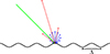 |
Figure 1. Comparison of Lambertian and real energetic sound scattering pattern. A plane wave with incidence in (green) hits a rough periodic surface (black). The reflection pattern of a sinusoidal surface (red) at Λ/λ=2 is determined after Embrechts analytical solution [7] including its direction and energy. The Lambertian model (blue) is discretized in equal angular steps of 15°. The length of the arrows represent their energies. Both reflection patterns result in a random-incident scattering coefficient of 1 as they are normalized in energy. |
Given these challenges, a method is needed to determine and represent not only stochastic but also specific bidirectional scattering phenomena more accurately. Bidirectional in this context refers to the way the sound wave scatters, capturing both incoming and outgoing directions. Such a method would improve the predictive capabilities of simulations and models that rely on scattering data, leading to better design and analysis in applications ranging from architectural acoustics to noise control, for example.
In optics, the concept of bidirectional scattering is widely applied, such as in the Bidirectional Reflectance Distribution Function (BRDF) [11]. The BRDF characterizes light reflection from a surface based on the incoming and outgoing directions. For a BRDF model to be physically accurate, it must satisfy two conditions: energy conservation and reciprocity. In acoustics, the understanding of bidirectional scattering distribution is less developed. Siltanen et al. [12] applied an acoustic BRDF to model oblique incidence in a room acoustics setting based on the random-incidence scattering coefficients due to the lack of available bidirectional scattering data.
The goal of this work is to establish a method for the determination and data representation of bidirectional scattering coefficients from reflected sound pressure distributions of finite-size samples. The method can be based on measured or numerically computed results. We aim to move beyond the limitations of random-incidence assumptions and provide a framework that accounts for the bidirectional dependence of scattering. For a proof of concept, we present a case study in which the bidirectional scattering coefficient dataset is determined from measured and simulated reflection distributions based on a surface with known bidirectional scattering properties.
2 Bidirectional scattering coefficient
The total reflected energy is equal to the incident energy multiplied by (1−α), where α is the absorption coefficient. The bidirectional scattering coefficient (sd) quantifies the portion of energy scattered in a specific direction relative to the total reflected energy. Due to the reciprocity of sound energy, the roles of the source (incident direction) and the receiver (scattered direction) can be interchanged. Mathematically, this is expressed as:
 (1)
(1)
with ϑS and φS being the incident angles and ϑR and φR being the scattering angles. The angles are defined as depicted in Figure 2. The frequency dependency is indicated by f.
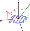 |
Figure 2. Definition of the coordinate system with the surface under investigation in blue. The incident sound direction is marked in red, where the scattered direction is marked in green. |
Similar to the random-incidence scattering coefficient, sd must satisfy the principle of energy conservation. This implies that for a given incident direction, the sum of the bidirectional scattering coefficients over all possible scattering directions or all possible source directions equals 1:
 (2)
(2)
The amount of scattered energy is influenced by the geometry and size of surface corrugations, as well as the frequency [10]. The problem is therefore scalable. To incorporate the effect of scaling, results are systematically presented using a normalized frequency axis, defined as the ratio of the structural wavelength to the sound wavelength, Λ/λ.
2.1 Determination of scattering coefficient for free-field incidence
To determine the bidirectional scattering coefficient, we first examine the process of deriving the regular scattering coefficient for free-field conditions. Following this, we will address the methodology for determining the bidirectional scattering coefficient. The correlation method [4] to determine the free-field scattering coefficient requires free-field calculations or measurements of the scattered sound pressure or reflection pattern of finite-size test samples. The following two reflection patterns must be determined:
-
p0(ϑS,φS,ϑR,φR), representing the reflection pattern of a reference flat surface with the same dimensions of the sample.
-
p1(ϑS,φS,ϑR,φR), representing the reflection pattern of the test sample.
Here, p0 serves as a reference for determining the specular reflectance. Then, the scattering coefficient for each incident plane wave direction is determined according to
 (3)
(3)
where wR is an area weighting factor resulting from the integration over the receiver half sphere, depending on the spatial distribution of sampling points.
The scattering coefficient is zero with maximum correlation between the reflection patterns p1 and p0, leading to a complete specular reflection of the surface under investigation. So, a higher correlation results in less scattering, while a lower correlation results in more scattering. Additionally, edge diffraction effects are compensated in this correlation methods, as both p0 and p1 include nearly identical edge diffraction contributions.
2.2 Definition of the bidirectional scattering coefficient
This approach can be extended towards a bidirectional scattering coefficient (sd). Firstly, the scattered energy in the specular reflection direction is determined:
 (4)
(4)
with sd being the bidirectional scattering coefficient and s is the scattering coefficient for the incident angle of (ϑS,φS). The right part of equation (4) means that the scattered energy is excluded from the total reflected energy, resulting in the energy into the specular direction. This is consistent with the application of scattering coefficients, where the total reflected energy is split into the specular part and the scattered part.
To determine sd for reflection angles other than the specular direction, the corresponding p0(ϑS,φS) have to be selected. This is achieved by taking the reference reflection pattern of the same incident angle ϑR and rotating the azimuth angle φR by π/180°. This leads to the equation (5) for sd:
 (5)
(5)
The receiver grid is determined by the resolution of the incidence angles (ϑR=ϑS), while the azimuthal angles (φR) can be chosen from user, by rotating the reference measurement p0 this can be simply done due to the rotational symmetry of the reference setup. Taking the azimuthal source resolution φS, could be a good starting point, resulting in the same source and receiver grid. Then, the source grid remains the same, while the receiver grid depends on the source grid. In other words, the receiver grid of the sound pressure is not equal to the receiver grid of the bidirectional scattering coefficient, where the source grid remains the same for both.
3 Geometry of the measurement setup
Various methods can be employed to determine the reflected sound pressure. The process begins by defining the geometric conditions.
The ISO standards 17497-1 [1] and 17497-2 [2] serve as the foundational guidelines for capturing reflected sound pressure. ISO 17497-1 specifies the requirements for the test sample, including the size and the structure of the sample and its maximum depth. ISO 17497-2 defines the measurement conditions, such as far-field criteria, the radius of the sound sources and receivers, and receiver angular resolution.
According to ISO 17497-2 [2], far-field conditions are met when the reflected sound pressure level from the test surface decreases by 6 dB for every doubling of distance, which is full-field for a receiver distance of 5 m [2]. It also suggests a maximum receiver angular resolution of 5°, leading towards the following conditions ΔϑR≤5° and ΔφR≤5°. 10 m are suggested for the source distance [2].
Embrechts et al. [13] also defined a maximal angular resolution for the receiver grid. They used the correlation method to determine the scattering coefficients from random gaussian surfaces based on an analytical approach. Hereby, they found that the angular resolution of the receiver grid should be at least
 (6)
(6)
in order to get a maximum error of one percent in the discretization of the scattering angle for the total reflected sound pressure. Here, d represents the diameter of the sample, and λ is the wavelength of the sound.
For measurement practicability, the sample diameter was set to d=0.80 m in the present study. Using equation (6) and a speed of sound of c=346 m/s, an angular receiver resolution of 5° is valid for frequencies up to fmax=4.3 kHz.
3.1 Physical measurements
3.1.1 Setup
The measurement setup is arranged in a hemi-anechoic chamber, as depicted in Figure 3. The physical sample is placed 2 m above the ground on a turntable, whose rotation angle can be adjusted via software control. The sample lies at the center of a movable loudspeaker arc with a radius of 1.2 m. The arc is equipped with 64 TB Speaker W1-2025SA loudspeakers, each separated by an angular interval of ΔϑS=2.52°, spanning from ϑS=1.26° to ϑS=162.64°. Originally developed for Head-Related Transfer Function (HRTF) measurements by Richter et al. [14], only the 36 loudspeakers positioned along the upper quarter-circle were utilized as sound sources for this study, leading to the sampling grid shown in Figure 4a. In this configuration, the loudspeaker positions are marked in red, while the physical microphone positions are indicated in dark green. As a result, the total receiver positions are shown in light green after the measurement procedure is completed.
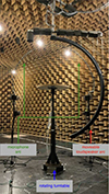 |
Figure 3. The technical setup of the acoustic measurement environment in a hemi-anechoic chamber. |
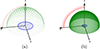 |
Figure 4. Both geometrical setups with the sample in blue. (a) The measurement setup with loudspeaker positions in red and the microphone arc in dark green resulting in a total receiver array in light green after the measurement procedure. (b) The optimal far-field simulation setup with the incidence plane waves in red and the receiver positions in green. |
Instead of a fixed hemispherical microphone array, a microphone arc forms a hemi-circle around the sample. This array consists of 32 calibrated Sennheiser KE4 electret microphones, arranged based on Gaussian sampling [15] of order 31 with a radius of 1 m. Unlike the loudspeaker arc, the microphone arc remains stationary within the room. The relative movement between the sample and the microphone array is achieved by rotating the sample. The Gaussian sampling results in an angular resolution of ΔϑR=5.5° and ΔφR=5.625°.
3.1.2 Measurement procedure
In order to accurately determine the reflected sound pressure from the entire surface of the test sample and the reference surface, both the loudspeaker arc and the turntable are rotated incrementally, allowing the microphones to capture measurements at intervals corresponding to the previously mentioned azimuthal resolution of ΔφR=5.625°. The rotation and the measurement are done via MATLAB [16] and the ITA-Toolbox [17]. Additionally, the turntable is rotated in ΔφS=15° increments to account for different source positions. This entire process takes approximately 8 h. However, if the sample's surface exhibits symmetry, the measurement time can be significantly reduced. For surfaces with symmetry along one axis, the measurement time can be halved. For surfaces with symmetry along two axes, the measurement time can be reduced by a factor of four.
For symmetric 1D surfaces, such as the sine surface, the measurement time can be further reduced because only positions perpendicular to the symmetry axis need to be measured. The sound pressure in the other directions can be projected by multiplying the frequency bins by cosΦ0, where Φ0 is the angle of incidence relative to the x-axis. This method works effectively due to the high frequency resolution. Using this approach, the measurement time can be reduced to approximately 40 min for a 1D symmetric surface and 60 min for a 2D symmetric surface. For validation purposes, however, a complete measurement was performed to confirm the accuracy of the projection method.
The interleaved sweep method is used to measure the impulse responses [18, 19]. The measurements cover a frequency range from 1 kHz to 24 kHz, with a sampling rate of 48 kHz. This frequency range corresponds to Λ/λ=0.2 to 4.5. During the measurement, the temperature and the relative humidity are monitored. The measurement process begins with capturing the total sound pressure, which consists of three components: the direct sound from the loudspeakers; the reflected sound from the sample, including edge diffraction; and reflections from other objects and the rigid floor. The reflected sound pressure from the sample, including the edge diffraction, must be isolated in the next step.
3.1.3 Data processing
To isolate the reflected sound for the reference and the sample measurement, several methods are available. The first method is defined by the ISO standard [2], where the direct sound is removed by subtracting a measurement taken without any sample (free-field) h2(t) from the measurement taken with the sample or reference surface h1(t). Then the signal is deconvolved with the loudspeaker microphone response and afterwards it is windowed using a simple rectangular window.
If conditions remain exactly the same, direct subtraction should eliminate the direct sound entirely, leaving only the reflection. In practice however, the condition are not exactly the same due to small displacements of the hardware, movement of air or small temperature changes in the measurement environment [20]. Therefore, Robinson and Xiang [20] have proposed an optimized subtraction method, based on an optimal gain factor and a sub-sample time shift to minimize residual components of the direct sound in the subtraction. This method is quite time consuming due to the conversion between time and frequency domain, for each step. Müller-Trapet [6] has further optimized this method by solving the whole problem in the frequency domain, which leads to a quicker solving and the following optimization problem (Eq. (4.10), [6]):
 (7)
(7)
Furthermore, Müller-Trapet has compared the optimized subtraction method with a spatial filtering approach in the spherical harmonics domain. The spatial filtering approach is based on the fact that the direct sound is a plane wave and the reflection is a spherical wave. Therefore, the direct sound can be removed by filtering out the plane wave components in the spherical harmonics domain. This method did not lead to better results, therefore is not further discussed here.
In the present study, the sound pressure h2(t) without the sample was windowed to remove the direct sound from later reflections. A Hann window was applied with a maximum time of tmax=100 ms. The reflected sound was then extracted from h1(t) using the optimized method described in equation (7), implemented with SciPy's least squares optimization function [21], as depicted in Figure 5a.
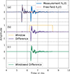 |
Figure 5. Optimized subtraction method and windowing for an incidence angle of ϑS=59.2°, with specular reflection occurring on the reference plate. (a) Specular reflection measurement h1(t) (blue) and free-field measurement h2(t) (red). (b) Resulting subtraction (purple) and Hann window (yellow). (c) Windowed subtraction result (green). |
Then the window for h1(t) was calculated separately for each source-receiver pair based on the travel time of the specular reflection, which defines the shortest reflection path, determined using the image source method and the speed of sound derived from measured temperature and humidity. The window was defined as twindow=(tspec−0.04 ms,tspec+2 ms), leading to a window length of 2.04 ms and resulting in a lower frequency limit of fmin=450 Hz. Figure 5b shows the Hann window used to remove the ground reflection, utilizing the pyfar Python package [22].
The window was selected in a way that the SNR (Signal to Noise Ratio) is maximized. ISO 17497-2 [2] suggests to calculate the SNR based in the windowed area of the subtraction result relative to the noise within the window of h2(t) of the free-field measurement in one-third octave bands. This leads to the following formula:
 (8)
(8)
In our work we have calculated the SNR based on equation (8) and the results are shown in Figure 6 for different incident angles. Although the ISO standard suggests a SNR of at least 40 dB, we could reach a SNR of 20 dB for all incident angles smaller than ϑS=70°. This is due to the fact that for more gazing incidence the direct sound gets closer to the reflected sound and therefore is harder to separate.
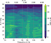 |
Figure 6. Signal-to-Noise Ratio in one-third octave bands from 1 kHz to 20 kHz vs. the incident angle ϑS. |
By measuring all sound pressure data of the sample and of the reference plate, and by utilizing equation (5), we can now calculate the bidirectional scattering coefficient as it was described in the previous section.
3.2 Numerical simulation
The numerical simulation can generally be an alternative for determination of the sound pressure field around the sample according to equation (5).
Furthermore, the numerical modelling can be used to check the influence of the equipment on uncertainties. In this comparison it is possible to validate the measurement results with reference to ideal conditions but with the same geometry.
The simulation software and its postprocessing are published as open source software in Mesh2scattering [23], which is based on Mesh2HRTF [24] and its numerical core NumCalc [25].
The simulation setup is illustrated in Figure 4b. The sound incidence direction in the simulation is the same as that described in Section 3.1.1 for the measurement. The microphone positions represent the upper hemisphere of an equal area grid [26], which provides the best discretization of the sphere while minimizing the number of measurement positions required. The receivers’ distances are set to 80 m, to make sure it is in the far field. This setup results in 11 664 receiver positions leading to an angular resolution of ΔϑR,ΔφR≈1.35°, adhering to the resolution recommendations provided in the relevant standards.
The reference plate is positioned at the center of the simulation, with its upper surface aligned within the x−y plane. The test sample is placed such that the lowest point of its rough surface lies precisely on the x−y plane.
The frequency resolution is set to 1/9th per octave. To minimize the computational effort, two different frequency ranges are used. The first frequency range is from Λ/λ=0.125 to 2, with the samples as depicted in Figures 7a and 7b with 10 repetitions on the surface. For the second frequency range from Λ/λ=2 to 4 a sample with 6 repetitions was used, see Figures 7c and 7d. Appendix A shows the influence of the number of repetitions on the scattering coefficient and concludes a good compromise for lower computational effort and accurate results. All samples are meshed into triangles with an edge length between λ/7 and λ/6 for the shortest acoustic wavelength.
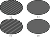 |
Figure 7. Virtual samples used for validation, each with a diameter of d=80 cm, covering two frequency ranges: 0.125≤Λ/λ≤2 (a, b) and 2<Λ/λ≤4 (c, d). (a) Λ=80 mm, n=10. (b) Reference. (c) Λ=133.3 mm, n=6. (d) Reference. |
Since our focus is solely on the reflected sound pressure, the direct sound contribution to the total sound pressure has been deactivated in the computation. By calculating the reflected sound pressure of the sample and of the reference plate, respectively, and by utilizing equation (5), we can now calculate the bidirectional scattering coefficient as it was described in the previous section.
4 Validation
To further validate the experimental procedure and the results on finite-size samples, a sinusoidal test surface of infinite extension was chosen since it already served as reference several times [6–8, 27]. This surface is described by the following equation:
 (9)
(9)
Here, h=20.4 mm is the surface's peak-to-peak height, and Λ=70.8 mm is the structural wavelength. An analytical solution for the scattering coefficient was provided by Embrechts et al. [7]. The analytical solution is compared with numerical simulations and physical measurements. Figure 7 shows the samples for the numerical simulations and Figure 8 depict the samples for the physical measurements.
 |
Figure 8. Physical samples used for validation, each with a diameter of d=80 cm. (a) Λ=70.9 mm, n=11.3. (b) Reference. |
4.1 Results
In the following, scattering coefficients for two specific incident angles and the average over all measured or simulated incidence angles, representing random-incidence are discussed. These bidirectional scattering coefficients are derived by using four methods:
-
the analytical solution for infinite extension,
-
numerical simulations on finite samples based on optimized setup described in Section 3.2,
-
numerical simulations on finite samples based on actual measurement setup from Section 3.1.1,
-
and physical measurements on finite samples.
Thereby it is possible to evaluate the influence of the measurement setup and systematic uncertainties introduced by the measurement process. It is important to note that the measurement setup does not meet the far-field criteria outlined in [2]. The scattering coefficients are then averaged over one-third octave bands.
4.1.1 Larger incident angle
Figures 9a and 9b illustrate the scattered energy at a rather grazing sound incidence of about 62° from the normal. The scattered energy, relative to the total reflected energy, reaches a maximum of 1 at Λ/λ=0.55. This means that at this frequency all energy is scattered, and zero energy is reflected in the specular direction. In Figure 9a, the simulated results show good agreement with the analytical solution. Below Λ/λ=0.5 the scattering coefficient is overestimated, due to the finiteness of the sample and the edge effect, as already known from random-incidence scattering coefficients determination [3, 27]. The scattering coefficient results from the physical measurements are in alignment with the analytical solution, but they are slightly overestimated up to Λ/λ=2. After Λ/λ is 2 they deviate more. Figure 9b shows the one-third octave band representation. Here the measured scattering coefficients are matching well except for Λ/λ=4. Nevertheless, all scattering coefficients in Figures 9a and 9b are within the uncertainty limits of the standard acoustic test methods [27].
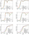 |
Figure 9. Comparison of analytical, simulated, and measured scattering coefficients based on the bidirectional scattering coefficient and in case of random incident of ISO [1] standards (taken from [27]). (a) ϑS=61.74°, no frequency averaging. (b) ϑS=61.74°, one-third octave band averaged. (c) ϑS=31.50°, no frequency averaging. (d) ϑS=31.50°, one-third octave band averaged. (e) Random incidence, no frequency averaging. (f) Random incidence, one-third octave band averaged. |
4.1.2 Smaller incident angle
For the smaller incident angle (steeper incidence) in Figures 9c and 9d, the optimal simulation exhibits a strong agreement with the analytical solution in both representations arise for the notches. This is due to the finite resolution by the given aperture defined by the sample perimeter. While the simulation of the measurement setup generally aligns with the scattering coefficients, discrepancies arise when deep peaks arise. Deviations between the measurement setup and its simulation remain within measurement uncertainties up to Λ/λ=2. However, beyond this threshold, the scattering coefficient is significantly overestimated by the measurement, rendering the results uncertain.
4.1.3 Random incidence
The random-incidence scattering coefficients in Figures 9e and 9f are calculated based on the scattering coefficients from the perpendicular (φS=0°) incident direction using the adapted Paris formula from Embrechts et al. [7], equation (11), except for those taken from literature, which are used as provided.
The simulation with the optimized setup, in Figure 9e shows an strong peak at Λ/λ=1.8, which is not found in the analytical solution, this is due to limited frequency resolution of the simulation. In contrast, the simulation based on the measurement setup, despite having the same frequency resolution, shows better agreement with the analytical solution. Both simulation and measurement demonstrate closer alignment with the analytical solution compared to the ISO measurement in the reverberation room [27]. The simulated measurement setup aligns well with the analytical solution for Λ/λ<2, unlike the case for smaller incident angles (Figs. 9c and 9d). Nevertheless, the results in one-third octave bands are in agreement in a range which is in the same order of magnitude as in the standardized test methods.
5 Bidirectional scattering coefficient
As the measurement setup can deliver a directional scattering pattern, it is now discussed its characteristics and potential application in prediction models. To address this, it is introduced the bidirectional scattering coefficient in the spatial domain.
Figure 10 illustrates a comparison of bidirectional scattering patterns obtained through three different approaches: the analytical solution, optimized setup simulations, and measurements. The analysis is performed for three distinct structural wavelengths divided by the sound wavelength (Λ/λ) under a fixed incident angle of ϑS=29° in red.
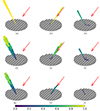 |
Figure 10. Bidirectional scattering coefficients for different incident angles in comparison between analytical solution (infinite sample), and BEM simulation and measurement for the finite sample. The sound incidence is marked by the red arrow. (a) Analytical, Λ/λ=0.5. (b) Analytical, Λ/λ=1.0. (c) Analytical, Λ/λ=2.0. (d) Simulation, Λ/λ=0.5. (e) Simulation, Λ/λ=1.0. (f) Simulation, Λ/λ=2.0. (g) Measurement, Λ/λ=0.5. (h) Measurement, Λ/λ=1.0. (i) Measurement, Λ/λ=2.0. |
The analytical solution of an infinite sinusoidal surface is taken from the work of Embrechts et al. [7], where the bidirectional scattering coefficient for non specular reflections is calculated via two equations. The first equation is describing the direction of the reflected plane waves (see [7], Eq. (2)), while the second one (see [7], Eq. (4)) describes its energy calculation based on the complex reflection factor. Also Rayleigh presented the theory of scattering at periodic surfaces already in 1896 [10]. The distinct angles are hence expected and can well serve as reference.
Comparing the analytical solution with the optimized simulation, the directions of energy reflections are well matching. However, the amount of energy is slightly underestimated in the optimized (BEM) simulation. Especially for lower frequencies, the reflection cone is wider for the simulation. This is due to the finite size of the sample in the simulation and the measurement compared to the infinite surface in the analytical solution. This phenomenon was already observed in previous work [3, 6, 27].
Additionally, this effect is also visible in the width of the reflected cones. Due to the width of the cones, the sum of energy is larger than 1. This is due to the edge effect caused by the finite aperture size [3, 27]. Thus the energy is scattered in a lobe and not into a single narrow direction as in the case of an assumed for infinite structures [3, 13].
The physical measurement shows a similar behavior. This can be also seen in Figures 9c and 9d, where the scattering coefficients are overestimated in the measurement. Future work should focus on quantifying these uncertainties; however, for now, it is assumed that sample size effects in free-field scattering measurements are similar to those observed in [6].
6 Proposal for a data format for bidirectional scattering coefficients
We now have a dataset that includes bidirectional scattering coefficients for different incident directions, scattering directions and frequencies. This dataset can be organized as a three-dimensional data structure:
-
The first dimension represents the incident direction, combining angles ϑS and φS.
-
The second dimension corresponds to the scattering direction, combining angles ϑR and φR.
-
The third dimension represents the frequency.
This structure is illustrated in Figure 11, where the x-axis represents the incident angles, the y-axis represents the reflected angles, and the z-axis represents the frequency. The color indicates the bidirectional scattering coefficient value. According to equation (1), the figure exhibits mirror symmetry along the diagonal, reflecting the reciprocity of the scattering process. As indicated by equation (2), energy conservation is satisfied: the sum over all scattering directions for a given incident direction (i.e., each column in Fig. 11) equals 1, and likewise, the sum over all incident directions for a given scattering direction (i.e., each row) also equals 1. At lower frequencies, the number of available scattering directions decreases, leading to more concentrated energy in the specular direction. Note that the specular energy is located in one element of the cubic dataset for which ϑS=ϑR and φS=φR+πmod2π holds.
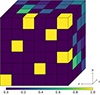 |
Figure 11. Bidirectional scattering coefficient for different incident angles (first dimension, x-axis), the reflected angles (second dimension, y-axis) and the frequency axe (third dimension, z-axis). The colors represent the bidirectional scattering coefficient from 0 to 1 following the colorbar. |
In its current form, the dataset from the measurement includes 1296 incident directions, the same number of scattering directions, and 276 frequency bins. This results in approximately 463.6 million data points, requiring 3.7 GB of memory (assuming 64 bits per floating-point value). The exact size can vary based on the determination method and source resolution. To apply this dataset in sound propagation models, its complexity needs to be reduced by grouping it into specific frequency bands and angular sectors. This reduction is critical for applications. For now, it is not known yet which resolutions in all these dimensions are required for applications in room acoustical and outdoor sound propagation models. This must be investigated in the next steps. The following sections will outline strategies for condensing this dataset into a practical format suitable for sound propagation models, while preserving perceptually significant details.
6.1 Average over octave bands
In geometrical acoustics, the frequency range is typically divided into frequency bands, with absorption and scattering coefficients expressed in these bands. A resolution of one-third octave bands is generally considered sufficient, as it approximately aligns with the Equivalent Rectangular Bandwidths (ERB) in cochlear models.
So far, we have analyzed the surface characteristics relative to the ratio  . Before averaging into the target frequency bands, we must first convert this scale to actual frequencies. This is achieved by incorporating the structural wavelength Λenv and the speed of sound cenv within the virtual environment. The conversion follows the calculation:
 (10)
(10)
After determining the frequencies, the data is averaged across the desired frequency bands using the formula:
 (11)
(11)
Here, sd(f) represents the data at a specific frequency, and the summation is carried out over the range of frequencies from fmin to fmax for the desired band.
Applying this method in our example reduces the number of frequency bins to 10 and the dataset size to approximately 134 MB.
6.2 Angular sectors
In how far the angular resolution can be reduced, must be finally studied in the context of indoor or outdoor propagation simulations and auralizations. For now, we can safely assume that the maximum resolution required is limited by human sound localization capabilities, which are approximately 1 degree in azimuth for frontal incidence in free-field conditions. However, it is reasonable to consider lower resolutions because scattered energy is inherently angularly blurred.
To simplify the angular resolution, we define at first a hemispherical angular grid. Various approaches are possible. An equal-area grid would lead to the most efficient representation, but most sound propagation models can only handle equiangular directivities. Siltanen et al. [12] chose an azimuth and elevation resolution of 30° yielding 36 incident and reflectance directions. Once the angular grid is defined, all previous directions are summed up to the closest new direction. This results in the following formula:
 (12)
(12)
In our example, we chose a resolution of 10° in azimuth and elevation, resulting in 324 incident and reflectance directions. This reduces the size of the dataset to 8.4 MB.
6.3 Data format
How can data be stored and exchanged in the most effective and appropriate way? One candidate is the Spatially Oriented Format for Acoustics (SOFA) standard [28], which defines a data format for spatially oriented acoustic data and is widely utilized for representing source and receiver directivities in both the time and frequency domains. A variety of application programming interfaces (API) are available for common programming languages, facilitating the reading and writing of SOFA data. The SOFA standard also incorporates metadata management, including information on source and receiver positions, measurement metadata, licensing details, and descriptive content.
The format supports the storage of data in either the frequency domain (as transfer functions, TF) or the time domain (as finite impulse responses, FIR). All data is stored in the HDF5 file format, a robust and widely adopted format for scientific data, that supports multidimensional datasets. Although specific conventions for directional scattering data are not yet established, the SOFA standard permits the inclusion of custom fields.
For bidirectional scattering coefficients, it is proposed to extend the GeneralTF specification with the following fields as described in Table 1.
Proposed extra fields for the GeneralTF in the SOFA standard.
The speed of sound and the structural wavelengths are necessary for converting data between Λ/λ (normalized wavelength ratios) and frequencies. Receiver weights are essential for certain surface-based sound propagation models, while source weights are required to compute the random-incidence scattering coefficient. The random-incidence scattering coefficient can be included as it can be directly derived from the bidirectional scattering coefficients.
7 Discussion and conclusion
We presented the technical procedures of a new framework to determine and store bidirectional scattering coefficients for sound propagation models. The determination method can be based on numerical simulation or physical measurements, which were both validated against a well-established reference surface with its analytical solution and previously measured random-incidence scattering coefficients.
The validation of the scattering coefficient and bidirectional scattering coefficient has demonstrated the effectiveness and limitations of the numerical and experimental approaches. The analysis highlights several key observations and limitations. First, the systematic measurement error of the finiteness of the surface and the reflection of the edges, known from the random-incidence scattering coefficient measured in a reverberation chamber [3, 7, 27], can be seen here as well especially for low frequencies. However, in this method, the measurement error is reduced compared to the reverberation room approach, due to the properties of the correlation method. The sd reflection cones, however, are wider and show crosstalk to neighboring cones, so that errors occur in comparison to the analytical reference at lower frequencies. This is due to the aperture effect, i.e., longer wavelengths relative to the finite size of the sample and the angular resolution. At higher frequencies, however, the width of the reflection cones matches the analytical solution.
Another systematic measurement error is made in the measurement setup by not fulfilling the far-field criteria and the required distance between the source and the plate in order to make the assumption of an incident plane wave valid. This can be clearly seen, since the optimized simulation shows good agreement with the analytical solution, while the measurement setup simulation shows a less accurate result. When the results are compared in the usual material and surface data representation in one-third octave bands, the differences are in the order of magnitude of the uncertainty limits of the standard acoustic test methods for random-incidence absorption and scattering [27].
A data format was proposed using the SOFA standard, to store the bidirectional scattering coefficients with all required metadata for exchange.
All steps, from determining the reflected sound pressure distribution to calculating the bidirectional scattering coefficients and averaging them in octave and spatial bands, are well-documented and available as open-access resources.
Due to the limitations of the presented method, the sd must be normalized to ensure that equation (2) is satisfied before being applied in sound propagation models. If an image source model is used separately, the specular reflection component must be removed from sd, and the resulting dataset just contains the bidirectional scattering pattern alone, which well agrees with the separation definition into the energies represented by s and (1−s).
Based on this conceptual approach, detailed investigations shall follow for refining the data representation for various applications in sound propagation modelling. This includes expanding the database with many more documented surface samples and integrating them into the sound propagation models for improved sound scattering modelling. As indicated earlier, the required resolution of the directional bands needs to be determined by perceptual evaluations through auralization of different reference scenes to assess the impact of resolution variations. Then a final recommendation of a required spatial resolution for accurate simulation and auralization can be made.
Acknowledgments
Computations were performed with computing resources granted by RWTH Aachen University under project rwth1245.
Funding
This work was funded by the Deutsche Forschungsgemeinschaft (DFG, German Research Foundation) under the project number 456072683.
Conflicts of interest
The authors declare no conflict of interest.
Data availability statement
The research data associated with this article are available in Zenodo, under the reference https://doi.org/10.5281/zenodo.15673498. The repository contains the measurement results, simulation results, and Python scripts used for the analysis.
Appendix A Number of repetitions
The complexity of the numerical simulation strongly depends on the number of boundary elements (N) for which the BEM has to be solved. For normal BEM this complexity is O(N2) where for the FMM-BEM the complexity is reduced to O(NlogN) [25]. Typically, N≤100 000 elements require less than 16 GB of RAM [25]. However, the number of repetitions increase the diameter of the sample which increase the number of elements. Additionally the increase of Λ/λ increases the number of elements as well, since the size of the elements is between λ/7 and λ/6. Figure A.1 shows the number of elements for different Λ/λ and number of repetitions.
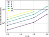 |
Figure A.1. Number of elements of the mesh for different number of structural repetitions. |
Embrechts [13] has shown that the length of a squared sample must be much larger than the acoustic wavelength to yield valid results. This can be reformulated as nΛ/λ≫1, where n is the number of repetitions on the surface. This suggests that at higher frequencies, the number of repetitions can be reduced, leading to lower computational effort in numerical simulations.
Figures A.2 and A.3 show the comparison between analytical and simulated scattering coefficients averaged in one-third octave bands for different number of repetitions on the sample. The results show that the scattering coefficients converge to the analytical solution with increasing number of repetitions, as expected. The lower Λ/λ, the larger the differences between the simulation and the analytical solution. This behavior is also expected since nΛ/λ is smaller for lower Λ/λ. Figure A.2 shows that for Λ/λ>1 the scattering coefficients matches well for all number of repetitions. Figure A.3 shows the same tendencies, but for peaks within the coefficients larger number of repetitions are closer to the analytical reference. Nevertheless, these differences are of the uncertainty limits [27].
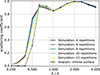 |
Figure A.2. Comparison of analytical and simulated scattering coefficients for varying numbers of repetitions on the sample, averaged over one-third octave bands at an incident angle of ϑS=61.74°. |
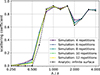 |
Figure A.3. Comparison of analytical and simulated scattering coefficients for varying numbers of repetitions on the sample, averaged over one-third octave bands at an incident angle of ϑS=31.5°. |
Therefore for simulations of range 0.125≤Λ/λ≤2, n=10 repetitions were used and for simulations of range 2≤Λ/λ≤4, n=6 repetitions were chosen. This leads to a large reduction of the computational effort for the numerical simulations and holds the number of boundary elements on the mesh below 100 000.
References
- ISO 17497-1:2004: Sound-scattering properties of surfaces. Part 1: measurement of the random-incidence scattering coefficient in a reverberation room. International Organization for Standards, Geneva, Switzerland, 2004 [Google Scholar]
- ISO 17497-2:2012: Sound-scattering properties of surfaces. Part 2: measurement of the directional diffusion coefficient in a free field. International Organization for Standards, Geneva, Switzerland, 2012 [Google Scholar]
- T. Cox, P. d’Antonio: Acoustic Absorbers and Diffusers: Theory, Design and Application, 3 edition. CRC Press, 2016 [Google Scholar]
- E. Mommertz: Determination of scattering coefficients from the reflection directivity of architectural surfaces. Applied Acoustics 60, 2 (2000) 201–203 [Google Scholar]
- H. Kuttruff: Room Acoustics, 6th edition. CRC Press/Taylor & Francis Group, Boca Raton, 2017 [Google Scholar]
- M. Müller-Trapet: Measurement of surface reflection properties: concepts and uncertainties. Dissertation, Logos-Verl., Berlin, 2015 [Google Scholar]
- J. Embrechts, L.D. Geetere, G. Vermeir, M. Vorländer, T. Sakuma: Calculation of the random-incidence scattering coefficients of a sine-shaped surface. Acta Acustica United with Acustica 92 (2006) 593–603 [Google Scholar]
- Y. Kosaka, T. Sakuma: Numerical examination on scattering coefficients of architectural surfaces using the boundary element method. Acoustical Science and Technology 26, 2 (2005) 136–144 [Google Scholar]
- J.-J. Embrechts, A. Billon: Theoretical determination of the random-incidence scattering coefficients of infinite rigid surfaces with a periodic rectangular roughness profile. Acta Acustica United with Acustica 97, 4 (2011) 607–617 [Google Scholar]
- J.W.S.B. Rayleigh: The Theory of Sound. Vol. 11 of New York Dover Publications, 2nd edition. Macmillan, 1896 [Google Scholar]
- F.E. Nicodemus, J. Richmond, J. Hsia, I. Ginsberg, T. Limperis: Geometrical Considerations and Nomenclature for Reflectance. Vol. 160. US Department of Commerce, National Bureau of Standards Washington, DC, USA, 1977. http://graphics.stanford.edu/courses/cs448-05-winter/papers/nicodemus-brdf-nist.pdf [Google Scholar]
- S. Siltanen, T. Lokki, S. Kiminki, L. Savioja: The room acoustic rendering equation. The Journal of the Acoustical Society of America 122, 3 (2007) 1624–1635 [Google Scholar]
- J.J. Embrechts, D. Archambeau, G.B. Stan: Determination of the scattering coefficient of random rough diffusing surfaces for room acoustics applications. Acta Acustica United with Acustica 87, 4 (2001) 482–494 [Google Scholar]
- J.-G. Richter, J. Fels: On the influence of continuous subject rotation during high-resolution head-related transfer function measurements. IEEE/ACM Transactions on Audio, Speech, and Language Processing 27, 4 (2019) 730–741 [CrossRef] [Google Scholar]
- B. Rafaely: Fundamentals of Spherical Array Processing. Vol. 16. Springer, 2018 [Google Scholar]
- The-MathWorks-Inc.: MATLAB version: 9.13.0 (R2022b), 2022. https://www.mathworks.com [Google Scholar]
- M. Berzborn, R. Bomhardt, J. Klein, J.-G. Richter, M. Vorländer: The ITA-toolbox: an open source MATLAB toolbox for acoustic measurements and signal processing, in: Fortschritte der Akustik – DAGA 2017. 43th Annual German Congress on Acoustics, Kiel (Germany), 6 Mar 2017–9 Mar 2017, Mar. 2017. http://publications.rwth-aachen.de/record/687308 [Google Scholar]
- P. Massarani: Transfer-function measurement with sweeps. Journal of the Audio Engineering Society 49, 6 (2001) 443–471 [Google Scholar]
- P. Dietrich, B. Masiero, M. Vorländer: On the optimization of the multiple exponential sweep method. Journal of the Audio Engineering Society 61, 3 (2013) 113–124 [Google Scholar]
- P. Robinson, N. Xiang: On the subtraction method for in-situ reflection and diffusion coefficient measurements. The Journal of the Acoustical Society of America 127, 3 (2010) EL99–EL104 [Google Scholar]
- P. Virtanen, R. Gommers, T.E. Oliphant, M. Haberland, T. Reddy, D. Cournapeau, E. Burovski, P. Peterson, W. Weckesser, J. Bright, S.J. van der Walt, M. Brett, J. Wilson, K.J. Millman, N. Mayorov, A.R.J. Nelson, E. Jones, R. Kern, E. Larson, C.J. Carey, İ. Polat, Y. Feng, E.W. Moore, J. VanderPlas, D. Laxalde, J. Perktold, R. Cimrman, I. Henriksen, E.A. Quintero, C.R. Harris, A.M. Archibald, A.H. Ribeiro, F. Pedregosa, P. van Mulbregt, SciPy 1.0 Contributors: SciPy 1.0: fundamental algorithms for scientific computing in python. Nature Methods 17 (2020) 261–272 [CrossRef] [Google Scholar]
- pyfar-developers: pyfar version: 0.6.8 (python 3.10), 2024. https://www.pyfar.org [Google Scholar]
- A. Heimes: mesh2scattering version: 1.0.0 (python 3.10), 2025. https://github.com/ahms5/Mesh2scattering [Google Scholar]
- F. Brinkmann, W. Kreuzer, J. Thomsen, S. Dombrovskis, K. Pollack, S. Weinzierl, P. Majdak: Recent advances in an open software for numerical HRTF calculation. Journal of the Audio Engineering Society 71, 7/8 (2023) 502–514 [Google Scholar]
- W. Kreuzer, K. Pollack, F. Brinkmann, P. Majdak: NumCalc: an open-source BEM code for solving acoustic scattering problems. Engineering Analysis with Boundary Elements 161 (2024) 157–178 [Google Scholar]
- P. Leopardi: A partition of the unit sphere into regions of equal area and small diameter. Electronic Transactions on Numerical Analysis 25, 12 (2006) 309–327 [Google Scholar]
- M. Vorländer, J.-J. Embrechts, L. De Geetere, G. Vermeir, M.H. de Avelar Gomes: Case studies in measurement of random incidence scattering coefficients. Acta Acustica united with Acustica 90, 5 (2004) 858–867 [Google Scholar]
- AES Standards Comittee: AES69-2022: AES standard for file exchange – Spatial acoustic data file format, 2022. https://www.aes.org/publications/standards/search.cfm?docID=99 [Google Scholar]
Cite this article as: Heimes A. & Vorländer M. 2025. Bidirectional surface scattering coefficients. Acta Acustica, 9, 41. https://doi.org/10.1051/aacus/2025026.
All Tables
All Figures
|
Figure 1. Comparison of Lambertian and real energetic sound scattering pattern. A plane wave with incidence in (green) hits a rough periodic surface (black). The reflection pattern of a sinusoidal surface (red) at Λ/λ=2 is determined after Embrechts analytical solution [7] including its direction and energy. The Lambertian model (blue) is discretized in equal angular steps of 15°. The length of the arrows represent their energies. Both reflection patterns result in a random-incident scattering coefficient of 1 as they are normalized in energy. |
| In the text | |
|
Figure 2. Definition of the coordinate system with the surface under investigation in blue. The incident sound direction is marked in red, where the scattered direction is marked in green. |
| In the text | |
|
Figure 3. The technical setup of the acoustic measurement environment in a hemi-anechoic chamber. |
| In the text | |
|
Figure 4. Both geometrical setups with the sample in blue. (a) The measurement setup with loudspeaker positions in red and the microphone arc in dark green resulting in a total receiver array in light green after the measurement procedure. (b) The optimal far-field simulation setup with the incidence plane waves in red and the receiver positions in green. |
| In the text | |
|
Figure 5. Optimized subtraction method and windowing for an incidence angle of ϑS=59.2°, with specular reflection occurring on the reference plate. (a) Specular reflection measurement h1(t) (blue) and free-field measurement h2(t) (red). (b) Resulting subtraction (purple) and Hann window (yellow). (c) Windowed subtraction result (green). |
| In the text | |
|
Figure 6. Signal-to-Noise Ratio in one-third octave bands from 1 kHz to 20 kHz vs. the incident angle ϑS. |
| In the text | |
|
Figure 7. Virtual samples used for validation, each with a diameter of d=80 cm, covering two frequency ranges: 0.125≤Λ/λ≤2 (a, b) and 2<Λ/λ≤4 (c, d). (a) Λ=80 mm, n=10. (b) Reference. (c) Λ=133.3 mm, n=6. (d) Reference. |
| In the text | |
|
Figure 8. Physical samples used for validation, each with a diameter of d=80 cm. (a) Λ=70.9 mm, n=11.3. (b) Reference. |
| In the text | |
|
Figure 9. Comparison of analytical, simulated, and measured scattering coefficients based on the bidirectional scattering coefficient and in case of random incident of ISO [1] standards (taken from [27]). (a) ϑS=61.74°, no frequency averaging. (b) ϑS=61.74°, one-third octave band averaged. (c) ϑS=31.50°, no frequency averaging. (d) ϑS=31.50°, one-third octave band averaged. (e) Random incidence, no frequency averaging. (f) Random incidence, one-third octave band averaged. |
| In the text | |
|
Figure 10. Bidirectional scattering coefficients for different incident angles in comparison between analytical solution (infinite sample), and BEM simulation and measurement for the finite sample. The sound incidence is marked by the red arrow. (a) Analytical, Λ/λ=0.5. (b) Analytical, Λ/λ=1.0. (c) Analytical, Λ/λ=2.0. (d) Simulation, Λ/λ=0.5. (e) Simulation, Λ/λ=1.0. (f) Simulation, Λ/λ=2.0. (g) Measurement, Λ/λ=0.5. (h) Measurement, Λ/λ=1.0. (i) Measurement, Λ/λ=2.0. |
| In the text | |
|
Figure 11. Bidirectional scattering coefficient for different incident angles (first dimension, x-axis), the reflected angles (second dimension, y-axis) and the frequency axe (third dimension, z-axis). The colors represent the bidirectional scattering coefficient from 0 to 1 following the colorbar. |
| In the text | |
|
Figure A.1. Number of elements of the mesh for different number of structural repetitions. |
| In the text | |
|
Figure A.2. Comparison of analytical and simulated scattering coefficients for varying numbers of repetitions on the sample, averaged over one-third octave bands at an incident angle of ϑS=61.74°. |
| In the text | |
|
Figure A.3. Comparison of analytical and simulated scattering coefficients for varying numbers of repetitions on the sample, averaged over one-third octave bands at an incident angle of ϑS=31.5°. |
| In the text | |
Current usage metrics show cumulative count of Article Views (full-text article views including HTML views, PDF and ePub downloads, according to the available data) and Abstracts Views on Vision4Press platform.
Data correspond to usage on the plateform after 2015. The current usage metrics is available 48-96 hours after online publication and is updated daily on week days.
Initial download of the metrics may take a while.