| Issue |
Acta Acust.
Volume 9, 2025
|
|
|---|---|---|
| Article Number | 40 | |
| Number of page(s) | 19 | |
| Section | Active Control | |
| DOI | https://doi.org/10.1051/aacus/2025020 | |
| Published online | 16 July 2025 | |
Review Article
Electro-acoustic control of radiation impedance for brass instrument timbre shaping: design of a vocalizing mute
1
S3AM-STMS-Sorbonne Université-Ircam 1, Place Igor Stravinsky 75004 Paris France
2
S3AM-STMS-CNRS-Ircam 1, Place Igor Stravinsky 75004 Paris France
3
Mines Paris – PSL, Center of Robotics 60 bd Saint-Michel 75006 Paris France
* Corresponding author: This email address is being protected from spambots. You need JavaScript enabled to view it.
Received:
20
August
2024
Accepted:
10
May
2025
Abstract
The application of active control to musical instruments brings many benefits to composers and performers, by expanding their sound possibilities. This paper addresses the active control of a brass instrument to design a vocalizing mute. To this end, a sensor (pressure transducer) and an actuator (loudspeaker) with a feedback loop are placed at the bell extremity. A single-input single-output controller is designed to simulate the insertion of a flow-to-flow vocal filter, upstream of the natural radiation impedance load. The vocal transfer function with its target resonances is basically derived using the transfer matrix method for a vocal tract composed of concatenated acoustic cylinders. The loudspeaker model is based on the Thiele and Small description. Numerical experiments are presented on the controller, for a simplified trombone model that admits a Kelly-Lochbaum structure (mouthpiece, bore, bell and radiation are cascaded using the transfer matrix method). Finally, the sensitivity of the control to air temperature, bell opening angle and loudspeakers parameters is studied.
Key words: Active control / Augmented brass instrument / Formants
© The Author(s), Published by EDP Sciences, 2025
 This is an Open Access article distributed under the terms of the Creative Commons Attribution License (https://creativecommons.org/licenses/by/4.0), which permits unrestricted use, distribution, and reproduction in any medium, provided the original work is properly cited.
1 Introduction
Active control serves as a versatile technique for modifying the vibrations of a system through the use of transducers. It was first used in noise reduction (cf. Lueg patent to suppress pure tones in pipes [1], Fogel for noise reduction in aircraft cockpits [2]). It has also been used for several years on musical instruments enabling the creation of so-called augmented instruments. The first piano with an active control system was patented in 1893 [3] by Eisenmann, on which a controller extended the string vibration using electromagnets. Feedback controllers based on the same principle have been developed more recently for electric guitar strings [4, 5]. In the family of percussion instruments, active modal control has also been developed to control the vibration modes of a xylophone bar [6]. Concerning wind instruments, active control has been used to modify the input impedance of a clarinet [7] and to study nonlinear couplings with its resonator [8]. This paper is part of the general study of active control applied to brass instruments.
Playing vowels with instruments can produce a spectacular effect, for example with hand movements in front of a trombone bell in the manner of a Kempelen machine [9], or with dedicated mutes, as in the case of S. Turre or P. Eötvös in the piece Snatches of Conversation, who uses an association of Pixie and Plunger mutes. Also, using active control to modify the sound of brass instruments has a number of advantages. Thus, during performance, a brass player naturally controls his instrument through auditory feedback (radiated sound) and haptic feedback (felt through the vibration of his lips), which are correlated. By using active control, which allows the instrument to produce new sounds by modifying its own vibration (that of its air column), this correlation is preserved. This is in contrast to usual sound effects, which act on recorded sound and then play it back through loudspeakers. For these two reasons, this study aims to design a vocalizing mute using active control. To do that, we propose to modify the radiation impedance of a trombone, in order to simulate the presence of a human vocal tract downstream of its resonator. The choice of the geometry of the simulated vocal tract will make it possible to produce new trombone sounds by applying a spectral envelope similar to that of human vowel sounds. This article follows on from [10], which presents the first theoretical results. The simulations are improved using a Kelly-Lochbaum structure, and an analysis of the controller sensitivity is added.
The paper is organised as follows. Section 2 presents a global block diagram of the instrument (from the performer's mouth cavity to the acoustic radiation), introduces the control block inserted to achieve the objective, and sets out the working hypotheses on which the control law will be designed. Section 3 details basic passive acoustic modellings of radiation impedance and of the vocal tract to be virtualised. They are presented in the spectral domain (Laplace and Z). Section 4 is devoted to the design of the acoustic control law that achieves the target behaviour. It also examines its robustness through a sensitivity analysis. Then, Section 5 focuses on the sensors and actuators. It introduces their modelling with parameters and then derives the electro-acoustic feedback law to be implemented between these transducers. Finally, Section 6 presents numerical experiments and discusses the impact of the active control method developed in this article on the waveform and spectrum of the radiated sound.
2 Problem statement
This section sets out the work basis chosen in this paper to modify a trombone and make it radiate vowels.
It describes the played instrument in the form of a block diagram (Sect. 2.1) used to formulate the objective (Sect. 2.2) and the working hypotheses (Sect. 2.3). It then presents the control structure (Sect. 2.4), on the basis of which the control law will be designed (Sect. 2.5).
2.1 Structure of a played trombone and acoustic elements
Addressing the control of the trombone under realistic playing conditions requires consideration of several working constraints, such as:
(C1): complex aero-acoustic coupling with lips [11, 12],
(C2): complex modelling of visco-thermal losses inside the pipe [13–17],
(C3): both longitudinal and transverse modes above approximately 1250 Hz (see [18, Fig. 4]), which overlap the frequency range of the targeted application (the first four vowel resonances typically lying between 250 Hz and 4 kHz),
(C4): time-varying length due to slide movements when playing,
(C5): nonlinear propagation at high playing levels (see [19, 20] for modelling and [21] for sound synthesis).
This is witnessed by many studies and a large literature; see, e.g., [22] and the references therein.To address these constraints and prepare an effective control strategy, the instrument is first decomposed into several blocks, as shown in Figure 1:
Block A: represents the complex dynamical system composed of the performer excitation coupled to the acoustic bore until the acoustic state (pressure, airflow) at the bell extremity,
Block B: represents the radiation load experienced by this state at the bell extremity,
Block C: represents how this state propagates into the room, including directivity effects.
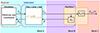 |
Figure 1. Block diagram of a played trombone in its environment. First, the pipe is described by a quadripole. The two inputs are the mouthpiece volumetric flow rate, denoted Uin and the pressure at the bell, denoted P. The two outputs are the flow rate at the bell, Utb and the mouthpiece pressure Pin. Second, the radiation is represented by a linear impedance load ZR (equal to P/Utb in the Laplace domain). And the transfer impedance TR(r) between Utb and the pressure Pout(r) at a point r. Note that in all the paper, flow rates are algebraic quantities counted positively in the direction of eℓ (e.g., Uin=Uineℓ). |
Figure 1 also introduces notations and conventions used within this paper.
2.2 Objective
Our objective is to develop a control method that operates effectively and independently of constraints (C1)–(C5) to make the trombone radiates vowels.
Strategy. We choose to work only on block B, by introducing a controller with a feedback loop, as proposed in Figure 2: the natural bell flow Utb is augmented by an additional component Uac for reshaping the radiation load, using a control, to meet a target. In the block diagram, this insertion is acoustically implemented at the isobar located at the bell extremity (see hypotheses below). It operates as a conservative junction with three ports, all of which share the same pressure and effectively balances all incoming flow rates. Following the orientation convention for flow rates, this balance equation reads UR=Uac+Utb.
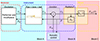 |
Figure 2. Block diagram of the musical instrument equipped with active control. Note that with no control (Uac=0), we recover the Figure 1 (UR=Utb). |
Target. In this paper, active control is used to simulate the presence of a vocal tract downstream of the trombone resonator, an organ that, in humans, extends from the glottis to the bucconasal cavity. Here, the nasal cavity is assumed to be closed by the soft palate, which allows only nonnasal vowels to be produced. The vocal tract is therefore considered an unbranched tube with a single input, the incoming flow rate on the glottis side, and a single output, the outgoing flow rate on the lips side. As the simulated vocal tract is placed at the output of the trombone resonator, according to the notations shown in Figure 2, these two flow rates are equal to Utb and UR respectively. The goal is to modify the radiated airflow as
 (1)
(1)
where HVT represents the vocal tract transfer function in the Laplace domain, that relates the airflow at the glottis to the airflow at the lips for a given vowel.
2.3 Hypotheses
The following assumptions are made, focusing exclusively on Block B in alignment with the strategy and objective:
(H1): Radiation load: approximated by a linear time-invariant passive impedance on a spherical cap (model chosen in Sect. 3.1);
(H2): Vocal tract (target): modeled by a linear time-invariant transfer function that relates the airflow at the glottis to the airflow at the lips (model chosen in Sect. 3.2);
(H3): Controller: linear time invariant feedback-loop between transducers (sensors and actuators) also assumed to be linear (design in Sects. 2.4 and 5.2). In this theoretical study, transducers are supposed to be co-located and distribute a homogeneous acoustic control over the spherical cap.
2.4 Control structure
The overall structure of the controller is shown in Figure 3. As explained in the objective, in Section 2.2, it takes the bell pressure as its only input. According to hypothesis of co-located control (H3), the loudspeaker generates a contribution Uac at the bell, which is added to the outgoing flow rate of the trombone Utb, so that the total flow rate is equal to Utb+Uac on the spherical isobar where the microphone is placed. As a consequence, this spherical isobar can be seen as a junction linking the two systems {Trombone Resonator} and {Controller}, which are fed by the same input, and whose outputs add up to each other.
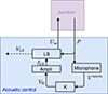 |
Figure 3. Block diagram in the Laplace domain of the overall control structure. It is composed of a microphone (transfer function between acoustic pressure P and voltage Vmicro), a controller (cascaded transfer functions K and Ampli between voltage Vmicro) and current ILS and a loudspeaker LS (quadripole with two inputs – pressure P and current ILS – and two outputs – voltage VLS and flow rate Uac). |
For sake of simplicity, the microphone is described as a linear pressure-to-voltage converter with unit gain. The loudspeaker behaves like an electrical current to acoustical flow converter. Thus, between these two transducers, the controller designed to impose the desired vocal tract transfer function between Utb and UR, must convert a voltage into a current. For later experimental implementation, the controller transfer function is separated into two cascaded parts:
-
the one, called Ampli in Figure 3, converts a voltage into a current with unit gain. An electronic solution of design has been proposed by Mc Pherson, based on a feedback loop circuit including an operational amplifier [23].
-
the other, called K, which must therefore supply an electrical voltage, can thus be implemented in a conventional digital signal processor. Its expression is derived in Section 5.
2.5 Summary
In summary, this paper proposes the design of an active control system, localised at the bell, that operates as a targetable mute. Note that, as standard mutes do, such control impacts the entire instrument and the acoustic boundary conditions experienced by the musician's lips (the input impedance in the linear time-invariant case of a static bore at low amplitude levels). In this context, the active control is not merely an electronic vocoder effect played back through external loudspeakers.
3 Radiation impedance ZR and vocal tract HVT modeling
This section presents models of the components required for calculating the acoustic control law (transfer function K). These models refer to the components of Block B presented in Figure 2 (see Sect. 2.2): the radiation impedance ZR (in Sect. 3.1) and the vocal tract transfer function HVT (in Sect. 3.2). A particular attention is paid to the choice of its modelling, which results from a compromise between realism (consideration of non-planar wavefronts) and simplicity.
3.1 Radiation
Several acoustic radiation models are available (see e.g., [24, 25] for a review of classical models) for the 1D modelling of musical instruments. A first interest of the work proposed in [26] is to account for the effect of isobar curvature at the bell outlet, by assuming that the bell radiates similarly to a pulsating spherical cap (see Fig. 4). A second interest is to approximate the impedance formula (decomposed over spherical harmonics) with optimised simpler differential models. The model chosen here is the second-order high-pass filter described below, which exhibits better results than classical 1D planar models (see [27, 28]).
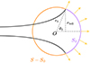 |
Figure 4. Radiation model of the bell of a wind instrument. The purple spherical cap S0 is the uniformly animated part and the orange cap S−S0 is motionless (see details in [26]). |
This radiation impedance  is modelled in the Laplace domain by
 (2a)
(2a)
 (2b)
(2b)
where (see Tab. 1) ρ0 and c0 are the air density and the speed of sound, r0 is the sphere radius, θ0 is the cap half-angle ( ), and where optimal parameters α, ξ and νc are given by the following functions, defined for all
 ![Mathematical equation: $ \theta _0\in [0,\frac {\pi }{2}] $](/articles/aacus/full_html/2025/01/aacus240106/aacus240106-eq6.gif) ,
,  ,
,  and
and  .
.
The Laplace region of convergence of ZR includes  (denoting
  ) and it is proved to define a causal, stable, passive system [26, 28] which therefore meets the expectations formulated in (H1), Section 2.3. Figure 5 shows the values of module and phase of
  for several values of θ0.
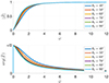 |
Figure 5. Bode diagram of adimensioned radiation impedance |

Note that the cutoff frequency (for which  ) is given by
 ![Mathematical equation: $ f_c = \frac {c_0}{r_0}\nu _c [[1 + \beta ^2]^\frac {1}{2} - \beta ]^\frac {1}{2} $](/articles/aacus/full_html/2025/01/aacus240106/aacus240106-eq18.gif) with β=1+α2−2ξ2. For typical values measured on a real trombone bell, θ0=72.4° and r0=8.39 cm, fc is equal to 893 Hz.
with β=1+α2−2ξ2. For typical values measured on a real trombone bell, θ0=72.4° and r0=8.39 cm, fc is equal to 893 Hz.
3.2 Vocal tract
To design the vocal effect subsequently applied by active control to the radiated impedance of the trombone, we consider a static vocal tract (producing one vowel, see (H2)). Then, we need a model of its flow-to-flow filter (see (1)), the resonances of which are related to formants and characterise the vowel. This linear time-invariant causal filter is derived by considering NVT cascaded straight pipes of equal length and of cross-section area an (see Fig. 6), radiating in a semi-infinite end pipe of cross-section area aext. As proposed by Mathur et al. [29], their length, equal to 3.968 mm, is slightly greater than the distance covered in half a sampling period. This allows the vocal tract to vary in length and leads to a more realistic synthesis. This filter admits a standard Kelly-Lochbaum structure [30, 31] with relevant computational details provided in Appendix D to ensure self-consistency (see Fig. D.1 and Eqs. (D.1), (D.2)).
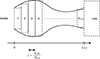 |
Figure 6. Modelling the vocal tract. |
The vocal tract transfer function HVT=Uout/Uin is derived from the transfer matrix TVT of the cascaded pipes loaded by a radiation impedance  , so that
![Mathematical equation: $$ {\left [\begin {array}{c} P_{\mathrm {in}}\\ U_{\mathrm {in}} \end {array}\right ]} = \mathop {\underbrace {T_{\mathrm {VT}} {\left [\begin {array}{c} Z_{\mathrm {R}}^{\mathrm {VT}}\\ 1 \end {array}\right ]}}}\limits _{{\left [\begin {array}{c} * \\ H_{\mathrm {VT}}^{-1} \end {array}\right ]}} U_{\mathrm {out}}. $$](/articles/aacus/full_html/2025/01/aacus240106/aacus240106-eq20.gif) (3)
(3)
Figure 7 shows the Bode diagram of HVT computed for the vowel [a] described by the area profile in Figure 8 and choosing1 aext=38.2 cm2.
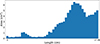 |
Figure 7. Bode diagram of the transfer function HVT(s=2iπf) of a vocal tract for the vowel profile [a] (see Fig. 8), loaded by |
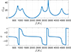 |
Figure 8. Area profile of the vocal tract for vowel [a] extracted from [31, Table 3] (NVT=44 cascaded pipes, total length LVT=17.46 cm, so that LVT/NVT=3.968 mm). |
4 Target acoustic control
This section introduces the control law designed within the acoustic domain to achieve the desired behaviour. This law relies solely on the radiation impedance ZR and the transfer function HVT of the target vowel2. Subsequently, the robustness of vowel rendering is evaluated. Initially, a basic test examines deviations due to an angle error θ0 in the radiation impedance model. Following this, a sensitivity analysis with respect to θ0 and temperature T is presented.
4.1 Control model
As mentioned in Section 1, the target application is to produce a vocalised version of the radiated sound. This amounts to applying resonances (through HVT) to the radiated pressure (originally generated by the trombone flow rate Utb). To this end, the principle consists of adding a controlled acoustic flow rate (Uac) to that of the trombone (Utb) at the bell extremity in order to form a modified version of the flow rate (UR=Utb+Uac) experienced by the natural acoustic radiation. This is implemented by adding a flow source, assumed to be ideal in the low frequency range (H1), so that it defines an ideal conservative junction with three ports, that balances flows and equalises pressures (see Fig. 2), that is,
 (4a)
(4a)
 (4b)
(4b)
Then, the control is designed such that the flow experienced by the radiation (UR) becomes a vocalised version of the trombone flow (HVTUtb) rather than the trombone flow itself (Utb), that is (see Fig. 9)
 (5)
(5)
Note that, from the trombone viewpoint, this amounts to loading its bell extremity by the modified radiation impedance HVTZR, denoted  below.
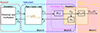 |
Figure 9. Block diagram of the target radiation impedance in the Laplace domain. Here, the vocal tract HVT is placed between the pipe and the radiation such that the new radiation flow rate UR is now equal to UR=HVTUtb. |
Then, modelling the acoustic control by its admittance Yac=Uac/Pac, it follows from (4a) that, at the acoustic junction,
 (6a)
(6a)
The expected target (UR=HVTUtb) is achieved if  , so that (6a) becomes
 (6b)
(6b)
Finally, from (4b), the target acoustic control admittance is
 (7a)
(7a)
leading to the equivalent formula for the vocal tract filter
 (7b)
(7b)
4.2 Qualitative robustness test
Denote  the target vocal filter. Denote
  the exact (but unknown) radiation impedance and
  the (possibly) erroneous model.
Following (7a), the acoustic control we compute for  and
and  leads to
  . Using this control
  , the vocal filter produced in reality by the exact radiation
  is, following (7b)
  , that is
 (8)
(8)
Following this equation, the relative errors
 (9a)
(9a)
committed respectively on the vocal filter and on the radiation impedance, are related by
 (9b)
(9b)
A robustness test is presented for  given in Figure 7 where
  , with parameter
  (see (2a), (2b) and Tab. 1), is erroneously replaced by
  , with the same parameters except a deviation of +5% on the angle
  (see Fig. 10).
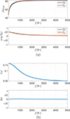 |
Figure 10. Bode diagrams: (a) radiation impedances |


The vocal tract filter  resulting from (8) is compared to
  in Figure 11: the peaks are modified (see Tab. 2) but are still qualitatively representative of a vowel [a]. In the following section, we complete this test by a sensitivity analysis.
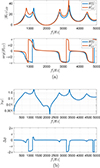 |
Figure 11. Bode diagrams: (a) vocal tract filters H† (exact, in red) and Herr (erroneous, in blue); (b) error characterisation. (a) vocal tract filters: (top) modulus in dB; (bottom) phase in radians. (b) error: (top) relative error modulus |ϵH| (log scale); (bottom) phase deviation Δϕ=ϕerr−ϕ†. |
Comparison of the frequencies Fk and amplitudes Ak of the first five peaks of H† and Herr.
4.3 Sensitivity analysis
In this section, we analyse the sensitivity of HVT to the parameters a=(T,θ0), assuming that:
-
a target control
 is pre-computed from (7a) with fixed parameters T†=300 K,
  ,
, -
the radiation impedance is subject to small variations in its parameters a around
 , and is renoted ZR(s;a).
In this case, the dependency of the vocal tract filter to parameters a reads, from (7b),
 (10a)
(10a)
Then, the first order expansion of HVT(s;a†+δa) with respect to δa1=δT and δa2=δθ0 leads to
 (10b)
(10b)
introducing  and the sensitivity functions for a1=T and a2=θ0 as
 (10c)
(10c)
From (10a), it follows that
 (11a)
(11a)
where  is derived from the chain rule applied to (2a), (2b) in which ρ0, c0, S0, ω0 are the a-dependent functions
 (12a)
(12a)
 (12b)
(12b)
 (12c)
(12c)
 (12d)
(12d)
and α(θ0), ξ(θ0) and νc(θ0) are detailed in Section 3.1.
The physical values of parameters are given in Table 3.

Note that detailing the expression of the sensitivity functions of the characteristic impedance
 (13)
(13)
involved in (2a) yields
 (14a)
(14a)
 (14b)
(14b)
Figure 12 reveals that variations in θ0 and T have a significant impact on the position and amplitude of vocal tract resonances, potentially modifying the radiated vowel. In particular, overestimation of θ0 tends to separate resonances 1 & 2 on the one hand, and 3 & 4 on the other, and to reduce the 5th resonance frequency. Underestimation of θ0 has the opposite effect, fusing resonances 1 & 2 when θ0=80 °. Estimation errors on T cause resonance frequencies to move in the same direction as estimation errors on θ0, but to a lesser extent, at usual temperatures. Indeed, previous measurements carried out with real players [32] show that the temperature in the bore generally rises while playing from room temperature to around 37.7 °C, the temperature of the human body, inducing typical variations of the order of 10 °C. Consequently, an incorrect temperature estimate should have a negligible effect on the vocal tract resonances applied to the radiated sound.
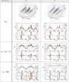 |
Figure 12. Bode diagram (modulus and phase) of the vocal tract filter HVT. The variation in the value of the ai parameters is studied in order to observe the changes in the transfer function. The errors |


5 Electro-acoustic implementation
The active control solution implemented uses a loudspeaker at the end of the bell as an actuator. Section 5.1 presents a brief reminder on its standard linear electro-acoustic modelling with Thiele and Small parameters [33, 34]. In this paper the loudspeaker is driven by a current source assumed to be ideal on the frequency range of interest. Note that the natural causal electric input of a loudspeaker is the voltage (and not the current). This means that the current source requires the use of a dedicated feedback-loop circuit involving an operational amplifier (see e.g., [23]). The output current (see Fig. 3) is governed by ILS=K Vmicro where Vmicro=KmicP denotes the voltage delivered by a pressure microphone of ideal gain Kmic. The pressure-to-current gain is then described by ILS=KtotP with Ktot=K·Kmic.
The transfer function Ktot is the electronic control to be determined in Section 5.2, in order to realise the acoustic target Yac given the loudspeaker model.
5.1 Loudspeaker modelling
A basic linear description of the loudspeaker (LS) is modelled by the following electrical and mechanical equations, cf. [33, 34]:
 (15a)
(15a)
 (15b)
(15b)
where Mms is the mass of the driver diaphragm and voice-coil assembly, Rms and Cms the mechanical resistance and compliance (suspension, spider, acoustic chamber) and Sd the equivalent surface area of the cone. Bl is the coefficient of the magnetic force induced by the current passing through the voice-coil of length l. This model admits the following input (u) – state (x) – output (y) representation:
 (16a)
(16a)
![Mathematical equation: $$ \mathrm {with\ } u = {\left [\begin {array}{c} v_{\mathrm {LS}}\\ P \end {array}\right ]}, \ x = {\left [\begin {array}{c} i_{\mathrm {LS}}\\ z\\ {\dot {z}} \end {array}\right ]}, \ y = {\left [\begin {array}{c} i_{\mathrm {LS}}\\ U_{\mathrm {LS}} \end {array}\right ]}, $$](/articles/aacus/full_html/2025/01/aacus240106/aacus240106-eq83.gif) (16b)
(16b)
![Mathematical equation: $$ A = {\left [\begin {array}{ccc} - \frac {1}{\tau _{\mathrm {e}}} &\quad 0 &\quad - Bl\beta _{\mathrm {e}} \\ 0 &\quad 0 &\quad 1 \\ Bl\beta _{\mathrm {m}} &\quad -\omega _{\mathrm {m}}^2 &\quad - \frac {1}{\tau _{\mathrm {m}}} \end {array}\right ]}\!, \ B = {\left [\begin {array}{cc} \beta _{\mathrm {e}} &\quad 0 \\ 0&\quad 0 \\ 0 &-S_{\mathrm {d}} \beta _{\mathrm {m}}\end {array}\right ]}, $$](/articles/aacus/full_html/2025/01/aacus240106/aacus240106-eq84.gif) (16c)
(16c)
![Mathematical equation: $$ C = {\left [\begin {array}{ccc} 1&\quad 0&\quad 0\\ 0&\quad 0&\quad S_{\mathrm {d}} \end {array}\right ]}. $$](/articles/aacus/full_html/2025/01/aacus240106/aacus240106-eq85.gif) (16d)
(16d)
Parameters used for simulations are given in Table 4.
Physical, Thiele and Small and reduced parameters of the speaker SICA 3L 0.8 SL 8Ω mode Z000900, given by the manufacturer. Note: Greyed-out parameters in the first 2 lines are not used in the expression of the controller K, because it is designed to control the loudspeaker in current.
5.2 Controller expression
The state-space representation recalled in Section 5.1 describes a causal stable system. However, as mentioned above, we consider here that the loudspeaker is controlled by a current source (ILS). In this case, expressing the position Z(s) as ULS(s)/(Sd·s) in the Laplace domain (for zero initial conditions), it straightforwardly follows from (15b) that
 (17a)
(17a)
 (17b)
(17b)
 (17c)
(17c)
In practice, the current generator is built according to the Howland model [23]. Here, we consider that its cut-off frequency is higher than the frequency range of interest. As a result, the chain composed of the microphone, the current source and the amplifier is a constant gain arbitrarily set at 1 to simplify the following calculations. Then, the transfer function from P to ILS, shown in Figure 3, is equal to K. It follows from (17a) that:
 (18)
(18)
Finally, from (4a) with Uac=ULS, the radiated flow is given by  , so that by identification with (5), the controller transfer function is:
![Mathematical equation: $$ K = A_{\mathrm {I}}^{-1}\left [\frac {1}{Z_{\mathrm {R}}} \left (1 - H_{\mathrm {VT}}^{-1}\right ) - A_{\mathrm {P}}\right ]. $$](/articles/aacus/full_html/2025/01/aacus240106/aacus240106-eq96.gif) (19)
(19)
Passivity of the controller
According to hypothesis (H3) (cf. Sect. 2.3) and to the properties of ZR (cf. Sect. 3.1), K is passive as a multiplication of passive elements.
5.3 Sensitivity to the Thiele and Small parameters
In the same way as in Section 4.3, we study the controller sensitivity to the following five reduced parameters noted ϕi:Bl, ωm,τm,βm,Sd. From (19) it follows that:
![Mathematical equation: $$ H_{\mathrm {VT}} = \left [1 - Z_{\mathrm {R}}\left (A_{\mathrm {I}}\, K + A_{\mathrm {P}}\right )\right ]^{-1}, $$](/articles/aacus/full_html/2025/01/aacus240106/aacus240106-eq97.gif) (20)
(20)
in which HVT, AI and AP depend on ϕi. Note that ZR is independent of the loudspeaker and K is assumed to be fixed.
We use the chain rule on (20) to obtain several functions of sensitivity:
![Mathematical equation: $$ \begin{aligned}&\frac {\partial H_{\mathrm {VT}}}{\partial \phi _{\mathrm {i}}} = S_{\phi _i} \\ &= Z_{\mathrm {R}} \left [\frac {\partial A_{\mathrm {I}}}{\partial \phi _{\mathrm {i}}} K + \frac {\partial A_{\mathrm {P}}}{\partial \phi _{\mathrm {i}}}\right ] \left [1 - Z_{\mathrm {R}}\left (A_{\mathrm {I}}\, K + A_{\mathrm {P}}\right )\right ]^{-2}. \end{aligned} $$](/articles/aacus/full_html/2025/01/aacus240106/aacus240106-eq98.gif) (21)
(21)
Then:
 (22)
(22)
where the sensitivity functions  are calculated from nine terms ∂AI/∂ϕi,ϕi∈{Bl,βm,Sd,ωm,τm} and ∂AP/∂ϕi,ϕi∈{βm,Sd,ωm,τm} (AP does not depend on Bl). These terms can be grouped into two categories:
-
the derivatives with respect to the parameters Bl, βm, and Sd of the numerator, which are proportional to AI and AP:
-
the derivatives with respect to the parameters ωm and τm of the denominator, which multiply AI and AP by a low-pass filter and a band-pass filter respectively, of natural frequency equal to ωm:

with A=AI or AP.
Figure 13 shows the vocal tract transfer functions calculated for different values of the loudspeaker parameters, their difference with the target vocal tract filter and the functions of sensitivity. It appears that the first category of parameters Bl, Sd and βm, which has a strong impact on the derivatives of AI and AP, significantly modifies the resonance amplitudes and frequencies of HVT. Overestimating them by 10% even causes the first two formants to merge around 1 kHz, which affects the vowel produced. These parameters must therefore be determined experimentally as accurately as possible in order to build the desired target in the controller. In contrast, for the second category of parameters ωm and τm, similar variations have negligible effect on the vocal tract transfer function.
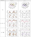 |
Figure 13. Bode diagram (modulus and phase) of the vocal tract HVT. The variation in the value of the ϕi parameters is studied in order to observe the changes in the transfer function. The errors |


6 Numerical experiments
In this section, we design a numerical testbed to test and examine the control of the trombone. Section 6.1 derives the numerical testbed. Section 6.2 presents the numerical experiments and discusses the results on the controller.
6.1 Numerical testbed
In the trombone modelling, we prioritise simplicity and ease of simulation in the discrete-time domain over incorporating the refinements (C1)–(C5) listed in Section 2.1, since the control law is independent of block A in Figure 2.
The trombone is decomposed into several passive components: a dissipative mouthpiece (described in Appendix A) and a trombone resonator composed of concatenated straight pipes (described in Appendix B). So that this approach yields a Kelly-Lochbaum structure like that used for the vocal tract system, because its passivity is preserved when it is discretized by bilinear transform.
All these steps are detailed in Appendix D and the full process is summarized in Figure 14.
![Mathematical equation: $$ {\hat {A}}(z) = \frac {1 + 2z^{-1} + z^{-2}}{\begin {array}{c}[Y_0 + 2f_s C_a + 2f_sY_0R_aC_a + 4f_s^2Y_0C_aM_a] \\ +\, z^{-1}[2Y_0 - 8Y_0f_s^2C_aM_a] \\ +\, z^{-2}[Y_0 - 2f_s C_a - 2f_sY_0R_aC_a + 4Y_0f_s^2C_aM_a]\end {array}} \ \ \ \ \ \ \ \ \ $$](/articles/aacus/full_html/2025/01/aacus240106/aacus240106-eq105.gif) (23a)
(23a)
![Mathematical equation: $$ {\hat {B}}(z) = \frac {\begin {array}{c}[Y_0 - 2f_sC_a + 2f_sY_0R_aC_a + 4f_s^2 Y_0 C_aM_a] \\ +\, z^{-1}[2Y_0 - 8Y_0f_s^2C_aM_a] \\ +\, z^{-2}[Y_0 + 2f_sC_a - 2f_sY_0R_aC_a + 4Y_0f_s^2C_aM_a]\end {array}}{\begin {array}{c}[Y_0 + 2f_s C_a + 2f_sY_0R_aC_a + 4f_s^2Y_0C_aM_a]\\ +\, z^{-1}[2Y_0 - 8Y_0f_s^2C_aM_a] \\ +\, z^{-2}[Y_0 - 2f_s C_a - 2f_sY_0R_aC_a + 4Y_0f_s^2C_aM_a]\end {array}} $$](/articles/aacus/full_html/2025/01/aacus240106/aacus240106-eq106.gif) (23b)
(23b)
![Mathematical equation: $$ {\hat {C}}(z) = \frac {2Y_0 + 4Y_0 z^{-1} + 2Y_0z^{-2}}{\begin {array}{c}[Y_0 + 2f_s C_a + 2f_sY_0R_aC_a + 4f_s^2Y_0C_aM_a]\\ +\, z^{-1}[2Y_0 - 8Y_0f_s^2C_aM_a]\\ +\, z^{-2}[Y_0 - 2f_s C_a - 2f_sY_0R_aC_a + 4Y_0f_s^2C_aM_a]\end {array}} $$](/articles/aacus/full_html/2025/01/aacus240106/aacus240106-eq107.gif) (23c)
(23c)
![Mathematical equation: $$ {\hat {D}}(z) = \frac {\begin {array}{c}[1 + R_aY_0 + 2f_sM_aY_0] \\ +\, z^{-1}[1 + 2R_aY_0] \\ +\, z^{-2}[1 + R_aY_0 - 2f_sM_aY_0]\end {array}}{\begin {array}{c}[Y_0 + 2f_s C_a + 2f_sY_0R_aC_a + 4f_s^2Y_0C_aM_a]\\ +\, z^{-1}[2Y_0 - 8Y_0f_s^2C_aM_a] \\ +\, z^{-2}[Y_0 - 2f_s C_a - 2f_sY_0R_aC_a + 4Y_0f_s^2C_aM_a]\end {array}} $$](/articles/aacus/full_html/2025/01/aacus240106/aacus240106-eq108.gif) (23d)
(23d)
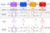 |
Figure 14. Description of the numerical testbed use for the trombone in the continuous and discrete time. Transfer functions A, B, C, D, T and R are given in equations X, from which transfer functions |


![Mathematical equation: $$ {\hat {R}}(z) = \frac {\begin {array}{c}[Z_c Y_2^c(2\alpha \kappa f_s + 4 \kappa ^2 f_s^2) - (1 + 4\xi \kappa f_s + 4 \kappa ^2 f_s^2)]\\ +\, z^{-1}[-8\kappa ^2f_s^2 Z_cY_2^c - (2 - 8 \kappa ^2 f_s^2)]\\ +\, z^{-2}[Z_cY_2^c (-2\alpha \kappa f_s + 4 \kappa ^2 f_s^2) - (1 - 4\xi \kappa f_s + 4 \kappa ^2 f_s^2)]\end {array}}{\begin {array}{c}[Z_cY_2^c(2\alpha \kappa f_s + 4\kappa ^2 f_s^2) + 1 + 4\xi \kappa f_s + 4 \kappa ^2 f_s^2]\\ +\, z^{-1}[-8 \kappa ^2 f_s^2 Z_cY_2^c + 2 - 8\kappa ^2f_s^2]\\ +\, z^{-2}[Z_cY_2^c (-2\alpha \kappa f_s + 4 \kappa ^2 f_s^2) + 1 - 4\xi \kappa f_s + 4\kappa ^2f_s^2]\end {array}} \ \ \ \ \ \ \ \ \ $$](/articles/aacus/full_html/2025/01/aacus240106/aacus240106-eq118.gif) (23e)
(23e)
![Mathematical equation: $$ {\hat {T}}(z) = Z_c\frac {\begin {array}{c}[4\alpha Y_2^c \kappa f_s + 8 Y_2^c \kappa ^2 f_s^2]\\ +\, z^{-1}[-16 Y_2^c \kappa ^2f_s^2]\\ +\, z^{-2}[-4\alpha Y_2^c\kappa f_s + 8Y_2^c \kappa ^2 f_s^2]\end {array}}{\begin {array}{c}[Z_cY_2^c(2\alpha \kappa f_s + 4\kappa ^2 f_s^2) + 1 + 4\xi \kappa f_s + 4 \kappa ^2 f_s^2]\\ +\, z^{-1}[-8 \kappa ^2 f_s^2 Z_cY_2^c + 2 - 8\kappa ^2f_s^2] + z^{-2}\\ {}[Z_cY_2^c (-2\alpha \kappa f_s + 4 \kappa ^2 f_s^2) + 1 - 4\xi \kappa f_s + 4\kappa ^2f_s^2]\end {array}}\cdot $$](/articles/aacus/full_html/2025/01/aacus240106/aacus240106-eq119.gif) (23f)
(23f)
6.2 Numerical experiments on the controller: results and discussion
Two numerical experiments are implemented, aiming at simulating the model of trombone described in Section 3 in the absence and in the presence of the model of controller described in Section 4. The first experiment aims to validate the operation of the control structure proposed in this paper and the expression of the controller model given in (19). To this end, a swept sine covering the frequency range of interest and sampled at 44.1 kHz is synthesised and used as the discrete-time mouthpiece flow  at the input of the trombone model. The outputs of the discrete-time model, namely the radiated pressure
  and the mouthpiece pressure
  are provided by the Kelly-Lochbaum representation of the trombone and the expressions
  ,
,  ,
,  ,
,  ,
,  and
and  defined in Figure 14 and given by (23a)–(23e). The numerical scheme is detailed in Appendix E. The
  component of the discrete-time radiated flowrate at the bell is then approximated by
  . In the presence of the controller, it is added to the
  component provided by the loudspeaker. Finally, the radiation impedance and the input impedance are estimated by the ratios of the discrete Fourier Transforms
  , and
, and  respectively. Figure 15 shows these ratios in the absence (left-hand column) and in the presence (right-hand column) of a controller.
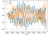 |
Figure 15. Transfer functions Hi=Zin,ZR in the Fourier domain, with (i=c) control and without (i=∅) control. The amplitude differences and frequency deviations of resonance peaks are noted in Table 5. |
In the absence of the controller (H∅): the estimate of Zin is similar to the trombone input impedance given in (C.2) and shown in Figure C.1. In particular, the first 5 peaks corresponding to the 5 lowest notes played on the trombone with the slide in first position (excluding the pedal note) are superimposed (see Tabs. 5 and C.1). As exposed in Appendix C, the Zin spectrum shows a decay of 20 dB per decade in the higher range, due to the mouthpiece acoustic compliance in parallel with the trombone resonator (see Appendix A). Then, the estimate of ZR, (see Fig. 15), is also similar to the radiation impedance model described in Section 3.1 and shown in Figure 9.
Comparison of the first five frequencies peaks Fk and amplitudes Ak of the first five peaks of the input impedance without control  and with control
  .
.
In the presence of the controller (Hc): Zin is slightly modified. As shown in Table 5, the first 5 resonance peaks are lowered in frequency, but by less than −1.12%, i.e. about one sixth of a semi-tone. The peak amplitudes are also modified, particularly in the vicinity of the formant frequencies, i.e. where HVT is large. Also, as expected, the spectral envelope of the radiation impedance ZR is close to the multiplication HVTZR. As a result, the presence of the controller has an effect on both the radiation and the input impedance of the trombone model. This means that the performer, while playing, should be able to feel the presence of the controller at the mouthpiece.
The second experiment aims to simulate the acoustic pressure in the mouthpiece and at the bell, in particular to listen to the controller effect on the sound of the trombone. For this purpose, the trombone model input is an acoustic flow waveform, extracted from previous measurements [35], with a duration of 184 ms and sampled at 44.1 kHz. The discrete-time acoustic pressure is calculated in the mouthpiece and at the bell using the Kelly-Lochbaum representation described in Figure D.1 in Appendix D. The vowel effect [a] applied to the trombone sound by active control can be appreciated by playing, listening and comparing the acoustic pressures Pin and Pout whose normalized waveforms are plotted in Figure 16. Their periods are similar, and approximately equal to 8.6 ms, which corresponds to a playing frequency of 116.28 Hz.
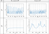 |
Figure 16. Normalized acoustic pressure waveforms in the trombone mouthpiece |


7 Conclusion
This analysis is a continuation of work begun previously [10]. By considering a simple but effective model of the instrument, the numerical results showed that it is possible to radiate a vowel through the trombone using active control. Sensitivity studies on the physical parameters and on the loudspeaker parameters allow us to envisage physical experiments.
Further studies will aim to develop a radiation-independent control, so that the control can be adapted to any playing situation. All the hypotheses cited above are discussed in perspective of an experimental realization: choice and co-location of microphones, pressure-to-voltage converter, loudspeakers.
The application of this work to a real trombone will be the object of a next publication.
This corresponds to a typical quality factor Q=10 for the first resonance of a straight pipe with the cross-section area 3 cm2 (approximate averaged value of cross-section area based on Fig. 8).
This means that the law is independent of the trombone configuration and the played note, but it is valid only for a static vowel.
Conflicts of interest
The authors declare that they have no conflicts of interest in relation to this article.
Data availability statement
The data are available from the corresponding author on request.
Appendix A Mouthpiece
The mouthpiece of a trombone is composed of two parts: a cavity (bowl) and a straight tube (tail). For wavelengths greater than its characteristic dimensions, the acoustic behaviour can be approximated by a lumped parameter model, as a Helmholtz resonator (see [36]): an acoustic compliance (Ca) for the bowl, in parallel with an acoustic mass-damper system (Ma,Ra) for the tail (see Fig. A.1 for an electronic analogy).
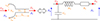 |
Figure A.1. Mouthpiece modelling. |
Parameters Ca, Ma and Ra are given by (see Tab. A.1 for typical values)
 (A.1)
(A.1)
where Vm is the volume of the bowl, rs and Ls are the radius and length of the tail and μ is the air viscosity (cf. [16]).
Numerical values chosen for the physical parameters of the mouthpiece. The radius rm and the length lm are based on the values of the Breslmair trombone models. The volume Vm is approximated to that of half an ellipsoid. The length value Ls is taken from Mignot [16]. The radius rs is approximated to be equal to rb for the sake of continuity.
Using the Kirchhoff's laws on the equivalent circuit yields, for all  ,
,
 (A.2a)
 (A.2b)
from which the deduced acoustic transfer relation is
![Mathematical equation: $$ \begin{aligned}&\mathop {\underbrace {\left [\begin {array}{ll} P_{\mathrm {in}}(s) \\ U_{\mathrm {in}}(s) \end {array}\right ]}}\limits _{X_{\mathrm {in}}(s)} \\ &\qquad = \mathop {\underbrace { \left [\begin {array}{ll} 1 & R_{\mathrm {a}} + s\,M_{\mathrm {a}} \\ s\,C_{\mathrm {a}}\; & 1 \!+\! s\, R_{\mathrm {a}}C_{\mathrm {a}}\!+\! s^2\, C_{\mathrm {a}}M_{\mathrm {a}} \end {array}\right ]}}\limits _{T_{\mathrm {a}}(s)} \, \mathop {\underbrace { \left [\begin {array}{ll} P_{0}(s) \\ U_{0}(s) \end {array}\right ]}}\limits _{X_0(s)}, \end{aligned} $$](/articles/aacus/full_html/2025/01/aacus240106/aacus240106-eq148.gif) (A.3)
(A.3)
and where matrix Ta takes the following concise form
![Mathematical equation: $$ T_{\mathrm {a}} =\left [\begin {array}{ll} 1 &\alpha \\ \beta &1 \!+\! \alpha \, \beta \end {array}\right ] \mathrm {\ with\ } \left\{ \begin {array}{ll} \alpha (s) &= R_{\mathrm {a}} + s\, M_{\mathrm {a}}, \\ \beta (s) &= s\,C_{\mathrm {a}}. \end {array} \right . $$](/articles/aacus/full_html/2025/01/aacus240106/aacus240106-eq149.gif) (A.4)
(A.4)
Appendix B Conservative bore and bell
This section describes the acoustic propagation in the bore and bell of the trombone, using a very simple model that is suitable for real-time simulations. The use of more refined models, in particular by considering viscothermal losses, see [37], is beyond the scope of this paper.
The pipe (straight and curved parts) is modelled by concatenating elementary 1D waveguides, so that it admits a Kelly-Lochbaum representation [30]. Although such representations are available for several piecewise-defined descriptions (e.g., conservative conical pipes [38], dissipative conical or curved pipes [16]), the choice adopted here for sake of simplicity is to concatenate elementary conservative straight pipes of length ln and cross-section area An, for 1≤n≤N (see Fig. B.1) localised for ℓ∈(Ln−1,Ln) with L0=0, and Ln=Ln−1+ln.
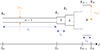 |
Figure B.1. Trombone modelling using concatenation of conservative straight pipes with L0=0 and Ln=Ln−1+ln, 1≤n≤N. |
The acoustics of each elementary cylinder n is described by its transfer matrix Tn(s) in the Laplace domain. It relates the acoustic states ![Mathematical equation: $ X_{n} = \left [\begin {array}{rr} P_{n}\\ U_{n} \end {array}\right ] $](/articles/aacus/full_html/2025/01/aacus240106/aacus240106-eq150.gif) at ℓ=Ln to Xn−1 at ℓ=Ln−1 as (see e.g., [39])
at ℓ=Ln to Xn−1 at ℓ=Ln−1 as (see e.g., [39])
![Mathematical equation: $$ \begin{aligned}X_{n-1} &= T_{n} X_{n} \\ \mathrm {\ with\ }T_{n}(s) &=\left [\begin {array}{rr} \cosh \frac {s l_{n}}{c_0} &\quad Z_{n} \sinh \frac {sl_{n}}{c_0}\\ Z_{n}^{-1} \sinh \frac {sl_{n}}{c_0} & \cosh \frac {sl_{n}}{c_0} \end {array}\right ] \end{aligned} $$](/articles/aacus/full_html/2025/01/aacus240106/aacus240106-eq151.gif) (B.1)
(B.1)
for all Laplace variable  , where Zn=ρ0c0/An and An denote the characteristic impedance and the cross section area of the nth cylinder respectively. The acoustics of the complete pipe is then described by
 (B.2)
(B.2)
the Kelly-Lochbaum structure of which is recalled below in Appendix D.
In a real trombone, the cylindrical bore is followed by the flare, almost conical part, and then the bell, more rapidly flaring part. Accordingly, in our model, the bore is modelled as a straight tube (n=1) with a constant cross section area equal to  , see Figure B.1. For the sake of simplicity, the flared part of the resonator hereafter called “the bell” is composed of a succession of Nbell short straight tubes subsequently called segments of equal length d.
Note that for the following simulations: (i) d is chosen so that the propagation time in each tube is half a sampling period [14]; (ii) the length of the bore l1 is a multiple of d. In addition, the tubes radii in the resonator are chosen such that their rate of increase along the bore exceeds −13.64%, minimum spatial derivative of the radius reported in [40] on a measured trombone bore profile (Courtois TB 14, France).
These parameters result from an optimisation procedure [41], which minimises the distance between the input impedance peaks 2 to 6 of our model (Fk,k∈ [6, 40]), to those of a real bass trombone (Fk,k∈ [6, 40]) with the slide in first position, measured in a previous study [35] (Yamaha YBL 321, Hamamatsu, Japan). The optimisation criterion does not concern the first impedance peak, which is generally not played because its harmonics do not coincide with the following peaks.
Table B.1 gives the numerical values of the above-mentioned physical parameters of the resonator. The resulting profile of the bell is shown in Figure B.2: the 450 segments of equal length d verifying the relationship lbell=450·d are represented. Their radii take on 15 different values, each repeated 30 times to facilitate optimisation. Radius values are reported in Table B.2.
 |
Figure B.2. Profile of the bell. |
Characteristics of the trombone resonator used for simulation. These values are taken from the optimisation calculation [41], see Appendix F.
Comparison of the values of the 15 radius Rk and their rate of increase. As shown in Figure B.2, the radius profile increases overall. A previous measurement [40] report a comparable radius profile, ranging from 6.9 mm to 101.8 mm with a rate of increase, that can be negative, but always bigger than −13.64%.
Appendix C Global transfer functions
Assembling the mouthpiece (Ta), the pipe (Tpipe) and the radiation load (ZR) leads to the transfer relation (denoting ![Mathematical equation: $ X_{\mathrm {out}}= \left [\begin {array}{l} P_{\mathrm {out}} \\ U_{\mathrm {out}} \end {array}\right ] =X_{N} $](/articles/aacus/full_html/2025/01/aacus240106/aacus240106-eq157.gif) ), from (B.2) and (A.3):
), from (B.2) and (A.3):
 (B.1a)
![Mathematical equation: $$ \mathrm {\ with\ } T_{\mathrm {tbn}} = T_{\mathrm {a}} \,T_{\mathrm {pipe}} \mathrm {\ and\ } X_{\mathrm {out}} = \left [\begin {array}{l} Z_{\mathrm {R}} \\ 1 \end {array}\right ] U_{\mathrm {out}}. $$](/articles/aacus/full_html/2025/01/aacus240106/aacus240106-eq159.gif) (C.1b)
(C.1b)
The input impedance Zin=Pin/Uin is then given by
 (C.2)
(C.2)
Figure C.1 compares Zin with the measured input impedance  of the real bass trombone considered for the optimisation in Section B (see [35]).
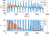 |
Figure C.1. Modulus (top) and phase (bottom) of measured (red) and modelled (blue) trombone input impedance. The mouthpiece effect appears in the higher frequency range, when the modulus tends to −20 dB/dec asymptotic curve (green) and the phase tends to −π/2. |
It appears that the Q-factors of the resonances are greater in Zin than in  , as the model does not take viscothermal losses into account. Above the cut-off frequency, the impact of mouthpiece compliance on the input impedance is therefore lower in the model than in the measurement. This explains why the resonance Q-factors are greater in the model, even in the higher frequency range.
Table C.1 presents the amplitude and frequency differences of peaks 2 to 6 between the model Zin and the measurement  .
.
Comparison of the frequencies Fk and amplitudes Ak of the first five peaks  and Zin.
Appendix D Kelly-Lochbaum structure
The Kelly-Lochbaum structure governs travelling wave variables. Consider the nth elementary straight pipe with characteristic impedance  . The travelling wave signals at its left side are
  , those at its right side are
  , and they are related by a pure delay, called Dn (see Fig. D.1):
![Mathematical equation: $$ \left [\begin {array}{r} P_{n}^{\mathrm {r}+}\\ P_{n}^{\mathrm {l}-} \end {array}\right ] = D_{n} \, \left [\begin {array}{r} P_{\mathrm {n}}^{\mathrm {l}+}\\ P_{\mathrm {n}}^{\mathrm {r}-} \end {array}\right ] \mathrm {\ with\ } D_{\mathrm {n}}(s) = \mathrm {e}^{-\frac {s\,d}{2c}}. $$](/articles/aacus/full_html/2025/01/aacus240106/aacus240106-eq174.gif) (D.1)
(D.1)
Between pipes n and n+1, expressing  and
and  as functions of
  and
and  yields the structure of junction Jn detailed in Figure D.1 and involved in Figure 14, where the constant reflection coefficients kn are
 (D.2)
(D.2)
At the trombone input, the relation between Xin and  is described by
![Mathematical equation: $$ \mathop {\underbrace {{\left [\begin {array}{c} P_{\mathrm {in}}\\ U_{\mathrm {in}} \end {array}\right ]}}}\limits _{X_{\mathrm {in}}} = T_{\mathrm {a}} {\left [\begin {array}{c} P_0\\ U_0 \end {array}\right ]} = \mathop {\underbrace {T_{\mathrm {a}} {\left [\begin {array}{cc} 1 & 1\\ Y_1 & -Y_1 \end {array}\right ]}}}\limits _{M} {\left [\begin {array}{c} P_1^{\mathrm {l}+}\\ P_1^{\mathrm {l}-} \end {array}\right ]}, $$](/articles/aacus/full_html/2025/01/aacus240106/aacus240106-eq181.gif) (D.3)
(D.3)
with, from (A.3),
![Mathematical equation: $$ M = {\left [\begin {array}{cc} 1 + \alpha Y_1 & 1 - \alpha Y_1\\ \beta + (1 + \alpha \beta )Y_1 & \beta - (1 + \alpha \beta )Y_1\end {array}\right ]}. $$](/articles/aacus/full_html/2025/01/aacus240106/aacus240106-eq182.gif) (D.4)
(D.4)
The transfer functions A, B, C, D involved in Figure 14 are derived from the elements of M, by expressing Pin and  as functions of Uin and
  . Computations yield:
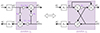 |
Figure D.1. Kelly-Lochbaum structure of a segment, composed of two delays Dn(s), and a junction Jn, that governs travelling wave signals (see Appendix E for detailed computations). On the left: the schematic diagram of the junction; on the right: the equivalent way in which the junction is implemented. |
 (D.5)
(D.5)
the detailed expressions of which are given in the left-hand column of Table D.1.
Expressions of the transfer functions A,B,Cand D defined in (D.5) for the mouthpiece (left-hand column) and the vocal tract (right-hand column). These transfer functions give the pressure travelling waves at the inlet to the first tube of the Kelly-Lochbaum structure in Figure 14, with respect to the input pressure and flow.
At the trombone output, PN=ZRUN so that signals  equal (ZRUN±ZNUN)/2. Then, the reflection function
  in Figure 14 is given by
 (D.6a)
which is similar to (D.2) but not constant, and the transmission function  is given by
 (D.6b)
Appendix E Coefficient relations
We note the demonstration of the coefficient relations exposed in Figure D.1. Pressure in nth segment Pn is computed from the left-progressive one of the (n+1)th segment noted  and from the left-regressive one of the (n+1)th segment noted
  . Flow rate is deduced thanks to the impedance relation. We obtain:
 (E.1)
(E.1)
The same relation can be exposed on the right-side of the segment,
 (E.2)
(E.2)
Using (E.1) and (E.2), we can express  as a function of
  and
and  ,
,
by regrouping the following terms,
As a result, a kn coefficient is expressed,
 (E.3)
(E.3)
with  .
.
Appendix F Optimisation
The length of the resonator Ltot is chosen to fix the first harmonic peak at 37 Hz. As an open/close pipe, its resonance frequencies follow the relation fp=(2p+1)  . The length of a straight pipe is equal to d (see Sect. 3.2). So, the number of straight pipes must be equal to 560.6, approximating to Ntot=561 (this approximation gives f1=111.92 Hz, which corresponds to a relative error of 0.018%). As Ntot, Nbell must be an integer, i.e.,
  . Moreover, the optimisation algorithm is based on a target of a 15-radius model. For this reason, Nbell must therefore be an integer and a multiple of 15. These conditions led us to choose Nbell=30×15=450. Table F.1 summarises the values chosen to the algorithmic optimisation.
List of the chosen parameters for simulations. The choices of Lbell and Nbore are explained below.
References
- L. Paul: Process of silencing sound oscillations. US Patent 2,043,416, June 9 1936 [Google Scholar]
- L.J. Fogel: Apparatus for improving intelligence under high ambient noise levels. US Patent 2,966,549, December 27 1960 [Google Scholar]
- D. Crombie: Piano: Evolution, Design and Performance. Barnes and Noble Books, New York, 1995 [Google Scholar]
- G.S. Heet: String instrument vibration initiator and sustainer. The Journal of the Acoustical Society of America 65, 6 (1979) 1609–1609 [Google Scholar]
- G. T Osborne, A. A Hoover: Sustainer for a musical instrument. US Patent 5,932,827, August 3 1999 [Google Scholar]
- H. Boutin: Méthodes de contrôle actif d’instruments de musique. Cas de la lame de xylophone et du violon. PhD thesis, UPMC-Université Paris 6 Pierre et Marie Curie, 2011 [Google Scholar]
- T. Meurisse: Contrôle actif appliqué aux instruments de musique à vent. PhD thesis, Paris 6, 2014 [Google Scholar]
- C. Maganza, R. Caussé, F. Laloë: Bifurcations, period doublings and chaos in clarinetlike systems. Europhysics Letters 1, 6 (1986) 295 [CrossRef] [Google Scholar]
- J. S Lienard: An overview of speech synthesis, in: Spoken Language Generation and Understanding: Proceedings of the NATO Advanced Study Institute held at Bonas, France, June 26–July 7, 1979. Springer, 1980, pp. 397–412. See also 〈hal-04424757〉 from the same author and coll [Google Scholar]
- V. Martos, H. Boutin, T. Hélie, B. d’Andréa Novel: Radiation impedance control of brass resonators to reshape sounds with vowel spectral envelopes: a numerical study, in: Forum Acusticum 2023: The 10th Convention of the European Acoustics Association, 2023 [Google Scholar]
- C. Vergez: Trompette et trompettiste: un système dynamique non linéaire à analyser, modéliser et simuler dans un contexte musical. PhD thesis, Paris 6, 2000 [Google Scholar]
- N. Lopes: Approche passive pour la modélisation, la simulation et l’étude d’un banc de test robotisé pour les instruments de type cuivre. PhD thesis, Université Paris 6 (UPMC), 2016 [Google Scholar]
- J.D. Polack: Time-domain solution of Kirchhoff's equation for sound propagation in viscothermal gases: a diffusion process. Journal d’acoustique (Les Ulis) 4 (1991) 47–67 [Google Scholar]
- D. Matignon: Représentations en variables d’état de modèles de guides d’ondes avec dérivation fractionnaire. PhD thesis, Paris 11, 1994 [Google Scholar]
- T. Hélie: Modélisaiton physique d’instruments de musique en système dynamique et inversion. PhD thesis, Paris 11, 2002 [Google Scholar]
- R. Mignot: Réalisation en guides d’ondes numériques stables d’un modèle acoustique réaliste pour la simulation en temps-réel d’instruments à vent. PhD thesis, Télécom ParisTech, 2009 [Google Scholar]
- A. Thibault: Modélisation, analyse et simulation de l’acoustique dissipative dans les tubes poreux ou rugueux: application aux instruments à vent. PhD thesis, Pau, 2023 [Google Scholar]
- N. Amir, V. Pagneux, J. Kergomard: A study of wave propagation in varying cross-section waveguides by modal decomposition. Part II. Results. The Journal of the Acoustical Society of America 101, 5 (1997) 2504–2517 [Google Scholar]
- L. Menguy, J. Gilbert: Weakly nonlinear gas oscillations in air-filled tubes; solutions and experiments. Acta Acustica United with Acustica 86, 5 (2000) 798–810 [Google Scholar]
- R. Msallam, S. Dequidt, R. Causse, S. Tassart: Physical model of the trombone including nonlinear effects. Application to the sound synthesis of loud tones. Acta Acustica United with Acustica 86, 4 (2000) 725–736 [Google Scholar]
- T. Hélie, V. Smet: Simulation of the weakly nonlinear propagation in a straight pipe: application to a real-time brassy audio effect, in: 2008 16th Mediterranean Conference on Control and Automation. IEEE, 2008, pp. 1580–1585 [Google Scholar]
- M. Campbell, J. Gilbert, M. Arnold: The Science of Brass Instruments. Vol. 436. Springer, 2021 [Google Scholar]
- A.P. McPherson: Techniques and circuits for electromagnetic instrument actuation, in: NIME. London, 2012 [Google Scholar]
- J.P. Dalmont, C. J Nederveen, N. Joly: Radiation impedance of tubes with different flanges: numerical and experimental investigations. Journal of Sound and Vibration 244, 3 (2001) 505–534 [CrossRef] [Google Scholar]
- F. Silva, P. Guillemain, J. Kergomard, B. Mallaroni, A.N. Norris: Approximation formulae for the acoustic radiation impedance of a cylindrical pipe. Journal of Sound and Vibration 322, 1–2 (2009) 255–263 [CrossRef] [Google Scholar]
- T. Hélie: Modélisation physique d’instruments de musique et de la voix: systèmes dynamiques, problèmes directs et inverses. Habilitation à Diriger des Recherches, 2013, pp. 42–43 [Google Scholar]
- P. Eveno, J.P. Dalmont, R. Caussé, J. Gilbert: Wave propagation and radiation in a horn: comparisons between models and measurements. Acta Acustica United with Acustica 98, 1 (2012) 158–165 [Google Scholar]
- T. Hélie, T. Hézard, R. Mignot, D. Matignon: One-dimensional acoustic models of horns and comparison with measurements. Acta acustica United with Acustica 99, 6 (2013) 960–974 [Google Scholar]
- S. Mathur, B.H. Story: Vocal tract modeling: implementation of continuous length variations in a half-sample delay Kelly-Lochbaum model, in: Proceedings of the 3rd IEEE International Symposium on Signal Processing and Information Technology (IEEE Cat. No. 03EX795). IEEE, 2003, pp. 753–756 [Google Scholar]
- J.L. Kelly, C.C. Lochbaum: Speech synthesis, in: Proc. 4th Int. Congr. Acoustics, Sep. 1962, pp. 1–4 [Google Scholar]
- B.H. Story, I.R. Titze, E.A. Hoffman: Vocal tract area functions from magnetic resonance imaging. The Journal of the Acoustical Society of America 100, 1 (1996) 537–554 [Google Scholar]
- H. Boutin, J. Smith, J. Wolfe: Warming up a wind instrument: the time-dependent effects of exhaled air on the resonances of a trombone. The Journal of the Acoustical Society of America 148, 4 (2020) 1817–1823 [Google Scholar]
- N. Thiele: Loudspeakers in vented boxes: Part 1. Journal of the Audio Engineering Society 19, 5 (1971) 382–392 [Google Scholar]
- R.H. Small: Closed-box loudspeaker systems-part 1: analysis. Journal of the Audio Engineering Society 20 (1972) 798–808 [Google Scholar]
- H. Boutin, N. Fletcher, J. Smith, J. Wolfe, Relationships between pressure, flow, lip motion, and upstream and downstream impedances for the trombone. The Journal of the Acoustical Society of America 137, 3 (2015) 1195–1209 [Google Scholar]
- M.S. Howe: On the helmholtz resonator. Journal of Sound and Vibration 45, 3 (1976) 427–440 [Google Scholar]
- A. Thibault, J. Chabassier: Dissipative time-domain one-dimensional model for viscothermal acoustic propagation in wind instruments. The Journal of the Acoustical Society of America 150, 2 (2021) 1165–1175 [Google Scholar]
- V. Välimäki, M. Karjalainen: Improving the Kelly-Lochbaum vocal tract model using conical tube sections and fractional delay filtering techniques, in: ICSLP, 1994 [Google Scholar]
- A. Chaigne: Ondes acoustiques. Editions Ecole Polytechnique, 2001 [Google Scholar]
- R. Caussé, J. Kergomard, X. Lurton: Input impedance of brass musical instruments – comparison between experiment and numerical models. The Journal of the Acoustical Society of America 75, 1 (1984) 241–254 [Google Scholar]
- J.C. Lagarias, J.A. Reeds, M.H. Wright, P.E. Wright: Convergence properties of the nelder-mead simplex method in low dimensions. SIAM Journal of Optimization 9, 1 (1998) 112–147 [CrossRef] [Google Scholar]
Cite this article as: Martos V. Boutin H. Hélie T. & d’Andréa-Novel B. 2025. Electro-acoustic control of radiation impedance for brass instrument timbre shaping: design of a vocalizing mute. Acta Acustica, 9, 40. https://doi.org/10.1051/aacus/2025020.
All Tables
Comparison of the frequencies Fk and amplitudes Ak of the first five peaks of H† and Herr.
Physical, Thiele and Small and reduced parameters of the speaker SICA 3L 0.8 SL 8Ω mode Z000900, given by the manufacturer. Note: Greyed-out parameters in the first 2 lines are not used in the expression of the controller K, because it is designed to control the loudspeaker in current.
Comparison of the first five frequencies peaks Fk and amplitudes Ak of the first five peaks of the input impedance without control and with control .
Numerical values chosen for the physical parameters of the mouthpiece. The radius rm and the length lm are based on the values of the Breslmair trombone models. The volume Vm is approximated to that of half an ellipsoid. The length value Ls is taken from Mignot [16]. The radius rs is approximated to be equal to rb for the sake of continuity.
Characteristics of the trombone resonator used for simulation. These values are taken from the optimisation calculation [41], see Appendix F.
Comparison of the values of the 15 radius Rk and their rate of increase. As shown in Figure B.2, the radius profile increases overall. A previous measurement [40] report a comparable radius profile, ranging from 6.9 mm to 101.8 mm with a rate of increase, that can be negative, but always bigger than −13.64%.
Comparison of the frequencies Fk and amplitudes Ak of the first five peaks and Zin.
Expressions of the transfer functions A,B,Cand D defined in (D.5) for the mouthpiece (left-hand column) and the vocal tract (right-hand column). These transfer functions give the pressure travelling waves at the inlet to the first tube of the Kelly-Lochbaum structure in Figure 14, with respect to the input pressure and flow.
List of the chosen parameters for simulations. The choices of Lbell and Nbore are explained below.
All Figures
|
Figure 1. Block diagram of a played trombone in its environment. First, the pipe is described by a quadripole. The two inputs are the mouthpiece volumetric flow rate, denoted Uin and the pressure at the bell, denoted P. The two outputs are the flow rate at the bell, Utb and the mouthpiece pressure Pin. Second, the radiation is represented by a linear impedance load ZR (equal to P/Utb in the Laplace domain). And the transfer impedance TR(r) between Utb and the pressure Pout(r) at a point r. Note that in all the paper, flow rates are algebraic quantities counted positively in the direction of eℓ (e.g., Uin=Uineℓ). |
| In the text | |
|
Figure 2. Block diagram of the musical instrument equipped with active control. Note that with no control (Uac=0), we recover the Figure 1 (UR=Utb). |
| In the text | |
|
Figure 3. Block diagram in the Laplace domain of the overall control structure. It is composed of a microphone (transfer function between acoustic pressure P and voltage Vmicro), a controller (cascaded transfer functions K and Ampli between voltage Vmicro) and current ILS and a loudspeaker LS (quadripole with two inputs – pressure P and current ILS – and two outputs – voltage VLS and flow rate Uac). |
| In the text | |
|
Figure 4. Radiation model of the bell of a wind instrument. The purple spherical cap S0 is the uniformly animated part and the orange cap S−S0 is motionless (see details in [26]). |
| In the text | |
|
Figure 5. Bode diagram of adimensioned radiation impedance |
| In the text | |
|
Figure 6. Modelling the vocal tract. |
| In the text | |
|
Figure 7. Bode diagram of the transfer function HVT(s=2iπf) of a vocal tract for the vowel profile [a] (see Fig. 8), loaded by |
| In the text | |
|
Figure 8. Area profile of the vocal tract for vowel [a] extracted from [31, Table 3] (NVT=44 cascaded pipes, total length LVT=17.46 cm, so that LVT/NVT=3.968 mm). |
| In the text | |
|
Figure 9. Block diagram of the target radiation impedance in the Laplace domain. Here, the vocal tract HVT is placed between the pipe and the radiation such that the new radiation flow rate UR is now equal to UR=HVTUtb. |
| In the text | |
|
Figure 10. Bode diagrams: (a) radiation impedances |
| In the text | |
|
Figure 11. Bode diagrams: (a) vocal tract filters H† (exact, in red) and Herr (erroneous, in blue); (b) error characterisation. (a) vocal tract filters: (top) modulus in dB; (bottom) phase in radians. (b) error: (top) relative error modulus |ϵH| (log scale); (bottom) phase deviation Δϕ=ϕerr−ϕ†. |
| In the text | |
|
Figure 12. Bode diagram (modulus and phase) of the vocal tract filter HVT. The variation in the value of the ai parameters is studied in order to observe the changes in the transfer function. The errors |
| In the text | |
|
Figure 13. Bode diagram (modulus and phase) of the vocal tract HVT. The variation in the value of the ϕi parameters is studied in order to observe the changes in the transfer function. The errors |
| In the text | |
|
Figure 14. Description of the numerical testbed use for the trombone in the continuous and discrete time. Transfer functions A, B, C, D, T and R are given in equations X, from which transfer functions |
| In the text | |
|
Figure 15. Transfer functions Hi=Zin,ZR in the Fourier domain, with (i=c) control and without (i=∅) control. The amplitude differences and frequency deviations of resonance peaks are noted in Table 5. |
| In the text | |
|
Figure 16. Normalized acoustic pressure waveforms in the trombone mouthpiece |
| In the text | |
|
Figure A.1. Mouthpiece modelling. |
| In the text | |
|
Figure B.1. Trombone modelling using concatenation of conservative straight pipes with L0=0 and Ln=Ln−1+ln, 1≤n≤N. |
| In the text | |
|
Figure B.2. Profile of the bell. |
| In the text | |
|
Figure C.1. Modulus (top) and phase (bottom) of measured (red) and modelled (blue) trombone input impedance. The mouthpiece effect appears in the higher frequency range, when the modulus tends to −20 dB/dec asymptotic curve (green) and the phase tends to −π/2. |
| In the text | |
|
Figure D.1. Kelly-Lochbaum structure of a segment, composed of two delays Dn(s), and a junction Jn, that governs travelling wave signals (see Appendix E for detailed computations). On the left: the schematic diagram of the junction; on the right: the equivalent way in which the junction is implemented. |
| In the text | |
Current usage metrics show cumulative count of Article Views (full-text article views including HTML views, PDF and ePub downloads, according to the available data) and Abstracts Views on Vision4Press platform.
Data correspond to usage on the plateform after 2015. The current usage metrics is available 48-96 hours after online publication and is updated daily on week days.
Initial download of the metrics may take a while.