© The Author(s), Published by EDP Sciences, 2026

1 Introduction

Ultrasounds are widely used to image fluid and solid media. The produced image is expected to allow the visualization in space of either the variations of the mechanical properties of the medium being probed, or of the location and shape of defects (such as holes, cracks or delaminations) that may be present. Numerous active techniques exist, all based on two principles. First, one or several transducers emit waves that propagate in the inspected structure and are received by the same or other transducers, to give the response of the structure. Then, the image is computed from the emitted and received signals based on a model of the wave propagation in the inspected medium, whose choice may reflect a compromise between accuracy and computational cost. Classical well-established methods are based on the delay-and-sum principle which assumes a globally homogeneous semi-infinite medium. The underlying heuristics is as follows: an heterogeneity located at given coordinates produces an acoustic signature in the measured signals at a time corresponding to the wave propagation from emitters to the heterogeneity and back to the receiver. The intensity associated to each pixel is typically defined as the sum of each signal delayed by this back and forth propagation duration [1]. This principle allows efficient and detailed imaging for medical and non destructive testing (NDT) purposes using transducer arrays when the investigated regions are accessible with a direct wave path. As such methods cannot process multiply reflected waves, regions that are masked by the structure geometry cannot be investigated. Such difficulties may be addressed with the help of more general imaging heuristics arising from the inverse problem community.

Quantitative medium imaging is often based on the minimization of a misfit functional that quantifies the distance between experimental measurements and their model predictions for a given trial medium. The latter is modified at each iteration following a descent direction defined in terms of the Fréchet derivative of the misfit functional. The latter can be computed by various methods introduced for inverse problems in geophysics (where in particular the migration principle of Claerbout [2] was recast [3, 4] as a local optimization problem) and many other areas [5]. An efficient evaluation of the misfit gradient usually relies on an adjoint solution approach, that can be seen as a particular case of the general adjoint-state method (reviewed in [6]) used in PDE-constrained optimization, where a Lagrangian is introduced as an augmented misfit functional (e.g. [7]). Full waveform inversion (FWI) algorithms [8, 9] then use the minimization for mapping the space-dependent mechanical properties of the medium. Such algorithms exist in many forms, including one based on the error in constitutive relation [10] and applied to wave-based elasticity imaging from full-field measurements [11].

The fact that optimization-based quantitative medium imaging is computation-intensive elicits the formulation of faster alternatives that achieve qualitative medium imaging. This work aims at proposing one such approach, which exploits the Fréchet derivative at the reference material of a misfit functional designed to emphasize early reverberations. Alternative imaging approaches belonging to the same general family exploit the concept of topological derivative, which was initially developed [12] for finding optimal structures subjected to static loads via topological optimization. This concept was extended in [13] to address the inverse problem of imaging inclusions in a structure interrogated with elastic waves. The exact expression of the relevant (Fréchet or topological) derivative depends on the choice of misfit functional and on the kind of mechanical property (for FWI) or of inclusions (for topological optimization) to be mapped. Still, all such derivatives can be expressed relatively simply, as bilinear functionals on the direct and adjoint problem solutions defined for the current reference medium. In addition to optimization-based imaging methods, qualitative imaging methods based on linear sampling or factorization ideas are also available, see e.g. [14] for elastodynamic media and references therein; they however are not well suited to the present context as they require abundant data (multiple sources and full aperture observations).

The absence of restrictive hypotheses for the initial reference medium and the physical interpretation of the adjoint problem as a time-reversal process [15] confer to this approach a strong potential for imaging complex media. Initial attempts at non-iterative imaging applications were performed for non-destructive testing [16, 17] using a simple homogeneous semi-infinite reference medium. An experimental application to a bounded reverberating medium [18] demonstrates that locating accurately a masked defect is possible and that the topological imaging method takes full advantage of reverberation as a single transducer is used. Still, this approach cannot be used without modifications for realistic applications, as the system is not only sensitive to the presence of defects but also to environmental conditions such as temperature or boundary condition perturbations. To mitigate the latter issue, a first attempt at truncating reverberation was numerically evaluated for rail inspection [19]. While producing interesting results, the truncation approach used therein was not consistent with the theoretical background of the method. In this work, we define a reverberation-truncation approach that is incorporated directly in the equations governing elastic wave propagation and the misfit functional defining the inverse problem of imaging local mechanical parameter variations, making the whole approach fully consistent with the elastodynamic propagation model for solids of arbitrary shapes. This lays the foundations of an imaging method for elastic confined media, whose potential is demonstrated here on a simple two-dimensional test case. More-comprehensive explorations of the many possibilities opened by the proposed approach are left to follow-up work.

The remainder of this paper consists of two main parts. First, we develop in Section 2 the proposed finite-duration imaging methodology and outline its implementation. We then assess in Section 3 the potential of our approach using computational experiments on a two-dimensional test case. The paper closes with concluding remarks (Sect. 4).

2 Formulation of finite-duration imaging functions

2.1 Standard equations for propagation in an elastic bounded domain

In an elastic bounded domain Ω containing no source, Newton’s second law and Hooke’s law are written as follows:

$$\begin{array}{c}\hfill \forall \mathbf{x}\in \mathrm{\Omega },\forall t>0\text{,}\rho (\mathbf{x}){\partial }_t^2\underline{\mathbf{u}}(\mathbf{x},t)=\mathrm{\nabla }·\underline{\mathrm{\Sigma }}(\mathbf{x},t)\end{array}$$(1)

and

$$\begin{array}{c}\hfill \underline{\mathrm{\Sigma }}(\mathbf{x},t)=\mathcal{C}(\mathbf{x}):\mathrm{\nabla }\underline{\mathbf{u}}(\mathbf{x},t),\end{array}$$(2)

where the displacement vector and the stress tensor at time t and position x are denoted by $\underline{\mathbf{u}}$ and $\underline{\mathrm{\Sigma }}$, respectively. The mass density ρ and the elastic stiffness tensor 𝒞 depend on the position but not on time.

The elastic waves propagating in the domain Ω are generated by sources located on its boundary ∂Ω and characterized by a surface force $\underline{\mathbf{f}}(\mathbf{x},t)$:

$$\begin{array}{c}\hfill \forall \mathbf{x}\in \partial \mathrm{\Omega }\text{,}\forall t>0,\underline{\mathrm{\Sigma }}(\mathbf{x},t)\mathbf{n}(\mathbf{x})=\underline{\mathbf{f}}(\mathbf{x},t),\end{array}$$(3)

where n(x) denotes the outward unit vector normal to the boundary. Other types of excitations could be considered instead with minor modifications. Finally, initial-rest conditions are assumed:

$$\begin{array}{c}\hfill \underline{\mathbf{u}}(\mathbf{x},0)={\partial }_t\underline{\mathbf{u}}(\mathbf{x},0)=\mathbf{0}.\end{array}$$

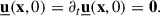
2.2 Introduction of windowed signals

Since the domain is (by assumption) bounded and lossless, any excitation, no matter how short, will generate a response of infinite duration. Such signal cannot be processed in a standard way by discrete Fourier transform. For this reason, we choose to work on signals windowed by a decreasing exponential window, as previously done e.g. in [20–22]. This technique is generally referred to in the literature as the Exponential Window Method (EWM). Indeed, these windowed signals are in practice of finite duration, contrary to physical signals which oscillate indefinitely with little or no attenuation.

Accordingly, we introduce the windowed displacement vector u defined in terms of the physical displacement $\underline{\mathbf{u}}$ by

$$\begin{array}{c}\hfill \mathbf{u}(\mathbf{x},t)=exp(-\gamma t)\underline{\mathbf{u}}(\mathbf{x},t),\end{array}$$(4)

such that the Fourier transform of the function t ↦ u(x, t) coincides with the restriction of the Laplace transform of $t\mapsto \underline{\mathbf{u}}(\mathbf{x},t)$ to a vertical line of equation ℜ(s)=γ in the complex s-plane. This latter point is crucial for numerical computations in the frequency domain by means of either by integral transforms in multilayer canonical structures [22, 23] or the Finite Element Method in lossless domains, as described below. Windowed versions of other quantities, e.g. Σ, are defined in the same manner. Definition (4) implies that $\underline{\mathbf{u}}$ and its time derivatives are given in terms of u by

$$\begin{array}{c}\hfill \begin{array}{cc}\hfill \underline{\mathbf{u}}(\mathbf{x},t)& =exp(\gamma t)\mathbf{u}(\mathbf{x},t),\hfill \\ \hfill {\partial }_t\underline{\mathbf{u}}(\mathbf{x},t)& =exp(\gamma t)({\partial }_t+\gamma )\mathbf{u}(\mathbf{x},t),\hfill \\ \hfill {\partial }_t^2\underline{\mathbf{u}}(\mathbf{x},t)& =exp(\gamma t)({\partial }_t^2+2\gamma {\partial }_t+{\gamma }^2)\mathbf{u}(\mathbf{x},t),\hfill \end{array}\end{array}$$(5)

and similarly for all windowed fields. The duration T and the parameter γ are set as explained in Section 3.4.1; in particular they are inversely proportional to each other and such that exp(γ T) is small enough.

2.3 Forward problem

2.3.1 Standard form of the equations satisfied by the windowed fields

By using relations (5), Newton’s second law (1) and Hooke’s law (2) become for the windowed displacement vector u and the windowed stress tensor Σ:

$$\begin{array}{cc}& \forall \mathbf{x}\in \mathrm{\Omega },\forall t>0,\hfill \\ \hfill & \rho (\mathbf{x})({\partial }_t^2+2\gamma {\partial }_t+{\gamma }^2)\mathbf{u}(\mathbf{x},t)=\mathrm{\nabla }·\mathrm{\Sigma }(\mathbf{x},t)\hfill \\ \hfill \text{and}& \mathrm{\Sigma }(\mathbf{x},t)=\mathcal{C}(\mathbf{x}):\mathrm{\nabla }\mathbf{u}(\mathbf{x},t),\hfill \end{array}$$

so that u satisfies the following wave equation:

$$\begin{array}{cc}\hfill \forall \mathbf{x}\in \mathrm{\Omega },\forall t>0,\rho (\mathbf{x})& ({\partial }_t^2+2\gamma {\partial }_t+{\gamma }^2)\mathbf{u}(\mathbf{x},t)\hfill \\ \hfill & -\mathrm{\nabla }·[\mathcal{C}(\mathbf{x}):\mathrm{\nabla }\mathbf{u}(\mathbf{x},t)]=0.\hfill \end{array}$$(6)

In addition, the windowed fields obey the boundary condition

$$\begin{array}{c}\hfill \forall \mathbf{x}\in \partial \mathrm{\Omega },\forall t>0,\mathrm{\Sigma }(\mathbf{x},t)\mathbf{n}(\mathbf{x})=\mathbf{f}(\mathbf{x},t),\end{array}$$(7)

arising from (3), where f denotes the windowed surface force, and the initial-rest conditions

$$\begin{array}{c}\hfill \forall \mathbf{x}\in \mathrm{\Omega },\mathbf{u}(\mathbf{x},0)={\partial }_t\mathbf{u}(\mathbf{x},0)=\mathbf{0}.\end{array}$$

2.3.2 Weak form of the wave equation

The wave equation (6) and boundary condition (7) can be gathered into a single equation, namely the weak form of the forward problem, which is perfectly adapted to both the imaging formalism and finite element methods, as follows: for any test function w, we have

$$\begin{array}{c}\begin{array}{l}\mathrm{\forall }t>0,\\ {\int }_{\mathrm{\Omega }}\rho (\mathbf{x})\mathbf{w}(\mathbf{x})\cdot ({\mathrm{\partial }}_t^2+2\gamma {\mathrm{\partial }}_t+{\gamma }^2)\mathbf{u}(\mathbf{x},t)\mathbb{d}\mathbf{x}\\ -{\int }_{\mathrm{\Omega }}\mathrm{\nabla }\mathbf{w}(\mathbf{x}):\mathcal{C}(\mathbf{x}):\mathrm{\nabla }\mathbf{u}(\mathbf{x},t)\mathbb{d}\mathbf{x}\\ ={\int }_{\mathrm{\partial }\mathrm{\Omega }}\mathbf{w}(\mathbf{x})\cdot \mathbf{f}(\mathbf{x},t)d\mathbf{x},\\ \mathrm{\forall }\mathbf{x}\in \mathrm{\Omega },\mathbf{u}(\mathbf{x},0)={\mathrm{\partial }}_t\mathbf{u}(\mathbf{x},0)=\mathbf{0}.\end{array}\}\end{array}$$(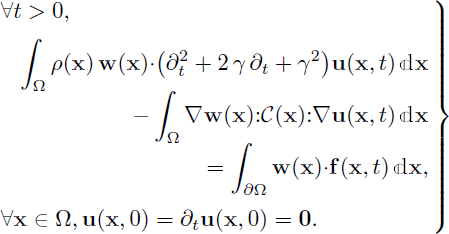8)

The solution u(x, t) of the forward problem (8) is called the forward field.

2.4 Misfit functional

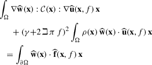
The displacement field is observed on the boundary ∂Ω (or on a portion of ∂Ω). From this measurement, denoted by u _obs(x, t), we want to image regions in Ω where the material properties differ from a known background material. For this purpose, the windowed measured field u _obs(x, t) is compared to its model prediction u _μ (x, t) for a given set μ = (ρ, 𝒞) by means of the following misfit functional involving the squares of windowed measurement residuals:

$$\begin{array}{cc}\hfill J(\mu )& =\frac{1}{2}{\int }_0^T{\int }_{\partial \mathrm{\Omega }}{[{\mathbf{u}}_{\mu }(\mathbf{x},t)-{\mathbf{u}}_{\mathrm{obs}}(\mathbf{x},t)]}^2\mathbb{d}\mathbf{x}\mathbb{d}t\hfill \\ \hfill & =\frac{1}{2}{\int }_0^T\left\{{\int }_{\partial \mathrm{\Omega }}{[{\underline{\mathbf{u}}}_{\mu }(\mathbf{x},t)-{\underline{\mathbf{u}}}_{\mathrm{obs}}(\mathbf{x},t)]}^2\mathbb{d}\mathbf{x}\right\}{\mathbb{e}}^{-2\gamma t}\mathbb{d}t.\hfill \end{array}$$(9)

The weighting applied to the observed physical signals decreases with time, in order to emphasize the first reflections over later multiple reflections. For this reason, we view our approach described next as using (9) for performing an Early-Reverberation Imaging (ERI).

A PDE-constrained (full-waveform) inversion approach would then consist in seeking a set μ that minimizes the (positive) misfit functional J(μ) subject to u _μ solving (8). In this work, we do not perform that minimization, but instead use J(μ) as a basis for defining imaging functions that provide information on μ. Let μ ₀ = (ρ ₀, 𝒞₀) denote the background (i.e. reference) value of μ corresponding to the healthy medium. Similarly to available topological imaging methods [13, 16, 17, 24], our approach exploits a linearization of J(μ) about μ ₀ and thus exploits only the first iteration of a complete iterative minimization process. Generally speaking, this linearization takes the form

$$\begin{array}{c}\hfill J({\mu }_0+\delta \mu )-J({\mu }_0)=\langle J^{\prime }({\mu }_0),\delta \mu \rangle +o(\Vert \delta \mu \Vert )\end{array}$$(10)

where J′(μ ₀) is the Fréchet derivative of J at the background medium.

In the present case, considering a small parameter variation δ μ(x) in the least-squares misfit functional (9), the first-order perturbation of J can be expressed as:

$$\begin{array}{cc}& J({\mu }_0+\delta \mu )-J({\mu }_0)\\ & ={\int }_0^T{\int }_{\mathrm{\partial }\mathrm{\Omega }}\delta \mathbf{u}(\mathbf{x},t)\cdot \mathbf{r}(\mathbf{x},t)\mathbb{d}\mathbf{x}\mathbb{d}t+o(\parallel \delta \mu \parallel ),\\ & \begin{array}{l}\\ & \text{with}& \delta \mathbf{u}(\mathbf{x},t)& ={\mathbf{u}}_{{\mu }_0+\delta \mu }(\mathbf{x},t)-{\mathbf{u}}_{{\mu }_0}(\mathbf{x},t)\\ & \text{and}& \mathbf{r}(\mathbf{x},t)& ={\mathbf{u}}_{{\mu }_0}(\mathbf{x},t)-{\mathbf{u}}_{\mathrm{o}\mathrm{b}\mathrm{s}}(\mathbf{x},t)\\ & \text{(measurement residual).}\end{array}\end{array}$$(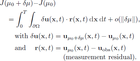11)

In (11) and hereafter, the perturbation of the windowed displacement field induced by δ μ is denoted by δ u(x, t) and the difference (called residual) between the calculated field and the observed field by r(x, t). The o(∥δ μ∥) remainder in (11) results from δ u being known from solution sensitivity analysis to have a O(∥δ μ∥) leading behaviour. The derivative J′(μ ₀) is then to be found from the O(∥δ μ∥) leading-order contribution to the integral term of (11). This task can be carried out by applying the well-known adjoint-state method to the present case, following the approach described in the survey article [6] (for least-squares migration applied to acoustic propagation in a fluid with unknown slowness to be mapped in space, both in frequency and time domains) or in [25] (for a weighted misfit functional and an elastic isotropic medium), among other references. In the present application-oriented context of using finite-element methods for solving partial differential equations, we prefer to derive J′(μ ₀) using weak formulations and basic linearization, rather than function-analytic methods.

2.5 Adjoint problem

We then define the adjoint problem as done in FWI or topological imaging methods, as follows: find v such that, for any test function w,

$$\begin{array}{c}\begin{array}{lr}\mathrm{\forall }t<T\text{,}& {\displaystyle {\int }_{\mathrm{\Omega }}\rho (\mathbf{x})\mathbf{w}(\mathbf{x})\cdot \left({\mathrm{\partial }}_t^2-2\gamma {\mathrm{\partial }}_t+{\gamma }^2\right)\mathbf{v}(\mathbf{x},t)\mathbb{d}\mathbf{x}}\\ & {\displaystyle +{\int }_{\mathrm{\Omega }}\mathrm{\nabla }\mathbf{w}(\mathbf{x}):\mathcal{C}(\mathbf{x}):\mathrm{\nabla }\mathbf{v}(\mathbf{x},t)\mathbb{d}\mathbf{x}}\\ & {\displaystyle ={\int }_{\mathrm{\partial }\mathrm{\Omega }}\mathbf{w}(\mathbf{x})\cdot \mathbf{r}(\mathbf{x},t)\mathbb{d}\mathbf{x}\text{,}}\\ \mathrm{\forall }\mathbf{x}\in \mathrm{\Omega }\text{,}& {\displaystyle \mathbf{v}(\mathbf{x},T)={\mathrm{\partial }}_t\mathbf{v}(\mathbf{x},T)=\mathbf{0}.}\end{array}\}\end{array}$$(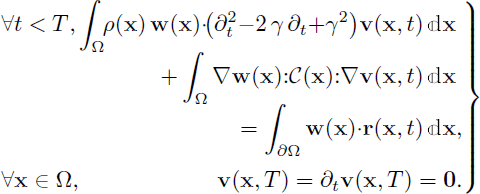12)

The solution v(x, t) of the adjoint problem (12), which includes final rest conditions, is called the adjoint field. Explicitly performing a time reversal t ↦ T − t in (12) recasts the adjoint problem in the same form as the forward problem (8), the original source term f(x, t) being replaced with the time-reversed measurement residual r(x, T − t). From the standpoint of physical units, r is a displacement (in m) whereas f is a surface force density (in N/m²), which will impact the definition of dimensionless imaging functions (Sect. 2.8).

2.6 Imaging functions

By rewriting equation (8) for both μ ₀ + δ μ and μ ₀, subtracting the resulting equalities and neglecting o(∥δ μ∥) higher-order contributions, we obtain the following identity, valid for any test function and at the first order in δ μ:

$$\begin{array}{cc}& {\int }_{\mathrm{\Omega }}\rho (\mathbf{x})\mathbf{w}(\mathbf{x})·({\partial }_t^2+2\gamma {\partial }_t+{\gamma }^2)\delta \mathbf{u}(\mathbf{x},t)\mathbb{d}\mathbf{x}\hfill \\ \hfill & +{\int }_{\mathrm{\Omega }}\mathrm{\nabla }\mathbf{w}(\mathbf{x}):\mathcal{C}(\mathbf{x}):\mathrm{\nabla }\delta \mathbf{u}(\mathbf{x},t)\mathbb{d}\mathbf{x}\hfill \\ \hfill & +{\int }_{\mathrm{\Omega }}\delta \rho (\mathbf{x})\mathbf{w}(\mathbf{x})·({\partial }_t^2+2\gamma {\partial }_t+{\gamma }^2)\mathbf{u}(\mathbf{x},t)\mathbb{d}\mathbf{x}\hfill \\ \hfill & +{\int }_{\mathrm{\Omega }}\mathrm{\nabla }\mathbf{w}(\mathbf{x}):\delta \mathcal{C}(\mathbf{x}):\mathrm{\nabla }\mathbf{u}(\mathbf{x},t)\mathbb{d}\mathbf{x}=0.\hfill \end{array}$$(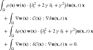13)

Then, replacing the test function w(x) by the adjoint field v(x, t) in (13) and by the forward field perturbation δ u(x, t) in (12), we obtain by difference:

$$\begin{array}{cc}\hfill {\int }_{\partial \mathrm{\Omega }}& \delta \mathbf{u}(\mathbf{x},t)·\mathbf{r}(\mathbf{x},t)\mathbb{d}\mathbf{x}\hfill \\ \hfill & ={\int }_{\mathrm{\Omega }}\rho (\mathbf{x})\delta \mathbf{u}(\mathbf{x},t)·({\partial }_t^2-2\gamma {\partial }_t)\mathbf{v}(\mathbf{x},t)\mathbb{d}\mathbf{x}\hfill \\ \hfill & -{\int }_{\mathrm{\Omega }}\rho (\mathbf{x})\mathbf{v}(\mathbf{x},t)·({\partial }_t^2+2\gamma {\partial }_t)\delta \mathbf{u}(\mathbf{x},t)\mathbb{d}\mathbf{x}\hfill \\ \hfill & -{\int }_{\mathrm{\Omega }}\delta \rho (\mathbf{x})\mathbf{v}(\mathbf{x},t)·({\partial }_t^2+2\gamma {\partial }_t+{\gamma }^2)\mathbf{u}(\mathbf{x},t)\mathbb{d}\mathbf{x}\hfill \\ \hfill & -{\int }_{\mathrm{\Omega }}\mathrm{\nabla }\mathbf{v}(\mathbf{x},t):\delta \mathcal{C}(\mathbf{x}):\mathrm{\nabla }\mathbf{u}(\mathbf{x},t)\mathbb{d}\mathbf{x},0\le t\le T.\hfill \end{array}$$(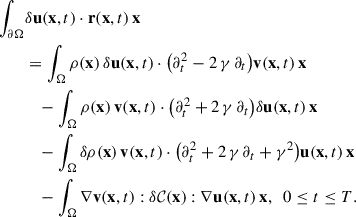14)

We next integrate (14) over t ∈ [0, T], using integration by parts in time together with the vanishing initial conditions on u and final conditions on v; this in particular causes the contributions of the first two terms of the right-hand side of (14) to cancel each other. Using the resulting value in (11) and recalling (10), we finally obtain

$$\begin{array}{cc}& \langle J^{\prime }({\mu }_0),\delta \mu \rangle \hfill \\ \hfill & =-{\int }_0^T{\int }_{\mathrm{\Omega }}\}\delta \rho (\mathbf{x})\mathbf{v}(\mathbf{x},t)·({\partial }_t^2+2\gamma {\partial }_t+{\gamma }^2)\mathbf{u}(\mathbf{x},t)\hfill \\ \hfill & +\mathrm{\nabla }\mathbf{v}(\mathbf{x},t):\delta \mathcal{C}(\mathbf{x}):\mathrm{\nabla }\mathbf{u}(\mathbf{x},t)\{\mathbb{d}\mathbf{x}\mathbb{d}t.\hfill \end{array}$$

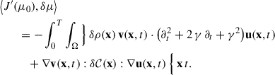
This result suggests to define imaging functions on the basis of the negative derivative of J at μ ₀, by setting

$$\begin{array}{cc}\hfill -\langle J^{\prime }({\mu }_0),\delta \mu \rangle & ={\int }_{\mathrm{\Omega }}{I}_{\rho }(\mathbf{x})\delta \rho (\mathbf{x})\mathbb{d}\mathbf{x}\hfill \\ \hfill & +\sum _{1\le \alpha \le \beta \le 6}{\int }_{\mathrm{\Omega }}{I}_{\alpha \beta }(\mathbf{x})\delta C_{\alpha \beta }(\mathbf{x})\mathbb{d}\mathbf{x}\hfill \end{array}$$

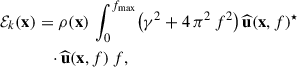
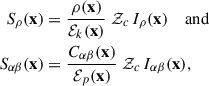
with the imaging function I _ρ for variations of the mass density ρ(x) given by

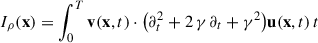$$\begin{array}{c}\hfill I_{\rho }(\mathbf{x})={\int }_0^T\mathbf{v}(\mathbf{x},t)·({\partial }_t^2+2\gamma {\partial }_t+{\gamma }^2)\mathbf{u}(\mathbf{x},t)\mathbb{d}t\end{array}$$(15)

and the imaging function I _{α β} for variations of the 21 stiffnesses C _{α β} (using Voigt indexing, 1 ≤ α ≤ β ≤ 6) given by

$$\begin{array}{cc}\hfill I_{\alpha \beta }(\mathbf{x})& =\frac{1}{1+{\delta }_{\alpha ,\beta }}{\int }_0^T\underset{\begin{array}{c}(i_1,j_1)\in \mathcal{E}(\alpha )\\ (i_2,j_2)\in \mathcal{E}(\beta )\end{array}}{[\sum }{\partial }_{i_1}{v}_{j_1}(\mathbf{x},t){\partial }_{i_2}{u}_{j_2}(\mathbf{x},t)\hfill \\ \hfill & +{\partial }_{i_2}{v}_{j_2}(\mathbf{x},t){\partial }_{i_1}{u}_{j_1}(\mathbf{x},t)]\mathbb{d}t,\hfill \end{array}$$(16)

where ℰ(α)={(α, α)} (α = 1, 2, 3), ℰ(4)={(2, 3),(3, 2)}, ℰ(5)={(1, 3),(3, 1)} and ℰ(6)={(1, 2),(2, 1)} and δ is the Kronecker symbol. Each imaging function thus defined is hence positive when the estimate of the real value of the corresponding parameter found by solving for δ μ the linearized equation J(μ ₀ + δ μ)=J(μ ₀)+⟨J′(μ ₀),δ μ⟩ is greater than the value μ ₀ for the healthy medium.

The imaging functions (15) and (16) are defined on the basis of the Fréchet derivative (10), where the smallness of perturbations δ μ is measured in terms of the supremum norm ∥δ μ∥=∥δ μ∥_∞ := sup _x ∈ Ω|δ μ(x)|. Imaging functions may alternatively be formulated from the topological derivative of J [12, 13], whose definition rests on the smallness of δ μ being measured in terms of the volume of its geometrical support (finite material variations being allowed in that case). The mass density imaging functions arising from both approaches are the same, while the stiffness imaging functions take distinct forms (both bilinear in u, v).

2.7 Rewriting the equations in the frequency domain

All the fields are of practically finite duration T. Moreover, their frequencies are assumed to be less than a maximum f _max, such that the direct and inverse Fourier transforms defined by

$$\begin{array}{c}\begin{array}{c}\underbrace{{\displaystyle \hat{\mathbf{w}}(\mathbf{x},f)={\int }_0^T\mathbf{w}(\mathbf{x},t)\exp (-2\mathbb{i}\pi ft)\mathbb{d}t}}\\ \Updownarrow \\ \overbrace{{\displaystyle \mathbf{w}(\mathbf{x},t)={\int }_{-f_{max}}^{f_{max}}\hat{\mathbf{w}}(\mathbf{x},f)\exp (2\mathbb{i}\pi ft)\mathbb{d}t,}}\end{array}\end{array}$$

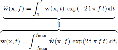
can be calculated numerically by fast Fourier transform.

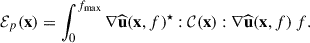
By virtue of Parseval’s equality and the real-valuedness of u, v, the imaging functions can also be written as follows. From equation (15), an alternative expression of the mass density imaging function is

$$\begin{array}{c}\hfill I_{\rho }(\mathbf{x})=2\mathfrak{R}[{\int }_0^{f_{max}}{(\gamma +2\mathbb{i}\pi f)}^2\widehat{\mathbf{v}}{(\mathbf{x},f)}^{\star }·\widehat{\mathbf{u}}(\mathbf{x},f)\mathbb{d}f]\end{array}$$(17)

while the stiffness imaging functions (16) take the form

$$\begin{array}{cc}\hfill I_{\alpha \beta }(\mathbf{x})& =\frac{2}{1+{\delta }_{\alpha ,\beta }}\mathfrak{R}\{{\int }_0^{f_{max}}\underset{\begin{array}{c}(i_1,j_1)\in \mathcal{E}(\alpha )\\ (i_2,j_2)\in \mathcal{E}(\beta )\end{array}}{[\sum }\hfill \\ & {\partial }_{i_1}{\widehat{v}}_{j_1}{(\mathbf{x},f)}^{\star }{\partial }_{i_2}{\widehat{u}}_{j_2}(\mathbf{x},f)\hfill \\ & +{\partial }_{i_2}{\widehat{v}}_{j_2}{(\mathbf{x},f)}^{\star }{\partial }_{i_1}{\widehat{u}}_{j_1}(\mathbf{x},f)]\mathbb{d}f\}.\hfill \end{array}$$(18)

Expressions (17), (18) will be computed by summation over a finite set ℱ ⊂ [0, f _max] of discrete frequencies, with a sampling step just under 1/T. The Fourier transforms $\widehat{\mathbf{u}}(\mathbf{x},f)$ and $\widehat{\mathbf{v}}{(\mathbf{x},f)}^{\star }$ of the forward field and of the conjugated adjoint field, respectively, are directly computed in the frequency domain for f ∈ ℱ.

Writing the wave equation (6) in the frequency domain and recasting it in weak form by usual methods, the forward field $\widehat{\mathbf{u}}$ is found to satisfy from equation (8):

$$\begin{array}{cc}& {\int }_{\mathrm{\Omega }}\mathrm{\nabla }\widehat{\mathbf{w}}(\mathbf{x}):\mathcal{C}(\mathbf{x}):\mathrm{\nabla }\widehat{\mathbf{u}}(\mathbf{x},f)\mathbb{d}\mathbf{x}\hfill \\ \hfill & {+(\gamma +2\mathbb{i}\pi f)}^2{\int }_{\mathrm{\Omega }}\rho (\mathbf{x})\widehat{\mathbf{w}}(\mathbf{x})·\widehat{\mathbf{u}}(\mathbf{x},f)\mathbb{d}\mathbf{x}\hfill \\ \hfill & ={\int }_{\partial \mathrm{\Omega }}\widehat{\mathbf{w}}(\mathbf{x})·\widehat{\mathbf{f}}(\mathbf{x},f)\mathbb{d}\mathbf{x}\hfill \end{array}$$

for any test function $\widehat{\mathbf{w}}$. Similarly, the conjugated adjoint field ${\widehat{\mathbf{v}}}^{\star }$ satisfies, for any test function $\widehat{\mathbf{w}}$, the same equation with a different source term:

$$\begin{array}{cc}& {\int }_{\mathrm{\Omega }}\mathrm{\nabla }\widehat{\mathbf{w}}(\mathbf{x}):\mathcal{C}(\mathbf{x}):\mathrm{\nabla }\widehat{\mathbf{v}}{(\mathbf{x},f)}^{\star }\mathbb{d}\mathbf{x}\hfill \\ \hfill & {+(\gamma +2\mathbb{i}\pi f)}^2{\int }_{\mathrm{\Omega }}\rho (\mathbf{x})\widehat{\mathbf{w}}(\mathbf{x})·\widehat{\mathbf{v}}{(\mathbf{x},f)}^{\star }\mathbb{d}\mathbf{x}\hfill \\ \hfill & ={\int }_{\partial \mathrm{\Omega }}\widehat{\mathbf{w}}(\mathbf{x})·\widehat{\mathbf{r}}{(\mathbf{x},f)}^{\star }\mathbb{d}\mathbf{x}.\hfill \end{array}$$

The conjugation of $\widehat{\mathbf{v}}$ and $\widehat{\mathbf{r}}$ of course reflects the time reversal inherent in the definition of the adjoint field.

In practice, a single problem generally with different canonical source terms is solved with a finite element code for the set ℱ of frequencies, as detailed below. The different solutions are then stored in memory. Finally, the discrete Fourier transforms of the windowed sampled excitation and residual are successively taken as input to obtain the forward and adjoint fields.

2.8 Normalization of the imaging functions

Not all areas of the domain Ω are insonified in the same way. The total energy density per unit volume received at position x is the sum of the volume densities e _k (x) and e _p (x) of kinetic and strain energies of the direct field, respectively. Their summation over time leads to the cumulative kinetic energy density

$$\begin{array}{c}\hfill {\mathcal{E}}_k(\mathbf{x})=\rho (\mathbf{x}){\int }_0^{f_{max}}({\gamma }^2+4{\pi }^2{f}^2)\widehat{\mathbf{u}}{(\mathbf{x},f)}^{\star }·\widehat{\mathbf{u}}(\mathbf{x},f)\mathbb{d}f,\end{array}$$(19)

and the cumulative strain energy density

$$\begin{array}{c}\hfill {\mathcal{E}}_p(\mathbf{x})={\int }_0^{f_{max}}\mathrm{\nabla }\widehat{\mathbf{u}}{(\mathbf{x},f)}^{\star }:\mathcal{C}(\mathbf{x}):\mathrm{\nabla }\widehat{\mathbf{u}}(\mathbf{x},f)\mathbb{d}f.\end{array}$$(20)

Therefore, dimensionless imaging functions S _ρ and S _{α β} can be defined from the imaging functions I _ρ and I _{α β} as

$$\begin{array}{cc}\hfill S_{\rho }(\mathbf{x})& =\frac{\rho (\mathbf{x})}{{\mathcal{E}}_k(\mathbf{x})}{\mathcal{Z}}_c{I}_{\rho }(\mathbf{x})\text{and}\hfill \\ \hfill S_{\alpha \beta }(\mathbf{x})& =\frac{C_{\alpha \beta }(\mathbf{x})}{{\mathcal{E}}_p(\mathbf{x})}{\mathcal{Z}}_c{I}_{\alpha \beta }(\mathbf{x}),\hfill \end{array}$$(21)

where 𝒵 _c is a scaling factor corresponding to the modulus of a characteristic impedance (ratio of surface force over displacement, in N/m³) on the receivers area. This scaling factor compensates for the physical unit mismatch between the adjoint loading r and the applied excitation f, see Section 2.5 above. It is arbitrarily defined using characteristic quantities of the problem at hand (see Sect. 3.3), and this results in the dimensionless imaging functions taking values of the order of unity. In addition to easing interpretation, the use of cumulative energy densities ℰ _k (x) and ℰ _p (x) to correct the imaging functions in definition (21) serves to enhance the imaging potential in areas where the insonification results in comparatively low energy levels, for instance due to not being in direct line of sight from the transducers.

3 A 2D numerical test case

3.1 Medium geometry and transducer location

The medium under investigation is denoted as Ω_obs, and it is assumed to be composed of an orthotropic material. The anomalies tested in the study are described in Section 3.4. Outside the region of the anomaly to be imaged, the medium is assumed to be aluminum. Therefore, the reference medium Ω is considered homogeneous and made of aluminum. Thus the corresponding measurements can be exploited only if providing information gleaned by way of multiple reflections on the boundaries of the propagation domain. The geometry, material parameters and excitation signals for the test case are assumed to be translationally invariant along the x ₃ coordinate, so that all relevant field quantities only depend on the coordinates x ₁, x ₂ of points in the 2D cross-section Ω, shown in Figure 1.

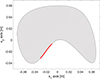Figure 1. Reference medium Ω of the test case. The thick line is part of ∂Ω and indicates the transducer surface that is split into eight independent transducers used both for emission and reception.

Eight transducers, each 4 mm long, are simulated and cover the thick line on the edge of the domain drawn in Figure 1. Under the 2D assumption, wave propagation is confined to the (x ₁ , x ₂ )-plane and can exhibit two types of polarization: in-plane polarization (including longitudinal and in-plane transverse waves) and out-of-plane polarization (transverse waves polarized in the x ₃ -direction). For simulations involving in-plane polarization, waves are generated using a stress vector f oriented normal to ∂Ω and lying within the (x ₁ , x ₂ )-plane. For out-of-plane polarization simulations, the stress vector f is oriented along the x ₃ -axis.

The excitation signal is a 3-cycle Gaussian-windowed sine burst of central frequency 300 kHz. The corresponding wavelengths for the background medium and at this central frequency are 10 and 21 mm for transverse and longitudinal waves, respectively. The transducers are thus smaller than half of the smallest wavelength. Displacement measurements are simulated by computing the integral of the displacement vector over the surface area of each transducer.

3.2 Wave equations and finite element modelling

Due to the assumed translational invariance, the frequency-domain version of the wave equation (6) reduces to two uncoupled 2D wave equations. Firstly, the in-plane components ${\widehat{u}}_1,{\widehat{u}}_2$ of $\widehat{\mathbf{u}}$, corresponding to the propagation of both compressional and shear waves carrying a polarization in the (x ₁, x ₂) plane, satisfy

$$\begin{array}{cc}& \rho {(\gamma +2\mathbb{i}\pi f)}^2\left(\begin{array}{c}{\widehat{u}}_1\\ [1mm]{\widehat{u}}_2\end{array}\right)\hfill \\ \hfill & -\left\{\begin{array}{c}{\partial }_1(C_{11}{\partial }_1{\widehat{u}}_1+C_{12}{\partial }_2{\widehat{u}}_2)+{\partial }_2\left[C_{66}({\partial }_1{\widehat{u}}_2+{\partial }_2{\widehat{u}}_1)\right]\\ [1mm]{\partial }_1\left[C_{66}({\partial }_1{\widehat{u}}_2+{\partial }_2{\widehat{u}}_1)\right]+{\partial }_2(C_{12}{\partial }_1{\widehat{u}}_1+C_{22}{\partial }_2{\widehat{u}}_2)\end{array}\right\}\hfill \\ \hfill & =\left(\begin{array}{c}0\\ [1mm]0\end{array}\right).\hfill \end{array}$$(22)

This will be referred as the in-plane polarization case in what follows. Secondly, the out-of-plane component ${\widehat{u}}_3$, corresponding to the propagation of shear waves with out-of-plane polarization along the x ₃-direction, satisfies

$$\begin{array}{cc}& \rho (\gamma +2\mathbb{i}\pi f{)}^2{\hat{u}}_3-[{\mathrm{\partial }}_1\left(C_{55}{\mathrm{\partial }}_1{\hat{u}}_3\right)+{\mathrm{\partial }}_2\left(C_{44}{\mathrm{\partial }}_2{\hat{u}}_3\right)]=0.\end{array}$$(23)

Equations (22) and (23) are recast in the appendix in a form allowing their implementation in Comsol [26]. They are used at two stages. First, synthetic values of the experimental data u _obs are computed by solving them with material parameters set to the perturbed values to be imaged and on a mesh that explicitly models the anomaly. Then, the forward and adjoint fields entering the imaging functions are solved in the form (22) and (23) with the background material parameters and on a distinct imaging mesh that is not affected by the anomaly geometry.

It has to be emphasized that the translational invariance along x ₃ is also assumed for the sources and the receivers. In practical applications with bounded transducers, this hypothesis is valid if the transducer dimension along the x ₃-axis is large enough relative to the wavelength.

3.3 Imaging functions for the 2D case

3.3.1 A single scaling factor common to both polarization cases

The scaling factor 𝒵 _c for the dimensionless imaging functions is set to 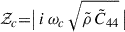${\mathcal{Z}}_c=|\mathbb{i}{\omega }_c\sqrt{\tilde{\rho }{\tilde{C}}_{44}}|$. This value, suitable for both the in-plane and out-of-plane cases discussed below, uses the mass density $\tilde{\rho }$ and the stiffness ${\tilde{C}}_{44}$ of the material near the receivers, and the central angular frequency ω _c of the excitation signal.

3.3.2 The in-plane polarization case

For the in-plane polarization case, the mass density imaging function I _ρ (x) given by equation (17) becomes

$$\begin{array}{cc}\hfill I_{\rho }(\mathbf{x})& ={2\mathfrak{R}[{\int }_0^{f_{max}}(\gamma +2\mathbb{i}\pi f)}^2({\widehat{v}}_1{(\mathbf{x},f)}^{\star }{\widehat{u}}_1(\mathbf{x},f)\hfill \\ \hfill & +{\widehat{v}}_2{(\mathbf{x},f)}^{\star }{\widehat{u}}_2(\mathbf{x},f))\mathbb{d}f],\hfill \end{array}$$

while the stiffness imaging functions I _{α β} given by equation (18) become

$$\begin{array}{cc}\hfill I_{11}(\mathbf{x})& =2\mathfrak{R}\left[{\int }_0^{f_{max}}{\partial }_1{\widehat{v}}_1{(\mathbf{x},f)}^{\star }{\partial }_1{\widehat{u}}_1(\mathbf{x},f)\mathbb{d}f\right],\hfill \\ \hfill I_{22}(\mathbf{x})& =2\mathfrak{R}\left[{\int }_0^{f_{max}}{\partial }_2{\widehat{v}}_2{(\mathbf{x},f)}^{\star }{\partial }_2{\widehat{u}}_2(\mathbf{x},f)\mathbb{d}f\right],\hfill \\ \hfill I_{12}(\mathbf{x})& =2\mathfrak{R}[{\int }_0^{f_{max}}{\partial }_1{\widehat{v}}_1{(\mathbf{x},f)}^{\star }{\partial }_2{\widehat{u}}_2(\mathbf{x},f)\hfill \\ \hfill & +{\partial }_2{\widehat{v}}_2{(\mathbf{x},f)}^{\star }{\partial }_1{\widehat{u}}_1(\mathbf{x},f)\mathbb{d}f],\hfill \\ \hfill I_{66}(\mathbf{x})& ={2\mathfrak{R}\{{\int }_0^{f_{max}}[{\partial }_1{\widehat{v}}_2(\mathbf{x},f)+{\partial }_2{\widehat{v}}_1(\mathbf{x},f)]}^{\star }\hfill \\ \hfill & [{\partial }_1{\widehat{u}}_2(\mathbf{x},f)+{\partial }_2{\widehat{u}}_1(\mathbf{x},f)]\mathbb{d}f\}.\hfill \end{array}$$

The formulas (19) and (20) giving the cumulative kinetic and strain energy densities take the more-explicit form

$$\begin{array}{cc}\hfill {\mathcal{E}}_k(\mathbf{x})& =\rho (\mathbf{x}){\int }_0^{f_{max}}({\gamma }^2+4{\pi }^2{f}^2)\hfill \\ \hfill & (|{\widehat{u}}_1{(\mathbf{x},f)|}^2+{|{\widehat{u}}_2(\mathbf{x},f)|}^2)\mathbb{d}f\hfill \end{array}$$

and

$$\begin{array}{cc}\hfill {\mathcal{E}}_p(\mathbf{x})& ={\int }_0^{f_{max}}\{C_{11}{(\mathbf{x})\left|{\widehat{\mathrm{\epsilon }}}_{11}(\mathbf{x},f)\right|}^2\hfill \\ \hfill & +C_{22}(\mathbf{x}){{\left|{\widehat{\mathrm{\epsilon }}}_{22}(\mathbf{x},f)\right|}^2+4C_{66}(\mathbf{x})\left|{\widehat{\mathrm{\epsilon }}}_{12}(\mathbf{x},f)\right|}^2\hfill \\ \hfill & +2C_{12}(\mathbf{x})\mathfrak{R}[{\widehat{\mathrm{\epsilon }}}_{11}^{\star }(\mathbf{x},f){\widehat{\mathrm{\epsilon }}}_{22}(\mathbf{x},f)]\}\mathbb{d}f,\hfill \end{array}$$

where ${\widehat{\mathrm{\epsilon }}}_{\mathit{ij}}(\mathbf{x},f)=({\partial }_i{u}_j(\mathbf{x},f)+{\partial }_j{u}_i(\mathbf{x},f))/2$ denotes the i j-component of the linearized strain tensor associated to the displacement field $\widehat{\mathbf{u}}$.

3.3.3 The out-of-plane polarization case

For the out-of-plane polarization case, the density imaging function I _ρ (x) given by equation (17) becomes

$$\begin{array}{c}\hfill I_{\rho }(\mathbf{x})=2\mathfrak{R}\left[{\int }_0^{f_{max}}{(\gamma +2\mathbb{i}\pi f)}^2{\widehat{v}}_3{(\mathbf{x},f)}^{\star }{\widehat{u}}_3(\mathbf{x},f)\mathbb{d}f\right],\end{array}$$

the stiffness imaging functions I _{α β} given by equation (18) are rewritten as

$$\begin{array}{cc}\hfill I_{44}(\mathbf{x})& =2\mathfrak{R}\left[{\int }_0^{f_{max}}{\partial }_2{\widehat{v}}_3{(\mathbf{x},f)}^{\star }{\partial }_2{\widehat{u}}_3(\mathbf{x},f)\mathbb{d}f\right],\hfill \\ \hfill I_{55}(\mathbf{x})& =2\mathfrak{R}\left[{\int }_0^{f_{max}}{\partial }_1{\widehat{v}}_3{(\mathbf{x},f)}^{\star }{\partial }_1{\widehat{u}}_3(\mathbf{x},f)\mathbb{d}f\right],\hfill \end{array}$$

and formulas (19) and (20) giving the cumulative kinetic and strain energy densities become:

$$\begin{array}{cc}\hfill {\mathcal{E}}_k(\mathbf{x})& =\rho (\mathbf{x}){\int }_0^{f_{max}}({\gamma }^2+4{\pi }^2{f}^2)|{\widehat{u}}_3{(\mathbf{x},f)|}^2\mathbb{d}f\hfill \\ \hfill {\mathcal{E}}_p(\mathbf{x})& =4{\int }_0^{f_{max}}[C_{44}{(\mathbf{x})\left|{\widehat{\mathrm{\epsilon }}}_{23}(\mathbf{x},f)\right|}^2\hfill \\ \hfill & +C_{55}{(\mathbf{x})\left|{\widehat{\mathrm{\epsilon }}}_{13}(\mathbf{x},f)\right|}^2]\mathbb{d}f.\hfill \end{array}$$

3.4 Results

The medium anomaly to be imaged for this example is a circular inclusion D of diameter 2 mm, located in an area masked from the transducer array and supporting a material perturbation such that either ρ = 0.5 ρ ₀ or C ₁₁ = 0.5 (𝒞₀)₁₁. The material properties outside of D are those of the homogeneous background medium. The transducers are located according to the description of Figure 1. It has to be emphasized that in such a configuration, there is no direct path for the waves propagating between the transducers and the perturbation. Thus the images only rely on waves reflected multiple times on the domain boundaries. As no dissipation is modelled, the theoretical elastodynamic field does not decay with time. Recall that the proposed imaging method relies on an exponentially decaying time-domain truncation window, which can also be interpreted as a weighting window used in the misfit functional (9).

The images of the test case shown below were obtained by averaging eight images, each acquired with a different transducer acting as the sole emitter. This acquisition procedure is also known as the full matrix capture [1].

3.4.1 Practical design of the decaying window

The decaying window t ↦ exp(−γ t) is designed to satisfy two requirements, namely, (i) the window duration T is larger than the first back and forth propagation duration t _BF from the emitter to the receiver through the region of interest, and (ii) the “tail” of the windowed fields for t >  T is of sufficiently small magnitude. This design rests on the values of T and γ. Under the present conditions, we have t _BF ≈ 100 μs (an exact value can hardly be given as there are an infinity of propagation paths with potential polarization conversion, due to Ω being bounded). Thus requirement (i) is here fulfilled choosing T  ≥  100 μs. Requirement (ii) is met by setting exp(−γ T)  =  10^−m for some m >  0 and we chose m  =  3. In order to give some insight on the effect of the value of T, different values are tested for the masked density perturbation and the resulting density images are presented in Figure 2. In the interest of conciseness, the results are presented for the in-plane wave case only.

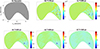Figure 2. (a) Geometry of the investigated domain. The localized density perturbation is contained in the circle where the density is twice smaller than in the surrounding region. (b)–(f) Density images I ρ obtained using different decaying window duration and in-plane waves.

A T  =  100 μs duration is too short, as artifacts are dominant (Fig. 2b). All larger values (c–f) used give satisfactory results as the region of lower density is accurately located and the negative extremum does indicate a region of smaller mass density. The localized artifacts on the right of the perturbation (b–d) tend to decrease, while the overall background noise tends to increase, as T is increased. At this stage we do not have an automatic method for finding the best value of the duration T, which depends on the medium shape, on the presence or absence of direct wave path, on the size of the perturbation and on its contrast to the surrounding environment. The choice of T also determines the frequency step Δf = 1/T used in the computations, and thus drives the computation cost. In the present example, an empirical compromise is chosen by setting T  =  800 μs for both cases studied hereafter.

3.4.2 Locating a masked density variation

The local density variation to be imaged can be seen in the density map of Figure 3a. All the different gradients and energies are computed and the dimensionless imaging functions S _ρ and S _{α β} are shown in Figures 3b–3d for out-of-plane polarization and in Figures 3e–3i for in-plane polarization. Following the qualitative observations of the former section, the same window duration T  =  800 μs is chosen for all imaging functions.

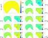Figure 3. The density distribution of the test case (a) and the normalized imaging functions obtained in the reference medium with out-of-plane polarization (b–d) and in-plane polarization (e–i).

For both polarizations, S _ρ presents a local minimum at the location of the real inhomogeneity, which indicates an accurate location of the perturbation while its negative sign correctly predicts a mass density value smaller than the background value. However all other S _{α β} functions are nonzero near the inhomogeneity location. This could be expected, as the underlying inverse problem is ill-posed: two different parameter sets may produce the same acoustic signature at the transducer location. For instance, it is likely that introducing two C ₁₁ inhomogeneities with higher values on both sides of the actual inhomogeneity location leads to a similar signature (Fig. 3f). Still, it is remarkable that the imaging functions S _{α β} exhibit a specific pattern linked with the axis direction corresponding to α and β. For instance S ₂₂ has an influence on the longitudinal waves propagating along the x ₂-direction and S ₄₄ on the out-of-plane transverse waves also propagating along the x ₂-direction. They both exhibit two spots surrounding the real inhomogeneity in the x ₂-direction.

In the present case and under the supplementary assumption of an unknown but single localized inhomogeneity, the comparison of those functions would allow the identification of a density inhomogeneity.

3.4.3 Locating a masked C₁₁ variation

The actual local C ₁₁ variation can be seen in the C ₁₁ map presented in Figure 4a. All the requisite gradients and energies are computed, to obtain the imaging functions S _ρ and S _{α β} presented in Figures 4b–4d for out-of-plane polarization and in Figures 4e–4i for in-plane polarization.

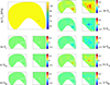Figure 4. The C 11 distribution of the test case (a) and the normalized imaging functions obtained in the reference medium with out-of-plane polarization (b–d) and in-plane polarization (e–i).

The imaging function S ₁₁ presents a local minimum at the location of the real inhomogeneity, which indicates an accurate location of the perturbation, and its negative sign correctly predicts a stiffness value that is smaller than the background value. As C ₁₁ has influence only on the longitudinal waves, the functions S ₄₄, S ₅₅ and S ₆₆ that only affect transverse waves take negligible values. However an ambiguity clearly occurs when trying to identify the nature of the inhomogeneity, since S ₁₁, S ₂₂ and S ₁₂ exhibit a similar behavior. The supplementary assumption of an unknown but single localized inhomogeneity would only eliminate the possibility of a mass density inhomogeneity.

3.4.4 Discussion on the robustness versus geometry accuracy

In both cases presented in Figures 3 and 4, the boundaries of the investigated perturbed medium and of the reference medium (used for computing forward and adjoint fields) are exactly identical. In practical, the geometry of the boundaries of the experimental medium is described with a limited accuracy. This may lead to inaccurate interpretation of the measured signals especially if many multiple reflection are taken into account. Thus the longer the decaying window is, the more sensitive to inaccuracy is expected to be the image processing. This is exactly the interest of controlling the decaying window. It is meant to offer the possibility of finding a compromise for exploiting the rich acoustic information of multiply reflected waves in a realistic environment. A systematic study of the optimization of the duration T with respect to the uncertainties on both the domain shape and mechanical parameters of the healthy medium is out of the scope of this paper. A simple example is presented in Figure 5 to give a first clue on that matter. The reference medium is the same as before but the shape of the investigated perturbed medium exhibits respectively a slight discrepancy at the right bottom (Fig. 5a) and a larger one (Fig. 5d). The images obtained with window durations of T = 200 μs and T = 800 μs are presented. The respective discrepancies are 2 and 5 mm corresponding to 0.2 λ₀ and 0.5 λ₀ where λ₀ corresponds to the wavelength of transverse waves at the central frequency.

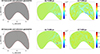Figure 5. (a) & (d) Geometries of the investigated and reference (red boundary) domains. The localized density perturbation is contained in the circle where the density is twice smaller than in the surrounding region. (b) & (c) Density images I ρ obtained using different decaying window duration and in-plane waves for the medium presented in (a). (e)–(f) Density images I ρ obtained using different decaying window duration and in-plane waves for the medium presented in (d).

Figure 6. Images S ρ obtained for a local density anomaly in front of the transducer array, using in-plane waves and different decaying window durations.

In both cases, the perturbation is better located and identified using a shorter duration (T = 200 μs) than that chosen when the medium geometry was assumed to be perfectly known (T = 800 μs). In the case where the geometry discrepancy is small (Fig. 5a), the perturbation is accurately identified as a smaller density for both window duration (Figs. 5b and 5c) but the artifacts are stronger with the longer window. In the case where the geometry discrepancy is larger (Fig. 5d), a second extremum appears near the perturbation location with a positive sign. Taking T = 200 μs (Fig. 5e), it is of similar magnitude as the awaited minimum. With the longest window, the maximum exceeds the minimum in magnitude. Beside larger artifacts, the other consequence of the too long window is a misidentification of the perturbation as being a higher density region. These results demonstrate that the truncation window is also a tool for mitigating the effects of an inaccurate knowledge of the medium geometry or material properties and still takes advantage of multiply reflected acoustic information.

3.4.5 Performance of ERI for a defect in direct view from the transducers

While the ERI method allows to localize defects that are not in direct view from the transducers, it is useful to also examine its performance for a defect in direct view. Numerical experiments are performed in the same reference medium, with a local density anomaly inserted this time in front of the transducer array. Corresponding images are presented in Figure 6 for different window durations.

The image obtained with a short window duration (Fig. 6a) is similar to that expected with a classical delay and sum method before applying a spatial envelope. This can be explained by the fact that with such a short duration, multiply reflected waves are neglected, which amounts to assuming a semi-infinite homogeneous domain such as that implied in delay and sum methods. When increasing the window duration (Figs. 6b and 6c), the signature of the defect in the image is getting more similar to its actual shape. Increasing window durations also leads to increasing pixel intensity in the defect vicinity. These two observations combined show that the wave interferences operating in the imaging function for longer window durations both reduce artifacts and increase the coherent reconstruction of the investigated domain. Thus, the ERI method also takes advantage of the reverberated data when imaging defects in direct view from the transducers.

4 Conclusion

The foundations of the early-reverberation imaging (ERI) method are now established. RI is motivated by the quest for a realistic compromise between the rich information contained in reverberated measurements and imaging robustness. In this paper, a mathematical framework is proposed and illustrated with a numerical two-dimensional test case. Distinct ERI functions have been defined in order to specifically image anomalies in either the mass density or one of the elastic stiffnesses. The proposed ERI method is particularly convenient for imaging elastic confined media where the inspected area is not directly visible from the ultrasonic transducers, as demonstrated in the presented test case. The many possibilities opened by the proposed approach will be explored in follow-up work. In particular, comprehensive investigations still need to be conducted on (i) the influence of the duration T and the γ parameter on the imaging performance and robustness and (ii) the sensivity of the imaging functions to uncertainties on the geometry.

Funding

The authors received no funding to complete this research.

Conflicts of interest

The authors declare no conflict of interest.

Data availability statement

No new data were created or analysed in this study.

References

Appendix A

PDE formulation for Comsol software

Using the Comsol partial differential equation module formalism [26], a complex angular frequency is defined:

$$\begin{array}{c}\hfill \omega =2\pi f-\gamma \mathbb{i}\end{array}$$

and equations (22) and (23) are implemented as follows:

$$\begin{array}{cc}\rho {\omega }^2\left(\begin{array}{c}{\hat{u}}_1\\ {\hat{u}}_2\end{array}\right)& +\mathrm{\nabla }\cdot \left\{\left[\begin{array}{cc}\left(\begin{array}{cc}{C}_{11}& 0\\ 0& C_{66}\end{array}\right)& \left(\begin{array}{cc}0& C_{12}\\ C_{66}& 0\end{array}\right)\\ \left(\begin{array}{cc}0& C_{66}\\ C_{12}& 0\end{array}\right)& \left(\begin{array}{cc}{C}_{66}& 0\\ 0& C_{22}\end{array}\right)\end{array}\right]\mathrm{\nabla }\left(\begin{array}{c}{\hat{u}}_1\\ {\hat{u}}_2\end{array}\right)\right\}\\ & =\left(\begin{array}{c}0\\ 0\end{array}\right)\\ \text{and}\rho {\omega }^2{\hat{u}}_3& +\mathrm{\nabla }\cdot \left(\begin{array}{cc}{C}_{55}& 0\\ 0& C_{44}\end{array}\right)\mathrm{\nabla }{\hat{u}}_3=0.\end{array}$$

All Figures

	Figure 1. Reference medium Ω of the test case. The thick line is part of ∂Ω and indicates the transducer surface that is split into eight independent transducers used both for emission and reception.
In the text

	Figure 2. (a) Geometry of the investigated domain. The localized density perturbation is contained in the circle where the density is twice smaller than in the surrounding region. (b)–(f) Density images I ρ obtained using different decaying window duration and in-plane waves.
In the text

	Figure 3. The density distribution of the test case (a) and the normalized imaging functions obtained in the reference medium with out-of-plane polarization (b–d) and in-plane polarization (e–i).
In the text

	Figure 4. The C 11 distribution of the test case (a) and the normalized imaging functions obtained in the reference medium with out-of-plane polarization (b–d) and in-plane polarization (e–i).
In the text

Figure 5. (a) & (d) Geometries of the investigated and reference (red boundary) domains. The localized density perturbation is contained in the circle where the density is twice smaller than in the surrounding region. (b) & (c) Density images I ρ obtained using different decaying window duration and in-plane waves for the medium presented in (a). (e)–(f) Density images I ρ obtained using different decaying window duration and in-plane waves for the medium presented in (d).

In the text

	Figure 6. Images S ρ obtained for a local density anomaly in front of the transducer array, using in-plane waves and different decaying window durations.
In the text

References

- C. Holmes, B.W. Drinkwater, P.D. Wilcox: Post-processing of the full matrix of ultrasonic transmit-receive array data for non-destructive evaluation. NDT & e International 38, 8 (2005) 701–711. [Google Scholar]
- J.F. Claerbout: Toward a unified theory of reflector mapping. Geophysics 36, 3 (1971) 467–481. [Google Scholar]
- P. Lailly: The seismic inverse problem as a sequence of before stack migrations, in: Proc. Conf. on Inverse Scattering, Theory and Applications. SIAM, Philadelphia, 1983, pp. 206–220. [Google Scholar]
- A. Tarantola: Inversion of seismic reflection data in the acoustic approximation. Geophysics 49, 8 (1984) 1259–1266. [CrossRef] [Google Scholar]
- A. Ernoult, J. Chabassier, S. Rodriguez, A. Humeau: Full waveform inversion for bore reconstruction of woodwind-like instruments. Acta Acustica 5 (2021) 47. [CrossRef] [EDP Sciences] [Google Scholar]
- R.-E. Plessix: A review of the adjoint-state method for computing the gradient of a functional with geophysical applications. Geophysical Journal International 167, 2 (2006) 495–503. [CrossRef] [Google Scholar]
- G. Chavent: Identification of distributed parameter systems: about the output least square method, its implementation, and identifiability. IFAC Proceedings Volumes 12, 8 (1979) 85–97. [Google Scholar]
- J. Virieux, S. Operto: An overview of full-waveform inversion in exploration geophysics. Geophysics 74, 6 (2009) WCC1–WCC26. [CrossRef] [Google Scholar]
- J. Tromp: Seismic wavefield imaging of Earth’s interior across scales. Nature Reviews Earth & Environment 1 (2020) 40–53. [Google Scholar]
- M. Bonnet, W. Aquino: Three-dimensional transient elastodynamic inversion using an error in constitutive relation functional. Inverse Problems 31, 3 (2015) 035010. [Google Scholar]
- S. Ghosh, Z. Zou, O. Babaniyi, W. Aquino, M.I. Diaz, M. Bayat, M. Fatemi: Modified error in constitutive equations (MECE) approach for ultrasound elastography. Journal of the Acoustical Society of America 142, 4 (2017) 2084–2093. [Google Scholar]
- H. Eschenauer, V. Kobelev, A. Schumacher: Bubble method for topology and shape optimization of structures. Structural Optimization 8 (1984) 42–51. [Google Scholar]
- M. Bonnet, B.B. Guzina: Sounding of finite solid bodies by way of topological derivative. International Journal for Numerical Methods in Engineering 61, 13 (2004) 2344–2373. [Google Scholar]
- B.B. Guzina, A.I. Madyarov: A linear sampling approach to inverse elastic scattering in piecewise-homogeneous domains. Inverse Problems 23, 4 (2007) 1467. [Google Scholar]
- M. Fink: Time reversal of ultrasonic fields. I. Basic principles. IEEE Transactions on Ultrasonics, Ferroelectrics, and Frequency Control 39, 5 (1992) 555–566. [Google Scholar]
- N. Dominguez, V. Gibiat, Y. Esquerre: Time domain topological gradient and time reversal analogy: an inverse method for ultrasonic target detection. Wave Motion 42, 1 (2005) 31–52. [Google Scholar]
- N. Dominguez, V. Gibiat: Non-destructive imaging using the time domain topological energy method. Ultrasonics 50, 3 (2010) 367–372. [Google Scholar]
- S. Rodriguez, M. Veidt, M. Castaings, E. Ducasse, M. Deschamps: One channel defect imaging in a reverberating medium. Applied Physics Letters 105, 24 (2014) 244107. [Google Scholar]
- S. Rodriguez, V. Gayoux, E. Ducasse, M. Castaings, N. Patteeuw: Ultrasonic imaging of buried defects in rails. NDT & E International 133 (2023) 102737. [Google Scholar]
- R.A. Phinney: Theoretical calculation of the spectrum of first arrivals in layered elastic mediums. Journal of Geophysical Research 70, 20 (1965) 5107–5123. [Google Scholar]
- E. Kausel, J.M. Roësset: Frequency domain analysis of undamped systems. Journal of Engineering Mechanics 118, 4 (1992) 721–734. [Google Scholar]
- P. Mora, E. Ducasse, M. Deschamps: Transient 3D elastodynamic field in an embedded multilayered anisotropic plate. Ultrasonics 69 (2016) 106–115. [Google Scholar]
- A. Krishna: Topological imaging of tubular Structures using ultrasonic guided waves. PhD thesis, University of Bordeaux, Talence, France, 2020. Under the supervision of M. Deschamps and É Ducasse. [Google Scholar]
- S. Rodriguez, M. Deschamps, M. Castaings, E. Ducasse: Guided wave topological imaging of isotropic plates. Ultrasonics 54, 7 (2014) 1880–1890. [Google Scholar]
- R. Brossier, S. Operto, J. Virieux: Seismic imaging of complex onshore structures by 2D elastic frequency-domain full-waveform inversion. Geophysics 74, 6 (2009) WCC105–WCC118. [Google Scholar]
- COMSOL®: COMSOL multiphysics® v.5.4 reference manual, 2018. [Google Scholar]
Cite this article as: Ducasse É. Rodriguez S. & Bonnet M. 2026. Early-reverberation imaging functions for bounded elastic domains. Acta Acustica, 10, 2. https://doi.org/10.1051/aacus/2025069.