© The Author(s), Published by EDP Sciences, 2026

1 Introduction

Ultrasonic modelling [1] is of great interest in NDT to optimize inspection configurations and avoid experimental measurements carried out in that goal. Numerous models exist in the literature for simulating the linear scattering of ultrasonic waves from crack-like flaws. In addition, several ultrasonic measurement system models based on these scattering models are integrated in the CIVA software platform for NDT simulation [2], developed by CEA List researchers. This NDT/SHM (Structural Health Monitoring) simulation and analysis platform includes ultrasonic inspection models for multiple configurations [3, 4] that have been extensively validated [5, 6]. For smooth open crack echography, it offers well-established semi-analytical models, such as a code based on the Physical Theory of Diffraction [7, 8], which can simulate most standard inspection configurations. CIVA also recently integrated a transient elastodynamic finite element code which enables the simulation of crack-type defect inspections [9, 10] with more precise head wave predictions [9, 10] than models [11–13] developed for canonical shapes; it is also suitable for concrete modeling [14]. Works are also in progress to better handle wedge diffraction [15–17] for better modelling breaking or multi-faceted flaws. The literature also includes semi-analytical models notably based on the Kirchhoff approximation for the simulation of the ultrasonic inspection of immersed rough surfaces [18] or rough cracks [19].

Unfortunately, conventional ultrasonics are only sensitive to the opened portion of a crack, which leads to a underestimation of the crack length. Nonlinear ultrasonic methods are capable of detecting micro-cracks, imperfect interfaces (such as kissing bonds, closed cracks, etc.), as they generate measurable acoustic nonlinearities, including the appearance of higher or lower harmonics. Acoustic Contact Nonlinearities (CAN) [20, 21] are phenomena observed when elastic waves interact with contact interfaces [20]. These phenomena include harmonic and subharmonic generation, wave modulation and mixing, as well as hysteresis. The modeling of CAN is often based on a nonlinear relationship between the normal contact stress and the opening displacement at the interface.

When CAN are modeled at a planar interface, a single 1D analytical model [22] using a unilateral contact law and Coulomb’s friction law exists in addition to numerical models [23]. These models allow simulating nonlinear interfacial effects such as clapping (alternate opening and closing of the crack faces) and slipping, as well as harmonic amplitudes as a function of different parameters such as the incident load and the friction coefficient.

When CAN are modeled as a rough surface contact by nonlinear springs, two first historical 1D models were proposed respectively by Biwa [24] and Pecorari [25]; then more complex 2D analytical solutions [23] were proposed. These models allow simulating nonlinear interfacial effects and harmonic amplitudes as a function of different parameters (interface stiffnesses). For example, Perrin [21, 26] evaluated the simple 1D Biwa CAN interface model described by two infinite rough planes, for which the displacement jump is finally expressed as a function of two nonlinear stiffnesses of order 1 and 2. This model proves to be in agreement with measurements made with a nonlinear measurement pump-probe system when an exciter pump does not activate the clapping phenomenon, i.e., when the contact remains in place. These measurements have highlighted the need to model clapping, or even adhesion, which seems to be responsible for the hysteresis phenomenon for positive pumps (pump waves with positive stress amplitude) in the traction phase. Some recent models have been developed to account for adhesion (only in normal incidence [27]) and plasticity [28].

No 2D or 3D fast analytical model exists in the literature even for simply simulating CAN on planar surfaces. This papers has the objective to develop a 2D nonlinear simplified analytical model of elastic wave scattering from a closed planar crack. This paper is organized as follows: The Material and Methods section focuses on the used contact laws at planar interfaces and then describes briefly the developed 1D and 2D analytical models of CAN. In the next section, the two analytical models are then evaluated and validated using numerical codes for ultrasonic propagation.

2 Material and methods: Modelling elastic wave scattering by a nonlinear contact interface

The conventional linear methods show limited efficiency when it comes to detecting closed cracks. Therefore, to improve the detection of these types of defects, it is necessary to inspect them by applying high-amplitude elastic waves to generate the nonlinearities of acoustic contact nonlinearities (CAN). A closed crack can be considered as two surfaces in contact within the material. An open crack is described as two free surfaces separated by a non-zero distance called the “displacement jump” [u]. The latter is defined as the difference between the displacement u ⁺ of the upper contact surface S _c , and the displacement u ⁻ of the lower surface which is considered to be fixed in our entire study. For simplicity, we denote therefore [u]=u ⁺ − u ⁻ (see Fig. 1).

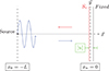Figure 1. One-dimensional problem of interaction of a normally incident elastic wave with a planar interface whose one face is fixed. The boundary nodes {x 0 = −L, x n  = 0} for finite differences method are illustrated.

2.1 Interface contact laws

CAN is notably modeled using contact laws. The simplest ones are: Unilateral contact law to mimic clapping (alternating opening and closure) and Coulomb law to mimic alternating stick/slip.

2.1.1 Unilateral contact law

Stated by Antonio Signorini in 1959 [29], this law describes the behavior of high-amplitude elastic waves when they interact with perfectly flat surfaces. However, it does not account for the roughness of the surfaces nor the phenomenon of adhesion. It primarily focuses on the “clapping” mechanism, which is an alternation of two states: contact or detachment. According to the convention illustrated in Figure 1, this law is stated as follows: if a static compression σ₀ is applied to each point on the contact surface (S_c) located at x = x_c = 0:

$$\begin{array}{c}\hfill \{\begin{array}{c}\text{1. Total normal stress on the surface:}\hfill \\ {\mathrm{\sigma n}}_{}(u(t,{\mathrm{xc}}_{}))+{\sigma }_0\le 0\hfill \\ \text{2. Normal displacement jump:}[{\mathrm{un}}_{}(t,{\mathrm{xc}}_{})]\le 0\hfill \\ \text{3.}{\mathrm{\sigma n}}_{}({\mathrm{un}}_{}(t,{\mathrm{xc}}_{}))\times [{\mathrm{un}}_{}(t,{\mathrm{xc}}_{})]=0,\forall {\mathrm{xc}}_{}\in {\mathrm{Sc}}_{}.\hfill \end{array}\end{array}$$(1)

The first line of this system ensures that only a compressive stress can exist at the interface; the second one indicates the non-penetration of the solid through the rigid surface, and when [u _n (t, x _c )] = (u _n ⁺ − u _n ⁻)(t, x _c )> 0 the interface is open (detachment with σ _n  + σ ₀ = 0), while the third ensures that the surface is either open or closed. The Unilateral Contact Law is illustrated in Figure 2a.

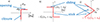Figure 2. Description of hypotheses used in the Unilateral contact law (a) and the Coulomb friction contact law (b, c); a: the supposed total normal stress versus the normal displacement jump – each half-line corresponds to an interface state : opened or closed –; in Coulomb law, tangential stress versus tangential displacement jump (b) and versus normal stress (c).

2.1.2 Coulomb friction law

The second law, known as Coulomb’s friction law, governs the interaction between the crack interface and the incident tangential stresses. This interface can be in one of two states: adherence or sliding. Its formulation involves the material’s coefficient of friction, denoted as C _f , as well as the normal stress σ _n (u(t, x _c )) + σ ₀ with σ ₀ being a static compression at the interface:

$$\begin{array}{c}\hfill \{\begin{array}{c}\text{Shear stress:}|\tau (u(t,{\mathrm{xc}}_{}))|\le {\mathrm{Cf}}_{}|{\mathrm{\sigma n}}_{}(u(t,{\mathrm{xc}}_{}))+{\sigma }_0|\hfill \\ \text{If}|\tau (u(t,{\mathrm{xc}}_{}))|<{\mathrm{Cf}}_{}|{\mathrm{\sigma n}}_{}(u(t,{\mathrm{xc}}_{}))+{\sigma }_0|\hfill \\ \Rightarrow \text{adherence: tangential jump}[{\mathrm{ut}}_{}(t,{\mathrm{xc}}_{})]=0\hfill \\ \text{If}|\tau (u(t,{\mathrm{xc}}_{}))|={\mathrm{Cf}}_{}|{\mathrm{\sigma n}}_{}(u(t,{\mathrm{xc}}_{}))+{\sigma }_0|\hfill \\ \Rightarrow \text{sliding:}\tau (u(t,{\mathrm{xc}}_{}))\times [{\mathrm{ut}}_{}(t,{\mathrm{xc}}_{})]\le 0.\hfill \end{array}\end{array}$$(2)

For a point on the crack located at x _c (see Figs. 2b and 2c), if the tangential stress |τ(u(t, x _c ))| is less than C _f |σ _n (u(t, x _c )) + σ ₀|, there is no sliding. The tangential displacement jump [u _t (t, x _c )] is zero. Conversely, when this inequality becomes an equality, sliding is initiated. In this situation, the tangential stress reaches a value equal to ±C _f |σ _n (u(t, x _c )) + σ ₀|, as long as sliding is possible.

2.2 Improved 1D analytical model

The 1D analytical model was developed by P. Blanloeuil in the work presented in the second chapter of his thesis [20] and the theoretical formulations are just briefly shown in appendix only for an incident longitudinal wave. We assume that the interface is planar and smooth to simplify the modeling. To represent the interaction plane wave/contact interface, we apply the principles of unilateral contact for incident normal stresses at the interface (L wave) and the Coulomb friction model for incident tangential stresses (T wave). The problem we study involves the reflection of the wave on an interface whose the non-insonified faceis a perfectly rigid and undeformable surface located at position x = 0, as illustrated in Figure 1.

The material is well-defined by its mechanical properties: a Young’s modulus E, a Poisson’s ratio ν and a mass density ρ.

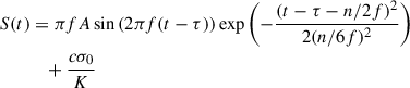
The acoustic source is located at x = −L and generates a wave, whether of type L or T, propagating along the x-axis. This source is initially established with an acoustic velocity at x = −L. It is set as n cycles of sine waves, which are windowed by a Gaussian envelope with a unit amplitude A and a standard deviation Δ, defined as Δ = n/(6f) (f denoting the frequency of the sine waves). Therefore, its form is given by:

$$\begin{array}{cc}\hfill S(t)& =\mathrm{\pi fA}sin(2\mathrm{\pi f}(t-\tau ))exp(-\frac{{(t-\tau -n/2f)}^2}{2{(n/6f)}^2})\hfill \\ \hfill & +\frac{c{\sigma }_0}{K}\hfill \end{array}$$(3)

with τ representing the time delay after the signal is emitted by the point source, and the term $\frac{c{\sigma }_0}{K}$ is included to account for a static compressive stress σ ₀, where K represents the stiffness model and c the propagation velocity. This source propagates throughout the space x, covering the interval [ − L, 0], following the formula:

$$\begin{array}{c}\hfill {\mathrm{ui}}_{\prime }^{}(x,t)=S(t-(x+L)/c).\end{array}$$(4)

The notation (′) represents a derivative with respect to time. The integration of this expression allows us to calculate the displacement of the incident wave, denoted as u _i .

The total displacement is calculated as the sum of the incident and reflected displacements, formulated as follows:

$$\begin{array}{c}\hfill u(x,t)={\mathrm{ui}}_{}(t-x/c)+{\mathrm{ur}}_{}(t+x/c).\end{array}$$(5)

Based on the existing theoretical formulation, we developed a code that allowed us to continuously monitor the state of the crack as a function of the type of incident wave at each instant. Blanloeuil noted, however about his own codes, that “It is therefore possible to obtain the solution to the contact problem semi-analytically, by constructing the solution in pieces. This involves finding the zeros of functions, which can be done using a numerical tool such as Maple. However, determining the times of transition between the contact and opened phases can be computationally expensive as the number of cycles increases; he therefore opted for a numerical solution”. In our model implemented here, the zero-finding is simply performed by finding the first next meshed time – showing change of functions sign – with a finer resolution δ t, likely smaller than what Blanloeuil intended. This optimization significantly improves the computational efficiency while maintaining the accuracy of the results. The block diagrams of the algorithms explaining the procedures are presented in Appendix A.

In addition to our analytical model, we have implemented a 1D numerical approach developed by P. Blanloeuil in his thesis [20], using the finite difference method (FDM) to solve the 1D propagation and scattering equations using the previous contact laws. The boundary nodes {x ₀ = −L, x _n  = 0} for finite differences method are illustrated in Figure 1 and the other nodes are equally meshed between them along the x-axis.

2.3 A preliminary 2D nonlinear analytical model

In this new investigation, our objective is to develop a two-dimensional (2D) model to address the contact problem and simulate the behavior of the crack under oblique incidence. We will continue to use the same parameters as in the one-dimensional (1D) case. However, in this instance, we will examine an oblique incident plane longitudinal wave (L) (see Fig. 3). The configuration of non-collinear waves mixing [30] which assumes two incident waves cannot be handled in this preliminary model. To simplify our study, we will also assume, as in the 1D case, that there will be no transmitted field to consider below the crack. This is a simplified hypothesis that should be removed in future improvements of the model.

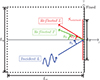Figure 3. 2D problem of interaction of an oblique elastic wave with a crack.

The simplified model proposed here assumes the existence of clapping only, neglecting sliding phenomena. An analytical solution is derived for the scattering problem of an obliquely incident wave on an interface, considering two distinct states: contact/adhesion (stick) and detachment (opened).

By applying the Helmholtz decomposition, we can express the reflected wave displacement field as follows:

$$\begin{array}{c}\hfill {\mathbf{ur}}_{}=\mathrm{\nabla \varphi }+\mathrm{\nabla },\psi .\end{array}$$(6)

In this equation, the scalar potential ϕ and the vector potential ψ describe the reflected L and T propagating waves, respectively. The L and T wavenumbers are denoted ${\mathrm{kL}}_{}=\frac{\omega }{{\mathrm{cL}}_{}}$ and ${\mathrm{kT}}_{}=\frac{\omega }{{\mathrm{cT}}_{}}$, where ω represents the wave angular frequency.

According to Snell’s law, the y component of the wave vector can be expressed as:

$$\begin{array}{c}\hfill \xi ={\mathrm{kL}}_{}sin({\mathrm{\theta L}}_{})={\mathrm{kT}}_{}sin({\mathrm{\theta T}}_{}).\end{array}$$(7)

The x component of the wave vector differs depending on the nature of the wave, and is expressed as:

$$\begin{array}{c}\hfill \alpha ={\mathrm{kL}}_{}cos({\mathrm{\theta L}}_{})\text{and}\beta ={\mathrm{kT}}_{}cos({\mathrm{\theta T}}_{}).\end{array}$$(8)

The two reflected longitudinal L and transversal T displacement fields can be expressed using the same analysis as that presented by Blanloeuil in 1D and summarized in Appendix A.

Since the incident wave propagates along x >  0 and y >  0, we can express the total displacement field as follows:

$$\begin{array}{c}\hfill \mathbf{u}(t,x,y)={\mathrm{ui}}_{}\left(\omega (t-\frac{\mathrm{\alpha \omega }}{}x-\frac{\mathrm{\xi \omega }}{}y)\right)\left(\begin{array}{c}cos{\mathrm{\theta L}}_{}\\ sin{\mathrm{\theta L}}_{}\end{array}\right)+{\mathbf{ur}}_{}(t,x,y).\end{array}$$(9)

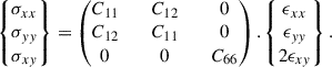
The constitutive laws allow us to relate the stresses to the displacements using the stiffness matrix of the assumed isotropic solid and the strain vector:

$$\begin{array}{c}\hfill \left\{\begin{array}{c}{\sigma }_{\mathit{xx}}\\ {\sigma }_{\mathit{yy}}\\ {\sigma }_{\mathit{xy}}\end{array}\right\}=\left(\begin{array}{ccc}{C}_{11}& C_{12}& 0\\ C_{12}& C_{11}& 0\\ 0& 0& C_{66}\end{array}\right).\left\{\begin{array}{c}{ϵ}_{\mathit{xx}}\\ {ϵ}_{\mathit{yy}}\\ 2{ϵ}_{\mathit{xy}}\end{array}\right\}.\end{array}$$(10)

The (C _{i j} ) denote the coefficients of the stiffness matrix and the (ϵ) are the normal and tangential strains.

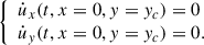
The Signorini and Coulomb laws will both be used. In the case of Adhesion/Contact (C), the mobile part of the crack is completely in contact with the fixed part and there is no friction. This means that the normal and tangential velocities (and displacements) are zero at the contact point, which can be formulated by the following equations for any point (0, y _c ) of the crack:

$$\begin{array}{c}\hfill \{\begin{array}{c}{\dot{u}}_x(t,x=0,y={\mathrm{yc}}_{})=0\hfill \\ {\dot{u}}_y(t,x=0,y={\mathrm{yc}}_{})=0.\hfill \end{array}\end{array}$$(11)

From this system, we can deduce the equations that relate the reflected velocity to the incident velocity, always at a point of the crack:

$$\begin{array}{c}\hfill \{\begin{array}{cc}{u}_{\mathit{rL}}^{\prime }(t,0,{\mathrm{yc}}_{})={\mathrm{DCL}}_{}^{}{\mathrm{ui}}_{\prime }^{}(t,0,{\mathrm{yc}}_{});\hfill & {\mathrm{DCL}}_{}^{}=\frac{cos({\mathrm{\theta L}}_{}+{\mathrm{\theta T}}_{})}{cos({\mathrm{\theta L}}_{}-{\mathrm{\theta T}}_{})}\hfill \\ u_{\mathit{rT}}^{\prime }(t,0,{\mathrm{yc}}_{})={\mathrm{DCT}}_{}^{}{\mathrm{ui}}_{\prime }^{}(t,0,{\mathrm{yc}}_{});\hfill & {\mathrm{DCT}}_{}^{}=\frac{-sin2{\mathrm{\theta L}}_{}}{cos({\mathrm{\theta L}}_{}-{\mathrm{\theta T}}_{})}.\hfill \end{array}\end{array}$$(12)

We can thus calculate the reflected velocity field at each point of the crack at each instant and then deduce the reflected displacement field than can also be propagated as plane waves in an area surrounding the crack if it is supposed to be large compared to the wavelength.

In the case of Detachment (D), the upper surface is free. This means that any stress applied to this surface is zero:

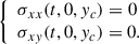$$\begin{array}{c}\hfill \{\begin{array}{c}{\sigma }_{\mathit{xx}}(t,0,{\mathrm{yc}}_{})=0\hfill \\ {\sigma }_{\mathit{xy}}(t,0,{\mathrm{yc}}_{})=0.\hfill \end{array}\end{array}$$(13)

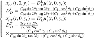
This is equivalent to the following system:

$$\begin{array}{c}\hfill \{\begin{array}{c}{u}_{\mathit{rL}}^{\prime }(t,0,{\mathrm{yc}}_{})={\mathrm{DDL}}_{}^{}{\mathrm{ui}}_{\prime }^{}(t,0,{\mathrm{yc}}_{});\hfill \\ {\mathrm{DDL}}_{}^{}=\frac{C_{66}sin2{\mathrm{\theta L}}_{}tan2{\mathrm{\theta T}}_{}-(C_{11}{cos}^2{\mathrm{\theta L}}_{}+C_{12}{sin}^2{\mathrm{\theta L}}_{})}{C_{66}sin2{\mathrm{\theta L}}_{}tan2{\mathrm{\theta T}}_{}+(C_{11}{cos}^2{\mathrm{\theta L}}_{}+C_{12}{sin}^2{\mathrm{\theta L}}_{})}\hfill \\ u_{\mathit{rT}}^{\prime }(t,0,{\mathrm{yc}}_{})={\mathrm{DDT}}_{}^{}{\mathrm{ui}}_{\prime }^{}(t,0,{\mathrm{yc}}_{});\hfill \\ {\mathrm{DDT}}_{}^{}=\frac{2{\mathrm{cT}}_{}sin2{\mathrm{\theta L}}_{}}{{\mathrm{cL}}_{}cos2{\mathrm{\theta T}}_{}}\hfill \\ \times \frac{(C_{11}{cos}^2{\mathrm{\theta L}}_{}+C_{12}{sin}^2{\mathrm{\theta L}}_{})}{C_{66}sin2{\mathrm{\theta L}}_{}tan2{\mathrm{\theta T}}_{}+(C_{11}{cos}^2{\mathrm{\theta L}}_{}+C_{12}{sin}^2{\mathrm{\theta L}}_{})}.\hfill \end{array}\end{array}$$(14)

We finally obtain the reflection coefficients for an incident plane wave in an elastic half-space on a free boundary. However, for a deeper understanding, we push our analysis further by taking the limit as angles θ _L and θ _T tend to zero in the systems of equations (12) and (14), which allows us to obtain the result of the one-dimensional case for normal incidence, while using a vectorial modeling (the reflected T wave is zero).

3 Results

3.1 Improved 1D analytical model

We conducted simulations using a longitudinal wavelet with a maximum amplitude of 9 nm over 5 sinusoidal cycles at a frequency of 1 MHz. The numerical calculations were performed over a domain of length L _x  = 5 cm, with a spatial resolution chosen to discretize the wavelength into 32 spatial steps Δx. The time step Δt was set to respect the CFL stability condition, with number c f l = 0.8.

A comparison between the semi-analytical model (blue) and the finite differences (FDM) model (red) was made for the normal stress and total displacement at the interface at x = 0 (Fig. 4). The reflected wave (analytically predicted) exhibit significant distortions compared to the incident wave. The spectra of the incident and total stresses (Fig. 4a) reveal new harmonic components in the reflected wave, characterized by multiples of the fundamental frequency.

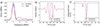Figure 4. Comparison between the analytical model (in blue) and the finite differences (FDM) model (in red): Normal stress (b) and total displacement (c) at the interface, at x = 0, with a static stress of σ 0 = −1 MPa. (a): spectrum of incident and total analytical normal stress.

The behavior of the interface well follows the unilateral contact law. The normal stress at the surface show plateaus at zero values during detachment phases, indicating no traction on the surface. The total normal displacement is zero during contact and negative during detachment.

While both models show similar behaviors, the FDM model generate numerical errors during sudden stress changes, particularly at the end of the second detachment phase (t ≈ 36.5 s). The analytical model demonstrated a faster computation time (at least 100 times faster for the studied configuration), making it preferable for larger simulations: indeed, the computation time is 0.025 s for the 1D analytical model and 2.95 s, 5.65 s and 12.95 s for respective CFL numbers equal to 0.8, 0.5 and 0.25 for the 1D numerical model. Calculation times are given in all the paper for a Dell Precision 3581 PC, 13th Gen i7-13800H, 2500 MHz, 14 cores, 20 logical processors, RAM 32 GB.

3.2 The preliminary 2D nonlinear analytical model

The flaw length is chosen as L _f  = 3 cm. We have first generated graphs (not shown here) illustrating the predicted normal stress at the surface as well as the displacements at the origin (0, 0) for different static stresses and different angles of incidence. We have noticed that no traction can be exerted on the surface, which explains the presence of plateaus at zero values, thus representing the detachment phase. This situation results in a loss of symmetry of the signal. Furthermore, it is important to emphasize that the third line inequality of the unilateral contact law is strictly respected when we perform the product of the normal stress by the normal displacement.

Then we have carried out a comparison of our 2D model with P. Blanloeuil’s Finite Elements Method (FEM) model [20]. The 2D FEM calculation configuration is shown in Figure 3.14 and Figure 3.15 of [20]. According to the description provided in his thesis, we have adopted an isotropic aluminum material (E = 69 GPa, ρ = 2700 kg/m³, C _f  = 0.8) for this study, subjected to a static compressive stress of σ ₀ = −0.15 MPa. We plot the profiles of total normal stress and shear stress at the center of the crack, considering two different angles of incidence, namely 0° and 25°. The results obtained are presented below: At normal incidence (1D case) (see Fig. 5), the analytical tangential stress is always zero (as supposed in the unilateral contact law). Note that the incident signal is not exactly specified in [20], which could explain the observed differences in the signals shapes predicted by the two models. Nevertheless, the two models predict similar maximal amplitudes and behaviors. Again the numerical model shows some instabilities (for instance the FEM tangential stress can be slightly non zero).

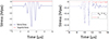Figure 5. Comparison between the analytical model (at left) and the Finite Elements Method (FEM) model (at right – Reproduced from [20]) for a normal incidence on a finite crack: Normal stress (in blue) and total displacement (in red) at the interface, at x = 0, with a static stress of σ 0 = −0.15 MPa.

When increasing the incident angle, for example at 25° (see Fig. 6), the tangential stress is neither zero (see Figs. 6b and 6c). This tangential stress is not enough to cause sliding for small angles for which the “clapping only” hypothesis is justified. When the crack opens, i.e., when the total normal stress becomes zero, the shear stress also cancels out to respect the free surface condition. The new simplified 2D model shows good agreement with finite elements. However, it should be noted that in P. Blanloeuil’s numerical model, oscillations around the equilibrium value are observed, which could be attributed to insufficient spatial discretization step. Despite these oscillations, Blanloeuil’s numerical model remains globally stable.

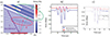Figure 6. 2D analytical simulation of the interaction of a longitudinal ultrasonic plane wave at 25° incidence with the normal to an interface with the bottom face fixed and including a crack of 30 mm length (represented by a red rectangle); (a): snapshot of the scattered field; normal and tangential stress as functions of time for the analytical model (b) and FEM model – Reproduced from [20] – (c).

The 2D analytical model has also allowed us to create animations presenting a sequence of maps of the (x, y) plane at different time instants, highlighting characteristic quantities such as displacement, velocity, and stress of the wave. These animations provide a visual representation that helps better understand the interaction mechanisms and interfacial contact. In Figure 6a, the back face of the interface has been taken fixed on both sides (at left and at right) of the crack and both the reflected longitudinal and transverse scattered by the interface and the crack can be displayed. For calculating and displaying the 2D animation of 790 snapshots (25° incidence – Fig. 6a) in a grid of 44 * 172 points (i.e., a total number of computation points of 5,98.10e6), the calculation time of the 2D analytical model is 28.13 s.

4 Conclusion

In this study, in the aim of modelling contact acoustic nonlinearity at a planar interface, we optimized a 1D analytical model based on the unilateral contact and the Coulomb friction law, achieving a tenfold speed advantage over finite differences models. We then proposed a preliminary 2D analytical model for nonlinear scattering of elastic waves from finite cracks, demonstrating good agreement with Finite Element Methods (FEM) for low incident angles. Future work will focus on refining the 2D model’s hypotheses to extend its validity and incorporating a more realistic description of nonlinear interfacial phenomena. These advancements will enhance our understanding of wave-crack interactions and improve the accuracy of NDT simulations. Indeed, the perspectives of this work will be to progressively develop a simulation tool of a non-linear ultrasonic crack measurement system that could then be experimentally tested on real cracks.

Acknowledgments

Authors thank Malo Lavoué for his preliminary work on the topics and Philippe Blanloeuil for their discussions on his Ph.D. thesis works.

Funding

The internship of Zakaria Yajioui has been funded by CEA.

Conflicts of interest

Authors declare no Conflict of Interest.

Data availability statement

The research data associated with this article are included within the article.

References

Appendix A

1D analytical model

In this appendix, we detail our 1D analytical model. We use a functional diagram to illustrate its behavior for an incident L wave.

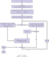Figure A.1. Functional diagram of the 1D analytical model.

All Figures

	Figure 1. One-dimensional problem of interaction of a normally incident elastic wave with a planar interface whose one face is fixed. The boundary nodes {x 0 = −L, x n  = 0} for finite differences method are illustrated.
In the text

	Figure 2. Description of hypotheses used in the Unilateral contact law (a) and the Coulomb friction contact law (b, c); a: the supposed total normal stress versus the normal displacement jump – each half-line corresponds to an interface state : opened or closed –; in Coulomb law, tangential stress versus tangential displacement jump (b) and versus normal stress (c).
In the text

	Figure 3. 2D problem of interaction of an oblique elastic wave with a crack.
In the text

	Figure 4. Comparison between the analytical model (in blue) and the finite differences (FDM) model (in red): Normal stress (b) and total displacement (c) at the interface, at x = 0, with a static stress of σ 0 = −1 MPa. (a): spectrum of incident and total analytical normal stress.
In the text

	Figure 5. Comparison between the analytical model (at left) and the Finite Elements Method (FEM) model (at right – Reproduced from [20]) for a normal incidence on a finite crack: Normal stress (in blue) and total displacement (in red) at the interface, at x = 0, with a static stress of σ 0 = −0.15 MPa.
In the text

Figure 6. 2D analytical simulation of the interaction of a longitudinal ultrasonic plane wave at 25° incidence with the normal to an interface with the bottom face fixed and including a crack of 30 mm length (represented by a red rectangle); (a): snapshot of the scattered field; normal and tangential stress as functions of time for the analytical model (b) and FEM model – Reproduced from [20] – (c).

In the text

	Figure A.1. Functional diagram of the 1D analytical model.
In the text

References

- M. Darmon: Special issue on ultrasonic modeling for non-destructive testing. Applied Sciences 14 (2024) 2008. [Google Scholar]
- Civa Software Website: http://www.extende.com/. [Google Scholar]
- M. Darmon, A. Ferrand, V. Dorval, S. Chatillon, S. Lonné: Recent modelling advances for ultrasonic TOFD inspections. AIP Conference Proceedings 1650 (2015) 1757–1765. [Google Scholar]
- A. Ferrand, M. Darmon, S. Chatillon, M. Deschamps: Modeling of ray paths of head waves on irregular interfaces in TOFD inspection for NDE. Ultrasonics 54 (2014) 1851–1860. [Google Scholar]
- G. Toullelan, R. Raillon, S. Chatillon, V. Dorval, M. Darmon, S. Lonné: Results of the 2015 UT modeling benchmark obtained with models implemented in CIVA. AIP Conference Proceedings 1706 (2016) 190001. [Google Scholar]
- R. Raillon, S. Bey, A. Dubois, S. Mahaut, M. Darmon: Results of the 2009 UT modeling benchmark obtained with CIVA: responses of notches, side-drilled holes and flat-bottom holes of various sizes. AIP Conference Proceedings 1211 (2010) 2157–2164. [Google Scholar]
- V. Zernov, L. Fradkin, M. Darmon: A refinement of the kirchhoff approximation to the scattered elastic fields. Ultrasonics 52 (2012) 830–835. [Google Scholar]
- M. Darmon, V. Dorval, A. Kamta Djakou, L. Fradkin, S. Chatillon: A system model for ultrasonic NDT based on the physical theory of diffraction (PTD). Ultrasonics 64 (2016) 115–127. [Google Scholar]
- A. Imperiale, S. Chatillon, M. Darmon, N. Leymarie, E. Demaldent: UT simulation using a fully automated 3D hybrid model: application to planar backwall breaking defects inspection. AIP Conference Proceedings 1949 (2018) 050004. [Google Scholar]
- M. Darmon, G. Toullelan, V. Dorval: An experimental and theoretical comparison of 3D models for ultrasonic non-destructive testing of cracks: Part I, embedded cracks. Applied Sciences 12 (2022) 5078. [Google Scholar]
- L.J. Fradkin, A.K. Djakou, C. Prior, M. Darmon, S. Chatillon, P.-F. Calmon: The alternative Kirchhoff approximation in elastodynamics with applications in ultrasonic nondestructive testing. The ANZIAM Journal 62 (2020) 406–422. [Google Scholar]
- V. Zernov, L. Fradkin, A. Gautesen, M. Darmon, P. Calmon: Wedge diffraction of a critically incident Gaussian beam. Wave Motion 50 (2013) 708–722. [Google Scholar]
- L.J. Fradkin, M. Darmon, S. Chatillon, P. Calmon: A semi-numerical model for near-critical angle scattering. The Journal of the Acoustical Society of America 139 (2016) 141–150. [Google Scholar]
- V. Dorval, A. Imperiale, M. Darmon, E. Demaldent, J.-M. Hénault: FEM-based simulation tools for ultrasonic concrete inspection. E-J. Nondestruct. Test., 27, 2022. [Google Scholar]
- S. Chehade, A. Kamta Djakou, M. Darmon, G. Lebeau: The spectral functions method for acoustic wave diffraction by a stress-free wedge: theory and validation. Journal of Computational Physics 377 (2019) 200–218. [Google Scholar]
- S. Chehade, M. Darmon, G. Lebeau: 2D elastic plane-wave diffraction by a stress-free wedge of arbitrary angle. Journal of Computational Physics 394 (2019) 532–558. [Google Scholar]
- S. Chehade, M. Darmon, G. Lebeau: 3D Elastic plane-wave diffraction by a stress-free wedge for incident skew angles below the critical angle in diffraction. Journal of Computational Physics 427 (2021) 110062. [Google Scholar]
- M. Darmon, V. Dorval, F. Baqué: Acoustic scattering models from rough surfaces: a brief review and recent advances. Applied Sciences 10 (2020) 8305. [Google Scholar]
- F. Shi, W. Choi, M.J.S. Lowe, E.A. Skelton, R.V. Craster: The validity of Kirchhoff theory for scattering of elastic waves from rough surfaces. Proceedings of the Royal Society A: Mathematical, Physical and Engineering Sciences 471 (2015) 20140977. [Google Scholar]
- P. Blanloeuil: Analyse de la non-linéarité acoustique de contact pour l’ évaluation et le contrôle non destructif. Ph.D. thesis, Université Bordeaux 1, 2013. [Google Scholar]
- A. Perrin: Ultrasons non linéaires pour la caractérisation de fissures fermées dans les matériaux métalliques, 2024. [Google Scholar]
- J.M. Richardson: Harmonic generation at an unbonded interface – I. Planar interface between semi-infinite elastic media. International Journal of Engineering Science 17 (1979) 73–85. [Google Scholar]
- P. Blanloeuil, L.R.F. Rose, M. Veidt, C.H. Wang: Analytical and numerical modelling of wave scattering by a linear and nonlinear contact interface. Journal of Sound and Vibration 456 (2019) 431–453. [Google Scholar]
- S. Biwa, S. Nakajima, N. Ohno: On the acoustic nonlinearity of solid-solid contact with pressure-dependent interface stiffness. Journal of Applied Mechanics 71 (2004) 508–515. [Google Scholar]
- C. Pecorari: Nonlinear interaction of plane ultrasonic waves with an interface between rough surfaces in contact. The Journal of the Acoustical Society of America 113 (2003) 3065–3072. [Google Scholar]
- A. Perrin, C. Gueudré, M.A. Ploix, G. Corneloup, T.J. Ulrich, L. Beardslee, P. Recolin, C. Payan: Closed cracks characterization in a steel sample applying a pump probe waves ultrasonic method. Journal of Nondestructive Evaluation, Diagnostics and Prognostics of Engineering Systems 7 (2024) 041002. [Google Scholar]
- A. Meziane, P. Blanloeuil, D. Nouira, L. Baillet, F. Massi: Numerical analysis of a one-dimensional nonlinear wave scattering at a contact interface with damageable adhesion and unilateral contact. Wave Motion 122 (2023) 103182. [Google Scholar]
- A. Di Bella, M. Scalerandi, A.S. Gliozzi, F. Bosia: Adhesion and plasticity in the dynamic response of rough surfaces in contact. International Journal of Solids and Structures 216 (2021) 17–29. [Google Scholar]
- A. Signorini: Questions on Nonlinear and Semilinear Elasticity. Rendiconti di matematica e delle sue applicazioni, 1959. Available at: http://www.scienzadellecostruzioni.co.uk/Documenti/Signorini-Prima.pdf. [Google Scholar]
- L.R.F. Rose, P. Blanloeuil, M. Veidt, C.H. Wang: Analytical and numerical modelling of non-collinear wave mixing at a contact interface. Journal of Sound and Vibration 468 (2020) 115078. [Google Scholar]