


| Issue |
Acta Acust.
Volume 10, 2026
|
|
|---|---|---|
| Article Number | 65 | |
| Number of page(s) | 16 | |
| Section | Room Acoustics | |
| DOI | https://doi.org/10.1051/aacus/2026060 | |
| Published online | 24 July 2026 | |
Scientific Article
Interlaboratory Comparison and Analysis of Bidirectional Scattering Coefficients for Various Surfaces
1
Institute for Hearing Technology and Acoustics, RWTH Aachen University, Aachen, Germany
2
School of Architecture, Design and Planning, The University of Sydney, Sydney, Australia
3
Individualized Production, RWTH Aachen University, Aachen, Germany
* Corresponding author: This email address is being protected from spambots. You need JavaScript enabled to view it.
Received:
16
December
2025
Accepted:
16
June
2026
Abstract
Accurate modeling of acoustic scattering is essential for realistic sound-propagation simulations in architectural environments. Traditional random-incidence models fail to represent directional scattering from structured surfaces, motivating the need for detailed bidirectional datasets. A reproducibility analysis of random-incidence and bidirectional scattering coefficient (BSC) measurements was conducted across two laboratories (RWTH Aachen University and The University of Sydney) using different free-field setups and two control surfaces–a 1D-sinusoidal and a 2D-rectangular profile. Measurements were compared with diffuse-field measurements (ISO 17497-1) and numerical simulations replicating the physical setups. Both laboratories produced consistent random-incidence scattering coefficients and BSCs for the 1D-sinusoidal surface. The 2D-rectangular surface showed larger deviations, attributed to edge effects and setup differences. Additional surfaces–including singular objects, random and modular geometries, and small-scale building façade elements–were measured or simulated. The method reliably captures directional scattering across various surface types. Setup geometry, edge effects, and signal-to-noise ratio were identified as key accuracy factors. The resulting coefficients together with its surface and setup descriptions provide a standardized foundation for future acoustic simulations and architectural applications.
Key words: Bidirectional scattering coefficients / Random-incidence scattering / Acoustic measurements / Architectural acoustics / Surface scattering database
© The Author(s), Published by EDP Sciences, 2026
 This is an Open Access article distributed under the terms of the Creative Commons Attribution License (https://creativecommons.org/licenses/by/4.0), which permits unrestricted use, distribution, and reproduction in any medium, provided the original work is properly cited.
1 Introduction
Accurate prediction and modeling of scattering in sound propagation simulations are essential for various acoustic applications. Scattering is typically modeled by dividing reflected sound into specular and diffuse components [1, 2]. The specular reflection mirrors the incidence angle across the surface normal, while diffuse reflections are modeled using Lambert’s cosine law. Additionally, the scattering coefficients are usually averaged over all incident angles. This random-incidence scattering coefficient is typically measured in a reverberation room according to ISO 17497-1 [3]. Databases of scattering coefficients are rare compared to absorption coefficients. Nevertheless, Cox and d’Antonio [1] and Vorländer [4, 5] measured or collected several random-incidence scattering coefficients.
However, random-incidence and Lambertian scattering models have limitations, particularly for non-stochastic surfaces such as periodic structures. These surfaces scatter sound in directionally distinct ways determined by their geometry [6], a behavior that conventional models fail to capture adequately, as they average over incoming directions and reduce complex scattering patterns to simplified Lambertian reflections.
This limitation is a source of errors since many acoustic environments, including rooms and urban spaces, feature inherently periodic surfaces. Building façades, in particular, can introduce significant scattering effects that dominate the acoustic environment [7–9]. The relevant scattering behavior should be considered within the audible wavelength range (15.6 mm ≤ λ ≤ 17 m) and mapped onto corresponding architectural scales [10]. In practice, progressively smaller architectural features–from large-scale vertical composition down to material texture–become acoustically significant as the wavelength decreases [10]. This wavelength-scale relationship provides a guideline for categorizing surface structures according to the architectural dimensions at which their scattering effects emerge.
To address the limitations of angular averaging, the bidirectional reflectance distribution function (BRDF) is often used in optics to describe the directional scattering of light from surfaces [11]. In acoustics, a similar concept can be used in geometrical sound propagation, combining absorption and scattering. For example, Siltanen et al. [12] derived BRDFs from random-incidence scattering and absorption coefficients assuming Lambertian scattering, due to the lack of measured acoustic BRDFs or directional scattering data. Binek et al. [13] calculated BRDFs from diffusers based on reflected sound pressure determined by the Fresnel diffraction method. Hargreaves [14] introduced a method to measure BRDFs using Near-Field Acoustical Holography (NAH) based on 2D-BEM simulation.
Brandao et al. [15] determined the far-field directivity of singular diffusors based on near-field measurements and plane-waves expansion. Recently, the bidirectional scattering coefficients (BSCs) were introduced to describe directional scattering independent of surface absorption [16]. The BSC describes the energy scattered into each direction depending on the incident direction. Heimes and Vorländer [16] have determined the BSC of a 1D-sinusoidal surface using a free-field measurement setup in Aachen. Additionally, the random-incidence scattering coefficients were derived from the BSCs and compared to previous diffuse-field measurements [2] according to ISO 17497-1 [3] and numerical simulations. The numerical simulation served as a digital twin of the measurement setup, and an optimal numerical setup to eliminate the geometrical effects for the setup.
At the University of Sydney, Cabrera et al. [17] developed a high-density hemispherical loudspeaker array for sound-field reproduction. This facility can be employed to obtain BSCs in a reciprocal operation mode.
In this paper, we present a dataset of measured bidirectional scattering coefficients (BSCs) as well as random-incidence scattering coefficients (RSC) for a range of surface geometries. Measurements were carried out in two laboratories–located in Sydney, Australia [17], and Aachen, Germany [16]. To evaluate reproducibility, two control surfaces–a one-dimensional sinusoidal profile and a two-dimensional rectangular profile–were measured in both laboratories. These measurements were further compared with diffuse-field data obtained in accordance with ISO 17497-1:2004 [3] and with numerical simulations replicating the respective physical setups. Additionally, we determined the BSC through physical measurements or numerical simulations for a variety of structures, such as singular objects, random and modular geometries, and small-scale building façade elements. The resulting BSCs and RSCs together with its surface properties are compiled into an openly accessible and extensible database and it is intended to support future research on acoustic scattering. Because the methodology is formulated in terms of relative frequency scaling, the techniques and results are applicable broadly and can be interpreted for a wide range of indoor and outdoor surfaces.
2 Free-field data acquisition
The reflected sound pressures were determined for several surfaces, including reference surfaces [16]. The free-field measurements were carried out in two laboratories: one located in Aachen, Germany, and the other in Sydney, Australia. The setup used in Aachen closely follows the configuration described in previous work [16], whereas the setup in Sydney is based on a high-density hemispherical loudspeaker array [17] in reciprocal operation mode.
2.1 Lab 1: measurement Aachen
The measurement setup in Aachen was arranged in a hemi-anechoic chamber (Fig. 1). The sample was placed 2 m above the ground on a turntable. A movable loudspeaker arc (radius 1.2 m) equipped with 36 Tang Band W1-2025SA (1′′) drivers in custom 0.05 l enclosures [18], and a stationary microphone arc (radius 1 m) comprising 32 Sennheiser KE4 electret microphones, were used, following the configuration described in [16]. The pressure impulse responses were measured using the Multiple Exponential Sweep Method [19] at a sampling rate of fs = 48 kHz with a frequency range from 1 kHz to 24 kHz.
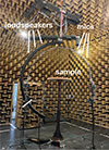 |
Figure 1. Measurement setup in Aachen, Germany. |
Two measurement series were conducted, during which temperature and relative humidity were recorded. The first series took place on 9 August 2024, with an average temperature of 23.38 ° C and a relative humidity of 60.25%. The maximum variations observed during this session were 0.11 ° C in temperature and 1.84% in relative humidity. The second series was conducted between 25 February and 28 February 2025. The mean temperature and relative humidity were 20.84 ° C and 39.14%, respectively. The maximum changes in temperature and relative humidity during this interval were 0.31 ° C and 1.22%, respectively. The sinusoidal surface 1 was measured in both series, while all other surfaces were measured once.
Azimuthal incidence angles were sampled in increments of 45°, 15°, and/or 10°, up to a maximum of 90° or 180°, depending on the symmetry of the surface under investigation. For each measurement, the total duration was 103 min, corresponding to angular increments of 10° up to 90°, for example.
2.1.1 Post-processing
The impulse response measurement in Aachen contained the direct sound, the reflection of the sample and reflections from ground and measurement setup. The reflected sound pressure of the sample was isolated by first measuring the free-field response–i.e., the direct sound–without any sample or supporting structure present. To eliminate floor reflections, the direct sound was windowed using a right-sided Hann window with a length of 10 ms. This windowed direct sound was then subtracted from the measured sound pressure using the optimized subtraction method described in [16].
Following subtraction, the reflected sound pressure was further processed applying a symmetric Hann window. The window limits were determined based on the positions of each of the sources and receivers, with the shortest and longest expected edge reflections defining the window boundaries. An additional margin of 10 samples was included at both the beginning and end of the window to ensure complete capture of the reflection tails.
The signal-to-noise ratio (SNR) was evaluated for each measurement series (Fig. 2). The SNR was calculated from the specular reflected sound pressure of the flat reference surfaces relative to the noise in the free-field measurements. The procedure followed the SNR calculation defined in ISO 17497-2:2012 [20] and described in [16]. As in [16], the 40 dB signal-to-noise ratio (SNR) recommended in [20] was not achieved. Instead, a minimum SNR of approximately 20 dB was obtained for incident angles below 60°. The higher SNR above 60° is due to the close arrival times of the direct sound and its reflection, which makes them difficult to separate.
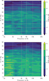 |
Figure 2. SNR for the first (top) and second (bottom) measurement series in Aachen. |
After the reflected components were isolated, the bidirectional scattering coefficients were computed, followed by the derivation of the random-incidence scattering coefficients as described in [16]. Additionally, the normalized directional diffusion coefficients were calculated based on the isolated reflected sound pressure [20].
2.2 Lab 2: measurement Sydney
The measurement in Sydney took place between 2 December 2024 and 6 December 2024. These measurements included all surfaces described below, while sinusoidal surface 1 was measured twice, with a 90° shift.
It was conducted using a high-density hemispherical loudspeaker array [17], which consisted of 196 electrodynamic loudspeakers arranged in an icosahedral pattern with a radius of approximately 2.15 m (Fig. 3). The loudspeakers used are 102 mm spherical Anthony Gallo ‘Nucleus Micro’. The sample was placed at the center of the array on a fixed stand. All loudspeakers except for one were used as receivers in a reciprocal configuration by disconnecting them from the amplifier and connecting them to the microphone preamplifier. This process was automated using a custom-built switching matrix controlled by software (Fig. 4). This resulted in a missing receiver position at the incidence angle, because this loudspeaker was sending instead of receiving.
 |
Figure 4. Hardware setup for a single channel of the reciprocal measurement system used in Sydney. |
Impulse responses were measured using the exponential sweep method with a sampling rate of fs = 44.1 kHz and a frequency range of f ∈ [1 kHz, 20 kHz]. The temperature and relative humidity were recorded during the measurement, with an average temperature of 28.91 ° C and a relative humidity of 36.03%. The maximum changes in temperature and relative humidity during this interval were 4.90 ° C and 10.30%, respectively.
Due to technical issues, seven source channels (64, 128, 167, 179, 180, 195, 196) and one receiver channel (59) were not operational during the measurements.
The total measurement duration for all 196 incident positions was approximately 20 min.
2.2.1 Post-processing
The post-processing procedure closely followed the approach described for the Aachen measurements in Section 2.1.1, with the following key differences:
Prior to post-processing, the impulse responses were resampled to account for significant fluctuations in temperature and humidity, which led to variations in the speed of sound ranging from 347.2 m/s to 350.0 m/s. The correction was based on the speed of sound calculated from the ideal gas law [21].
Unlike in the Aachen setup, the direct sound was windowed using a right-sided Hann window ranging up to 30 ms. This upper limit was more extended than in the Aachen configuration due to the larger dimensions of the measurement environment.
To compensate for the malfunctioning input and output channels, the reciprocity principle was applied. For each non-functional input channel, the corresponding output channel data was used, and vice versa for each non-functional output channel.
The SNR was calculated based on the specular reflected sound pressure of the reference surfaces relative to the noise in the free-field measurement, as described in Section 2.1.1. The reflected sound pressure for the measurement series in Sydney (Fig. 5) showed a lower SNR compared to the Aachen measurements, primarily because of the limited sensitivity of the loudspeakers in receiving mode. These transducers did not have a flat transfer function in receiving mode, which negatively affected the measurement quality. For ϑs = 0°, no data was measured because the specular reflection from the top-pole loudspeaker returned directly to the same loudspeaker, which cannot transmit and receive simultaneously.
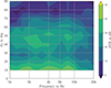 |
Figure 5. SNR for the measurement series in Sydney. |
After isolating the reflected sound pressure, we calculated the bidirectional scattering coefficients and then derived the random-incidence scattering coefficients as described in [16]. Additionally, the normalized directional diffusion coefficients were calculated based on the isolated reflected sound pressure [20].
2.3 Numerical simulation of the measurement setup
To compare the measurements obtained from the two laboratories, numerical simulations were conducted as “digital twins” of the measurement setups. Numerical simulations were also performed for an optimal configuration derived from [16], representing idealized geometrical conditions that cannot be realized in practice:
-
Aachen geometry: Point source and receiver positions matched those of the measurement configuration used in Aachen (Fig. 6a).
-
Sydney geometry: Point source and receiver positions matched those of the measurement configuration used in Sydney (Fig. 6b).
-
Optimal geometry (reference): The incident sound field was modeled as a plane wave with incident directions represented by a Gaussian sampling of order 21 at a quarter hemisphere (Fig. 6c). As in [16], the receivers were arranged as an equal area sampling of 23 328 points at a radius of 50 m to ensure far-field condition.
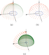 |
Figure 6. All geometrical setups with the sample ([-,mplBlue,solid,line width = 0.9pt](0,0) – (3mm,0);). (a) The measurement setup in Aachen with loudspeaker positions ([-,mplRed,solid,line width = 0.9pt](0,0) – (3mm,0);) and the microphone arc ([-,mplGreen,solid,line width = 0.9pt,opacity=0.8](0,0) – (3mm,0);) resulting in a total receiver array ([-,mplGreen,solid,line width = 0.9pt,opacity=0.4](0,0) – (3mm,0);) after the measurement procedure. (b) The measurement setup in Sydney with loudspeaker positions ([-,mplRed,solid,line width = 0.9pt](0,0) – (3mm,0);). (c) The optimal far-field simulation setup with the incidence plane waves in ([-,mplRed,solid,line width = 0.9pt](0,0) – (3mm,0);) and the receiver positions ([-,mplGreen,solid,line width = 0.9pt,opacity=0.8](0,0) – (3mm,0);). |
In all cases, the sample diameter was set to 80 cm, matching the diameter used in the reverberation room measurements in accordance with [3]. Additional surface geometries were also simulated to expand the dataset.
The simulations were carried out using the Boundary Element Method (BEM) solver Mesh2scattering [22], which is designed for acoustic scattering problems. This solver is built upon Mesh2HRTF [23] and utilizes the numerical core NumCalc [24]. All simulations were performed following the methodology described in [16].
The simulations were conducted over the frequency range from 1 kHz to 20 kHz, with 9 frequency bins per octave. The speed of sound was set to be 343.2 m/s. Triangular surface meshes were generated for three maximum frequency limits (5 kHz, 10 kHz, and 20 kHz), using a maximum edge length of λ/6, where λ denotes the wavelength of sound in air at the corresponding frequency limit.
2.3.1 Post-processing
Because the direct sound was excluded in the numerical simulation, the reflected sound pressure was directly used to calculate the bidirectional scattering coefficients and their random-incidence scattering coefficients as described in [16]. Additionally, the normalized directional diffusion coefficients were calculated using the isolated reflected sound pressure [20].
3 Diffuse-field data acquisition
For comparison, also the random-incidence scattering coefficients were directly measured according to ISO 17497-1:2004 [3] independently in Aachen and Sydney. In both laboratories, small-scale reverberation chamber measurements were conducted. The valid frequency range for these small-scale measurements ranges from N ⋅ 100 Hz to N ⋅ 5000 Hz, where N is the physical scale factor of the reverberation chamber.
3.1 Lab 1: measurement Aachen
Figure 7 shows the first small-scale reverberation chamber, which is placed at the Institute for Hearing Technology and Acoustics, RWTH Aachen University in Germany. The reverberation room has the dimensions of 1.5 m × 1.2 m × 0.95 m with hemispherical boundary diffusers derived in [25]. This leads to a volume of Vroom = 1.67 m3 and a surface area of Sroom = 9.05 m2, including the effect of the diffusers. This leads to a physical scale factor of N = 5, resulting in a valid frequency range of 500 Hz–25 kHz. All samples had a diameter of 0.8 m, and were flush-mounted on a turntable, as shown in Figure 7. All surfaces were measured twice.
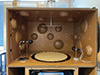 |
Figure 7. Small-scale reverberation room in Aachen, Germany. |
Two source positions and two microphones (GRAS Typ 40BF 1/4′′ freefield) were used. The sources consist of a custom-built dodecahedron with a diameter of 90 mm and 12 Föön dome tweeters. The microphones were moved in rotation and height by a motor to three motor positions. This leads to two source and six receiver positions. Impulse responses were measured using the exponential sweep method with a sampling rate of f s = 96 kHz and a frequency range from 2 kHz to 25 kHz. The higher lower frequency limit was selected as scattering starts at 2.5 kHz.
3.2 Lab 2: measurement Sydney
Figure 8 shows the second small-scale reverberation chamber, which is placed at the School of Architecture, Design and Planning, The University of Sydney in Australia. It is a rectangular room with unequal edge lengths of a Volume of Vroom = 0.972 m3 and a surface area of Sroom = 6.044 m2, leading to a physical scale factor of N = 6 and a valid frequency range of 600 Hz–30 kHz.
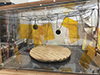 |
Figure 8. Small-scale reverberation chamber in Sydney, Australia. |
Two source positions and six 1/4 inch microphones were used. The source is a Dr.Three 3D loudspeaker. All samples had a diameter of 0.78 m, and were mounted on a turntable, as shown in Figure 8. Each surface was measured once. Impulse responses were measured using the exponential sweep method with a sampling rate of fs = 192 kHz and a frequency range from 1.5 kHz to 30 kHz. The frequency range was changed compared to the theoretical validity to meet the SNR requirements.
3.3 Measurement and post-processing
Following ISO 17497-1:2004 [3], four measurement conditions were acquired in both laboratories:
-
Condition 1: static base plate without sample.
-
Condition 2: static base plate with sample.
-
Condition 3: rotating base plate without sample, measured at 72 angular positions over a full 360° rotation.
-
Condition 4: rotating base plate with sample, measured at 72 angular positions over a full 360° rotation.
For measurement conditions 3 and 4, the impulse responses corresponding to the individual angular positions were summed over the complete rotation. This results in a set of impulse responses for each source-receiver pair and measurement condition.
Initially, the recorded impulse responses were truncated to remove the effects of loudspeaker non-linearities. Subsequently, all impulse responses were filtered into one-third-octave bands over the measured frequency range using the Python package pyfar [26].
The reverberation time was then estimated for each source-receiver pair and measurement condition using the Python package pyrato [27]. To estimate the energy decay curve, the noise level was determined from the last 5% of each impulse response. The squared noise was then subtracted from the squared impulse responses following the method defined by Chu [28]. The impulse responses were then truncated at the intersection point of the decay curve and the noise floor, as described by Lundeby et al. [29].
The energy decay curve was calculated, including the correction term defined by Guski and Vorländer [30]. The reverberation time T 15 was derived using linear regression in accordance with ISO 17497-1:2004 [3] and ISO 3382 [31]. The resulting reverberation times were averaged over all source-receiver positions. The speed of sound was calculated using the ideal gas law [21] based on the averaged temperature and relative humidity for each condition. Similarly, air attenuation was calculated following ISO 9613-1:1993 [32]. Finally, the scattering and absorption coefficients were calculated based on ISO 17497-1:2004 [3].
4 Investigated surfaces
This section presents the surfaces investigated and analyzed in this work and the structure of the resulting open dataset. A total of 28 surfaces were measured and/or simulated, covering a broad range of geometries relevant to architectural and environmental acoustics (Fig. 9).
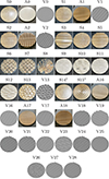 |
Figure 9. Sample identifiers and images of the selected surfaces, with singular objects highlighted with *. Large images are available in the dataset [33]. |
4.1 Surface organization and categorization
Each measured or simulated sample is assigned a unique sample identifier, which consists of a letter indicating the origin of the sample and a number indicating the surface identifier. The origin of the sample indicates whether it is measured in Aachen (A), in Sydney (S), or simulated numerically (V). The surface identifier is a unique identifier starting from 0 for the flat reference plate, followed by 1 for the first surface, and so on. The sample identifier and an image of each sample are presented in Figure 9.
The surfaces are categorized into two main types: regular standard (nominally infinitely extended) surfaces and individual objects. While the majority of samples represent standard surfaces suitable for general architectural applications, two special cases (Surface 14 and 15) represent individual objects. These were included to demonstrate the capability of our measurement methodology to accommodate isolated elements as well. However, it is important to note that such individual objects cannot be employed in the same standardized manner as extended architectural surfaces.
4.2 Control surfaces
Surfaces 1 and 2 were selected as control surfaces. They comprise a one-dimensional sinusoidal surface (Surface 1) and a two-dimensional rectangular surface (Surface 2). These surfaces were chosen to represent a wide range of surface characteristics [5], including one-dimensional rounded and two-dimensional angular geometries. In addition, the one-dimensional sinusoidal surface has been investigated in previous studies [2], and an analytical solution is available for this geometry [34].
Both control surfaces were characterized through experimental measurements conducted in both laboratories as well as by numerical simulations. In addition to simulations using the optimal setup, the control surfaces were also simulated using the specific geometrical configurations of the Aachen and Sydney laboratories (Figs. 6a and 6b), denoted as VA and VS for Aachen and Sydney, respectively.
4.3 Surface selection
In addition to the control surfaces, a diverse range of 26 surfaces was selected to cover various geometries commonly encountered in architectural and environmental acoustics. These surfaces were either measured in one of the two laboratories and/or simulated numerically. To illustrate the applicability of different surface types, a representative selection of examples is discussed.
These include surfaces with periodic corrugations of size Λ in one or two dimensions as well as angular and rounded surfaces.
For Surfaces 1 and 21 analytical solutions are known [34, 35]. Furthermore, Surface 21 was measured in a diffuse reflection example scene of a Benchmark for Room Acoustical Simulation (BRAS) [36].
Modular surfaces, such as Surfaces 6–8, consist of triangular prisms in different arrangements. Each element is formed by bisecting a cube (45 mm edge length) along the diagonal of one of its square faces. Surface 6 is identical to Surface 7, but includes additional elements mounted on the surface.
The dataset also includes samples derived from real building façades, such as:
-
the Refugee Quarters in Geneva, Switzerland (Surface 16) [10, 37],
-
the Preston Bus Station in the United Kingdom (Surfaces 17 and 18) [10, 37],
-
the Institute for Hearing Technology and Acoustics in Aachen, Germany (Surface 22) [38],
-
the BLB building in Aachen, Germany (Surface 23) [38], and
-
the Ainsworth Building in Sydney, Australia (Surface 24) [7].
These surfaces represent different architectural scales [10]. First, the bay division scale (Surfaces 18 and 22–24) represents the macro structure of the surface, while the cladding scale (Surfaces 16–17) covers the micro scale.
Commonly used diffuser surfaces are also included in the dataset, such as the Quadratic Residue Diffusor (QRD) [1] represented by Surface 25, and the Maximum Length Sequence (MLS) diffusor represented by Surface 3.
Additionally, randomly structured surfaces are included in the dataset, such as Surface 26, which consists of randomly distributed hemispheres with 50% surface coverage, as previously measured by de Avelar Gomes et al. [39].
Different non-rigid surfaces are also included (Surfaces 9–12) to evaluate the applicability of the measurement method to absorbing surfaces. These samples are made primarily of polystyrene foam, which increases absorption and consequently reduces the SNR in the measurements. To mitigate this effect, Surface 10 is coated with an additional layer of clay to reduce absorption. Surface 12 combines polystyrene with sound-reflecting wood, resulting in lower overall absorption compared to the fully foam-based configurations.
5 Laboratory comparison
We now discuss the results of the comparisons of the control surfaces in Aachen and Sydney as well as their digital twins as discussed in Sections 2 and 3. These results are also compared with the simulation results under optimal conditions and for the 1D-sinusoidal surface with previous measurements and the analytical results.
5.1 Random-incidence scattering coefficients
Figures 10 and 11 show the random-incidence scattering coefficients for the 1D-sinusoidal surface and the 2D-rectangular surface, respectively, determined by free-field measurements and their numerical simulations and compared with diffuse-field measurements in Aachen and Sydney. In [16], the random-incidence scattering coefficients were calculated by the adapted Paris formula from Embrechts et al. [34], equation (11). In this paper, the random-incidence scattering coefficients are calculated with the Paris formula based on all measured and simulated incident directions.
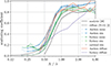 |
Figure 10. Random-incidence scattering coefficients for the 1D-sinusoidal surface, comparing different acquisition methods. The continuous lines represent the one-third octave averages of the corresponding dotted results. |
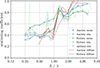 |
Figure 11. Random-incidence scattering coefficients for the 2D-rectangular surface, comparing different acquisition methods. The continuous lines represent the one-third octave averages of the corresponding dotted results. |
For the 1D-sinusoidal surface (Fig. 10), previous diffuse-field measurements of the same sample in a small-scale reverberation chamber (N = 5) [2] and analytical solutions were known from literature [34], which serves as a reference. Comparisons between free-field measurements and their simulations at both sites revealed an overestimation at lower frequencies, while difference converged towards eachother at higher frequencies. Comparing the numerical simulations between the Aachen and Sydney setups, a slight overestimation was observed for normalized frequencies Λ/λ ≤ 1; otherwise, the results were in good agreement. These deviations are attributed to differences in source and receiver geometries between the two setups, as the optimal simulation setup yield closer agreement to the analytical solution compared to the setup simulations. The diffuse-field measurements from literature are in the same range as the diffuse-field measurements in Aachen, where the diffuse-field measurements in Sydney are not. This can be attributed to the sample mounting, as it was not flush-mounted compared to the Aachen diffuse setup. In particular, the sinusoidal sample was not flush-mounted on the turntable, leaving an air gap. Finally, the comparison between diffuse-field measurements in Aachen and the free-field measurements showed that all results fall within the expected measurement uncertainty, as both methods exhibit similar deviations from the analytical solution.
For the 2D-rectangular surface (Fig. 11), previous measurements or analytical solutions were not available. All free-field results exhibit the typical “peaky” behavior associated with rectangular surface geometries before one-third octave averaging, known from [5]. At low normalized frequencies (Λ/λ < 1), the scattering coefficient appears to be significantly overestimated. This overestimation is likely due to pronounced edge effects, caused by multiple reflections at the surface edges [34]. These effects are more prominent for the 2D-rectangular structure due to its larger structural depth (5 cm), in contrast to the 1D-sinusoidal surface (2.04 cm). In the diffuse-field measurements, this edge effect is also present on both measurement sides. At higher frequencies (Λ/λ ≥ 1), both diffuse-field measurements show good agreement with the free-field results. Except for one diffuse-field measurement in Aachen and the measurement in Sydney, where the scattering coefficient exceeds 1 at higher frequencies. This behavior can likely be attributed to temperature fluctuations during the measurements. The temperature variation was approximately 2.2 ° C in Sydney and 0.7 ° C in Aachen, whereas for the measurements that did not exceed unity, the temperature fluctuation remained below 0.22 ° C. This observation is consistent with the findings of Vorländer et al. [2], who showed that time-varying environmental conditions, particularly temperature and humidity fluctuations, can introduce significant errors in reverberation-based measurements and lead to overestimated scattering coefficients. Repeated free-field measurements for both control surfaces showed good agreement in Aachen and Sydney, indicating reliable reproducibility.
5.2 Bidirectional scattering coefficients
The octave-band averaged bidirectional scattering coefficients (BSCs) for the 1D-sinusoidal and the 2D-rectangular surface are shown in Figures 12 and 13, respectively. The incident angle of 39° (relative to the surface’s normal) was selected as an example. Note that the measurement setups and the optimal simulation setup varies in incoming direction samplings, therefore the closest incoming direction was selected, which lead to a maximum difference of Δϑ = 1° between all setups.
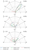 |
Figure 12. Bidirectional scattering coefficients (BSCs) for the 1D-sinusoidal surface for an incident angle of 39° ([mplRed] (0,0) circle (0.3mm);) for different octave frequency bands. |
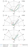 |
Figure 13. Bidirectional scattering coefficients (BSCs) for the 2D-rectangular surface for an incident angle of 39° ([mplRed] (0,0) circle (0.3mm);) for different octave frequency bands. |
The results are presented as a 2D polar cross-section. Since the incident wave is oriented perpendicular to the 1D surface corrugation, energy is confined to a single scattering plane [34] (compare with Fig. 15b).
The comparison of the 1D-sinusoidal surface (Fig. 12a) shows good agreement among all results for the specular reflection at 2 kHz. It should be noted that the optimal simulation result exhibits a slight shift, which can be attributed to the slightly different incident angle of 38°.
The comparison between the Sydney measurement and the corresponding simulation shows generally good agreement across all frequency bands. Figure 12c shows a reflection cone at 70° for the simulation but not for the measurement setup in Sydney, this can be explained by the very low SNR for large incident angles. Beside that the low SNR in the Sydney measurement does not significantly affect the results. When compared to the optimal setup, however, discrepancies become apparent at certain angles–most notably around 60° (Fig. 12b). This deviation is likely due to the limited angular resolution of the loudspeaker and receiver array, which may not accurately capture finer directional scattering features in that range, as this was captured by the simulation of the setup in Aachen. The retro-reflection at 4 kHz is present, even though it is underestimated by approximately 0.02 instead of 0.1, which might be attributed to the missing microphone position at the retro-reflective position.
The measurement in Aachen matches its simulation counterpart quite well for the specular reflection, except in the 4 kHz frequency band. The other reflection directions are well-aligned, with a slight underestimation for large incident angles and higher frequencies. This could be due to the lower SNR at these angles. The measurement setup simulation matches the optimal simulation quite well, with only slight underestimations for higher frequencies.
Compared to the 1D-sinusoidal surface, the 2D-rectangular surface results (Fig. 13) are more closely related. The results of the measurements and its numerical twins show good agreement for both measurement setups, except for slight underestimations at higher frequencies. These deviations are still within the expected measurement uncertainty of about ±0.1, which is similar to the difference between analytical solution and standard diffuse-field measurements as shown in Figure 12. Both measurement setups are also in good agreement with the optimal simulating setup, indicating reliable results.
6 Scattering behavior of different surface types
In the following, we present a selection of results for the overall database. All presented random-incidence coefficients are one-third octave band averaged frequency bands, while the bidirectional scattering coefficients are octave band averaged. This choice was made because the different band resolutions provide better visualization for each coefficient: one-third octave bands improve the spectral detail of random-incidence coefficients, while octave bands yield broader frequency band representation for bidirectional scattering coefficients. The frequency bands correspond to the measured frequency scale, unless stated otherwise.
6.1 Random surfaces
Figures 14 and 15 show the random-incidence and bidirectional scattering coefficients for randomly distributed hemispheres (coverage 50%), which was also measured in [39].
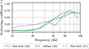 |
Figure 14. Random-incidence scattering coefficients for a randomly distributed hemispheres of radius 2 cm (coverage 50%) between optimal free-field simulation and diffuse-field measurement from [39]. |
Figure 14 demonstrates good agreement between the free-field simulation and the diffuse-field measurement data from [39], indicating that the proposed method is also applicable to randomly structured surfaces.
Furthermore, Figure 15 presents the BSCs for an incident angle of 39° at 8 kHz, as the scattering coefficients are almost similar for this frequency band. Surface 26 shows diffuse scattering characteristics, in contrast to the more directional scattering observed for the 1D periodic Surface 1. The simulation method successfully captures the extremely large differences in the sound reflection distribution, although the random-incidence scattering coefficients are rather similar. However, the measurement approach would require a higher SNR to resolve such low-level diffuse scattering contributions accurately.
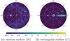 |
Figure 15. Bidirectional scattering coefficients for a random surface (a) and a periodic surface (b) obtained from free-field measurements at 8 kHz octave band. Incident direction is marked with red dot, while the cross marks the specular reflection. |
Figure 16 shows the directional scattering coefficient for each incident angle (ϑi), averaged over all azimuth angles (φi), derived from the optimal free-field simulation. Large variations between incident directions are observed, with values ranging approximately from 0.2 to 0.9, for example at 4 kHz. This indicates that the scattering behavior of the random surface strongly depends on the incident angle, because larger incident angles lead to greater effective roughness and therefore higher scattering. Consequently, the reflection behavior of random surfaces cannot be adequately described by the random-incidence scattering coefficients alone.
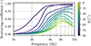 |
Figure 16. Directional scattering coefficients averaged over all azimuth angles (φ i ) for a random surface obtained from optimal free-field simulations. |
6.2 Modular surfaces
Figure 17 shows the random-incidence scattering coefficients and the three modular surfaces (6–8). It shows a good agreement between the free-field and diffuse-field measurements. Comparing Surface 6 and 7, which represent the same sample under different configurations, the additional elements lead to a significant increase in the scattering coefficient, particularly at lower frequencies. Similar to the rectangular diffuse field measurement in Figure 11 in Section 5.1, the diffuse field results exceed 1 for frequencies above 10 kHz. This is likely due to the temperature fluctuations between the measurement conditions of more than 1.45 ° C for both diffuse-field measurements.
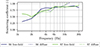 |
Figure 17. RSC for modular surfaces (S6 & S8) obtained from free-field and diffuse-field measurements in Sydney. |
6.3 Non-rigid surfaces
Figure 18 shows the random-incidence scattering coefficients and the absorption coefficients for the non-rigid Surfaces 9–12. ISO 17497-1:2004 [3] suggests an absorption coefficient below 0.5. Only Surface 10 satisfies this criterion, due to its polystyrene with an additional clay layer. Surface 12 satisfies this condition only at lower frequencies, likely because the surface is not entirely covered by polystyrene but also includes the wood of the baseplate. The remaining samples exhibit higher absorption because they consist entirely of polystyrene foam. The absorption coefficient may be overestimated due to the exposed sides of the sample in the reverberation-room measurements.
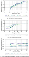 |
Figure 18. Random-incidence scattering coefficients and absorption coefficients for non-rigid surfaces. |
Surfaces 9 and 11 exhibit scattering coefficients greater than 1 above 1 kHz, whereas Surfaces 10 and 12 exceed 1 only at higher frequencies (8–10 kHz). This is likely caused by the high absorption of the samples, which reduces accuracy and also leads to a lower SNR in the measurements and therefore to increased uncertainty. In addition, the high temperature fluctuations within the measurement conditions for the 4 measurements are larger than 0.85 ° C, which might also contribute to the overestimation of the scattering coefficient.
For the free-field measurements, the lower SNR is more critical compared to the diffuse-field measurements. Surface 9, 11 and 12 show a good agreement between the free-field and diffuse-field measurements, until the diffuse-field measurement exceeds 1.
Due to a lack of numerical simulations or analytical solutions, the true scattering behavior of these surfaces remains unknown and the free-field measurements could not be validated.
6.4 Rectangular surface
Figure 19 shows the random-incidence scattering coefficients, comparing the free-field simulation with the analytical solution based on Embrechts and Billon [35].
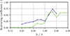 |
Figure 19. Random-incidence scattering coefficients for the 1D-rectangular surface (Surface 21) based on the optimal free-field simulation ([-,viridis2,solid,line width = 1.2pt](0,0) – (3mm,0);) and the analytical solution [35] ([-,viridis8,solid,line width = 1.2pt](0,0) – (3mm,0);). |
For Λ/λ ≥ 1, the results are in good agreement, while for lower values, differences of up to Δs = 0.2 are observed. This can be attributed to the finite size of the sample in the free-field simulation, compared to the infinite surface extent assumed in the analytical solution [35]. Therefore, the method was further validated through comparison with the analytical solution for an angular surface.
6.5 Facade surfaces
Figure 20 shows the random-incidence scattering coefficients for the facade in real frequency scale derived by Tokac et al. [10, 37]. Surface 16 and 18 were selected to represent the cladding and the division scale defined by [10], respectively. The differences between the free-field measurements and simulations are within the expected uncertainty range. The free-field measurements overestimate the scattering coefficient slightly.
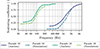 |
Figure 20. RSCs for facade surfaces in real scale from reduced scale free-field simulations (optimal) and measurements in Aachen. |
Figure 21 shows the random-incidence scattering coefficients for the other facades in real scale from free-field simulations (Surfaces 22–24). They are all within the same frequency range, since they all operate in the bay division scale.
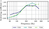 |
Figure 21. RSCs for additional facade surfaces in real scale obtained from free-field simulations. |
Figure 22 shows that, although the random-incidence scattering coefficients are relatively similar, the BSCs at an incident angle of 30° differs significantly. First, the scattering coefficients in the higher octave bands vary due to differences in the amount of energy directed into the specular reflection. Second, the redistribution of energy into non-specular directions differs markedly between the surfaces.
 |
Figure 22. One-third-octave band-averaged bidirectional scattering coefficients for two facade surfaces (Surfaces 22 and 24) obtained from free-field simulations and shown in octave bands for an incident angle of 30° ([mplRed] (0,0) circle (0.3mm);). |
6.6 Retroreflective surfaces
Similar to the scattering coefficient discussing the energy ratio into specular direction, other directions can be evaluated as well. In this case, the retroreflected energy derived from the BSC at an incident angle of 45° is shown in Figure 23 for a selection of surfaces.
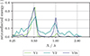 |
Figure 23. Retroreflected energy as a function of normalized frequency Λ/λ at an incident angle of approximately ϑ i ≈ 45° for a selection of surfaces obtained from free-field simulations. |
The retroreflective façade (Surface 24) exhibits the highest degree of retroreflection, followed by the sinusoidal surface (Surface 1). These results are consistent with the findings of Cabrera et al. [7], who also identified this type of geometry as retroreflective.
These results demonstrate that specific acoustic metrics, such as retroreflected energy, can be derived from the BSC to quantify particular scattering characteristics. This enables a more detailed analysis of directional reflection behavior than is possible using the RSC alone.
6.7 Singular objects
In acoustical terms, singular objects do not constitute a subset of a larger surface, as is the case with regular structures. Instead, their scattering behavior is unique to the specific object and its dimensions, rather than representing an extended surface. Although a scaling factor can still be applied, it must account not only for frequency and geometry but also for the object’s overall size.
Surfaces 14 and 15 are a spherical cap and a spiral-based vortex diffuser [40], respectively. The spherical cap is designed to focus sound, while the spiral is intended to scatter sound in multiple directions apart from the incident direction.
Figure 24 shows the BSCs for the singular objects at 16 kHz for 0.4778 m2. The spiral (Surface 15) scatters sound in multiple directions, with a notable reflection from reflection angles from 30° to 60°. These results confirm the intended acoustic functionalities of acoustic spiral.
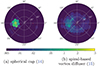 |
Figure 24. Bidirectional scattering coefficients for singular objects obtained from free-field measurements in the 16 kHz octave band for an effective area of 0.4778 m2. The incident direction is marked by a red dot, and the cross marks the specular reflection. |
The spherical cap (Surface 14) was designed to focus sound toward the dome’s transducers in the Sydney measurement setup. As a result, the transducers are not located in the far field. However, this method can still capture near-field scattering behavior, similar to the way diffusion coefficients do [20]. The current results seem plausible; nonetheless, validation with respect to analytical solution formulations (e.g., [41]) lies outside the present scope.
6.8 Compilation of the results into a database
To enable practical use of directional scattering information, the measured bidirectional scattering coefficients were compiled into a structured database [33]. Providing access to the directional data allows measured surface properties to be incorporated directly into sound propagation models and avoids the need to approximate complex surfaces by simplified scattering parameters.
The database stores the bidirectional scattering coefficient together with the corresponding measurement and surface metadata. This includes information on geometry, measurement conditions, and frequency resolution, enabling reproducibility and facilitating further numerical or experimental studies. In addition, the database contains the RSC derived from the BSC as well as the diffuse-field measured RSC. All data are provided in the SOFA format [42], allowing standardized exchange and direct implementation in existing acoustical simulation frameworks. Table 1 provides an overview of the surfaces included in the database, which comprises 29 different geometries.
Properties of all surfaces in the database including the control surfaces (0–2) and the extension (3–28).
The database includes the raw measurement data, raw simulation results, and the complete processing workflow [43] required to reproduce the reported scattering coefficients. Providing these components enables independent verification and ensures transparency of the data processing.
7 Discussion and conclusion
A broad range of different surfaces was measured and simulated, covering periodic, random and non-rigid surfaces, as well as singular objects. A couple of real facades were also included in the analysis, covering a range of architectural scales, such as bay division and cladding elements [10]. The 1D sinusoidal and the 2D rectangular surface served as control surfaces and were measured in Aachen and in Sydney and were simulated numerically. For the 1D sinusoidal previous diffuse-field measurements and analytical solutions served as a reference.
The free-field method demonstrates reliability for a variety of introduced surface types. Randomly structured surfaces, such as randomly distributed hemispheres, also yield reliable results. The method was able to capture the diffuse reflection characteristics of these surfaces, as demonstrated by the BSCs. It was shown that the directional scattering coefficient varies for different incidence angles, therefore, the reflection behavior of random surfaces cannot be adequately described by the random-incidence scattering coefficients alone.
Surfaces made of different variations of polystyrene and clay demonstrated the limitations of the measurement method. The diffuse-field method resulted in scattering coefficients larger than 1, so a comparison could not be made. Due to a lack of known coefficients the free-field method could also not be validated for this surfaces. The low SNR might lead to unreliable results. Further simulations on sound-reflecting and absorptive materials of known surfaces – e.g. sinusoidal or rectangular – with artificial noise could help determine the minimum required SNR for a given error threshold.
The analysis also includes 1D retro-reflective surfaces, such as a standard 1D-triangular profile (Surface 20) and the façade of the Ainsworth Building (Surface 24) in Sydney [7], which also features a 1D-triangular geometry coupled with perpendicular bars. It has been demonstrated that specific acoustic metrics, such as retro-reflected energy, can be derived from the bidirectional scattering coefficients (BSCs).
The analysis also includes singular objects, for which the BSC is valid only for the specific object and its exact dimensions. The results demonstrated plausible scattering behavior, confirming the intended acoustic functionality of these objects. This indicates that the free-field method is suitable for characterizing singular objects as well.
The inter-laboratory comparison of 1D-sinusoidal control surfaces between Aachen and Sydney shows a high degree of consistency in both random-incidence scattering coefficients and BSCs, where the 2D-rectangular control surface shows less consistency in the results.
One factor is the edge effect, which is more dominant for the 2D-rectangular surfaces than for the 1D-sinusoidal surface. The reason is that for the correlation method, the edge effect is compensated best if the edges of the flat reference surface and the rectangular surface are at the same physical position. Therefore the positioning of the sample is very critical, depending on the surface properties. For the 1D-sinusoidal surface, the effect is reduced, due to the changing height along the edge. For the 2D-rectangular surface, the edge effect is more pronounced, as the edges are either at the surface minimum or maximum depth. It was also previously shown that 1D-rectangular surfaces lead to larger derivations to analytical reference than sinusoidal surfaces with accurate positioning and equal height-to-structural wavelength ratios [44]. The comparison to the analytic reference of rectangular surfaces is also less consistent compared to sinusoidal surfaces.
The edge effect influence needs to be studied in more detail, especially for the angular surfaces. Additionally, the larger height-to-structural wavelength ratio of the 2D-rectangular surface (h/Λ = 0.67) compared to the 1D-sinusoidal surface (h/Λ = 0.29) leads to a more pronounced edge effect.
The inter-laboratory comparison showed that retro-reflections were significantly underestimated in the BSC based on the Sydney measurement and its simulation for both control surfaces, as the loudspeaker was active at this time, leading to a gap in the receiver array at the retro-reflection angle.
The Sydney measurement geometry showed also some limitations, due to the limited resolution of the loudspeaker array. Additionally, lots of loudspeakers are on the ground plane. This results in higher errors due to the more difficult windowing. Therefore, the Sydney measurement setup could be optimized by relocating the 30 loudspeakers from the lower plane (φ s = 90°) and increasing the array density below φ s = 70°.
A key observation is that signal-to-noise ratios (SNRs) were generally lower than the 40 dB recommended in [20], with both laboratories operating below this threshold. Despite the SNRs being below the recommended threshold, the consistency in the control surfaces suggests that the measurement procedure is robust. Nevertheless, it is very interesting that the reciprocal approach applied to the loudspeaker array worked out quite well. With this it could be demonstrated that hemispherical receiver grids are useful as such, however, with careful consideration of the geometrical distribution of the receivers.
Furthermore, the results were compiled into an open dataset, which offers a standardized and comprehensive collection of acoustic scattering data, stored in the SOFA format [42], and enriched with detailed metadata describing the surfaces, measurement or simulation setups, and results. The dataset is openly available under a CC-BY 4.0 license via Zenodo [33], ensuring accessibility and transparency. Its modular design also allows for straightforward future extensions by the research community.
Acknowledgments
The authors would like to thank Florian Braun for conducting the diffuse-field measurements in Aachen, and Anthony Donoghue for assistance with fabrication of samples in Sydney. Computations were performed with computing resources granted by RWTH Aachen University under project rwth1245.
Funding
This work was funded by the Deutsche Forschungsgemeinschaft (DFG, German Research Foundation) under the project number https://gepris.dfg.de/gepris/projekt/456072683, and by the Australian Government through the Australian Research Council’s Discovery Projects funding scheme (project DP230101357).
Conflicts of interest
The authors declare no conflict of interest.
Data availability statement
The research data associated with this article are available in Zenodo, under the reference [33]. The code for this article is available in Zenodo, under the reference [43].
References
- T. Cox, P. d’Antonio: Acoustic Absorbers and Diffusers: Theory, Design and Application, 3rd edn. CRC Press, 2016. [Google Scholar]
- M. Vorländer, J.-J. Embrechts, L.D. Geetere, G. Vermeir: Case studies in measurement of random incidence scattering coefficients. Acta Acustica United with Acustica 90 (2004) 858–867. [Google Scholar]
- ISO 17497-1:2004: Sound-Scattering Properties of Surfaces. Part 1: Measurement of the Random-Incidence Scattering Coefficient in a Reverberation Room. International Organization for Standards, Geneva, Switzerland, 2004. [Google Scholar]
- M. Vorländer: Auralization: Fundamentals of Acoustics, Modelling, Simulation, Algorithms and Acoustic Virtual Reality. RWTHedition. Springer International Publishing, Cham, 2020. ISBN 978-3-030-51201-9 978-3-030-51202-6. [Google Scholar]
- M. Vorländer, S. Feistel: Show your scattering coefficients, in: Proceedings of Meetings on Acoustics. Vol. 50, 2024, pp. 015003. URL https://doi.org/10.1121/2.0001816. [Google Scholar]
- J.W.S.B. Rayleigh: The Theory of Sound, 2nd edn. Vol. 11. Dover Publications, Macmillan, New York, 1896. [Google Scholar]
- D. Cabrera, M. Yadav, J. Holmes, O. Fong, H. Caldwell: Incidental acoustic retroreflection from building façades: three instances in Berkeley, Sydney and Hong Kong. Building and Environment 172 (2020) 106733. ISSN 0360-1323. [Google Scholar]
- J. Kang: Sound propagation in street canyons: comparison between diffusely and geometrically reflecting boundaries. The Journal of the Acoustical Society of America 107, 3 (2000) 1394–1404. ISSN 0001-4966, 1520-8524. [Google Scholar]
- J. Picaut, L. Simon: A scale model experiment for the study of sound propagation in urban areas. Applied Acoustics 62, 3 (2001) 327–340. ISSN 0003-682X. [Google Scholar]
- I. Tokac, A. Heimes, M. Vorländer, S. Brell-Cokcan: A rule-based framework for capturing geometric characteristics in design: a study of façade analysis for acoustic behaviour in urban space. International Journal of Architectural Computing 23, 2 (2025) 405–425. ISSN 1478-0771. [Google Scholar]
- F.E. Nicodemus, J.C. Richmond, J.J. Hsia, I.W. Ginsberg, T. Limperis: Geometrical Considerations and Nomenclature for Reflectance. Vol. 160. US Department of Commerce, National Bureau of Standards Washington, DC, USA, 1977. [Google Scholar]
- S. Siltanen, T. Lokki, S. Kiminki, L. Savioja: The room acoustic rendering equation. The Journal of the Acoustical Society of America 122, 3 (2007) 1624–1635. [Google Scholar]
- W. Binek, A. Pilch, T. Kamisiński: Direct application of the diffusers’ reflection patterns in geometrical acoustics simulations. Applied Acoustics 198 (2022) 108949. ISSN 0003-682X. [Google Scholar]
- J.A. Hargreaves: Acquisition of bi-directional reflectance functions by Nearfield Acoustical Holography – a preliminary study, 2019. URL https://salford-repository.worktribe.com/output/1366577. [Google Scholar]
- E. Brandão, E. Fernandez-Grande, C. Gaudeoso, S.A. Verburg, A. Richard: Three-dimensional directivity measurement of acoustic diffusers using regularized holography and sound field separation. The Journal of the Acoustical Society of America 158, 5 (2025) 3936–3948. ISSN 0001-4966. [Google Scholar]
- A. Heimes, M. Vorländer: Bidirectional surface scattering coefficients. Acta Acustica 9 (2025) 41. ISSN 2681-4617. [Google Scholar]
- D. Cabrera, L. Miranda, D. Jimenez, C. Edser, W.L. Martens: A facility for simulating room acoustics, employing a high density hemispherical array of loudspeakers. Acoustics Australia 43, 1 (2015) 77–81. ISSN 1839-2571. [Google Scholar]
- J.-G. Richter, G. Behler, J. Fels: Evaluation of a fast HRTF measurement system, in: Audio Engineering Society Convention. Vol. 140. Audio Engineering Society, 2016. [Google Scholar]
- P. Majdak, P. Balazs, B. Laback: Multiple exponential sweep method for fast measurement of head-related transfer functions. Journal of the Audio Engineering Society 55, 7/8 (2007) 623–637. [Google Scholar]
- ISO 17497-2:2012: Sound-Scattering Properties of Surfaces. Part 2: Measurement of the Directional Diffusion Coefficient in a Free Field. International Organization for Standards, Geneva, Switzerland, 2012. [Google Scholar]
- V.E. Ostashev, D.K. Wilson: Acoustics in Moving Inhomogeneous Media, 2nd edn. CRC Press, London, 2015. ISBN 978-0-429-17649-4. [Google Scholar]
- A. Heimes: mesh2scattering version: 1.0.0 (Python 3.10), 2025. URL https://github.com/ahms5/Mesh2scattering. [Google Scholar]
- F. Brinkmann, W. Kreuzer, J. Thomsen, S. Dombrovskis, K. Pollack, S. Weinzierl, P. Majdak: Recent advances in an open software for numerical HRTF calculation. Journal of the Audio Engineering Society 71, 7/8 (2023) 502–514. [Google Scholar]
- W. Kreuzer, K. Pollack, F. Brinkmann, P. Majdak: NumCalc: an open-source BEM code for solving acoustic scattering problems. Engineering Analysis with Boundary Elements 161 (2024) 157–178. ISSN 0955-7997. [Google Scholar]
- D.T. Bradley, M. Müller-Trapet, J. Adelgren, M. Vorländer: Effect of boundary diffusers in a reverberation chamber: standardized diffuse field quantifiers. The Journal of the Acoustical Society of America 135, 4 (2014) 1898–1906. ISSN 0001-4966. [Google Scholar]
- pyfar-developers: Pyfar version: 0.6.8 (Python 3.10), 2024. [Google Scholar]
- pyfar-developers: Pyrato version: 0.4.2 (Python 3.10), 2024. [Google Scholar]
- W.T. Chu: Comparison of reverberation measurements using Schroeder’s impulse method and decay-curve averaging method. The Journal of the Acoustical Society of America 63, 5 (1978) 1444–1450. ISSN 0001-4966. [Google Scholar]
- A. Lundeby, T.E. Vigran, H. Bietz, M. Vorländer: Uncertainties of measurements in room acoustics. Acustica 81 (1995) 344–355. [Google Scholar]
- M. Guski, M. Vorländer: Comparison of noise compensation methods for room acoustic impulse response evaluations. Acta Acustica United with Acustica 100, 2 (2014) 320–327. ISSN 16101928. [Google Scholar]
- ISO 3382: Acoustics – Measurement of the Reverberation Time of Rooms with Reference to Other Acoustical Parameters. International Organization for Standards, Geneva, Switzerland, 2004. [Google Scholar]
- ISO 9613-1:1993: Acoustics – Attenuation of Sound During Propagation Outdoors – Part 1: Calculation of the Absorption of Sound by the Atmosphere. International Organization for Standards, Geneva, Switzerland, 1993. [Google Scholar]
- A. Heimes, D. Cabrera, D. Reinhardt, I.T. Celikyay, S. Brell-Cokcan, M. Vorländer: Database of acoustic bidirectional and random-incidence scattering coefficients, 2025. URL https://doi.org/10.5281/zenodo.17660108. [Google Scholar]
- J.-J. Embrechts, L.D. Geetere, G. Vermeir, M. Vorländer, T. Sakuma: Calculation of the random-incidence scattering coefficients of a sine-shaped surface. Acta Acustica United with Acustica 92 (2006) 593–603. [Google Scholar]
- J.-J. Embrechts, A. Billon: Theoretical determination of the random-incidence scattering coefficients of infinite rigid surfaces with a periodic rectangular roughness profile. Acta Acustica United with Acustica 97, 4 (2011) 607–617. [Google Scholar]
- L. Aspöck, F. Brinkmann, D. Ackermann, S. Weinzierl, M. Vorländer: BRAS – Benchmark for room acoustical simulation, 2020. URL https://doi.org/10.14279/depositonce-6726.3. [Google Scholar]
- I. Tokac, H. Knitt, A. Heimes, M. Vorlaender, S. Brell-Cokcan: Rule-based automation for combining design and robotic fabrication: a case study on acoustic evaluation of building facades using robotically milled physical models, 2025. URL https://papers.ssrn.com/abstract=5110206. [Google Scholar]
- J. Llorca-Bofí, C. Dreier, J. Heck, J. Kempin, M. Vorländer: IHTApark. Multi-detailed 3D architectural model for sound perception research in virtual reality, 2022. URL https://doi.org/10.5281/zenodo.5905338. [Google Scholar]
- M.H. de Avelar Gomes, M. Vorländer, S.N.Y. Gerges: Anforderungen an die Probeflachengeometrie bei der Messung des Streugrades im Diffusfeld. Fortschritte der Akustik 28 (2002) 584–585. [Google Scholar]
- N. Jiménez, J.-P. Groby, V. Romero-García: Vortex-sound diffusers using spiral metasurfaces, in: 2018 12th International Congress on Artificial Materials for Novel Wave Phenomena (Metamaterials), 2018, pp. 194–196. URL https://doi.org/10.1109/MetaMaterials.2018.8534047. [Google Scholar]
- M. Vercammen: Sound concentration caused by curved surfaces. Ph.D. thesis, Eindhoven University of Technology, 2012. [Google Scholar]
- AES Standards Committee: AES69-2022: AES standard for file exchange – Spatial acoustic data file format, 2022. URL https://www.aes.org/publications/standards/search.cfm?docID=99. [Google Scholar]
- A. Heimes, D. Cabrera, D. Reinhardt, I.T. Celikyay, S. Brell-Cokcan, M. Vorländer: Workflow for the paper ‘Interlaboratory Comparison and Analysis of Bidirectional Scattering Coefficients for Various Surfaces’, 2025. URL https://doi.org/10.5281/zenodo.17700694. [Google Scholar]
- A. Heimes, L. Pan, M. Vorländer: Numerical simulation and analysis of surface scattering – Part 1, in: Forum Acusticum 2023, Torino, Italy, 2023. [Google Scholar]
Cite this article as: Heimes A. Cabrera D. Holmes J. Reinhardt D. Tokac Celikyay I. Brell-Cokcan S. & Vorländer M. 2026. Interlaboratory Comparison and Analysis of Bidirectional Scattering Coeffcients for Various Surfaces. Acta Acustica, 10, 65. https://doi.org/10.1051/aacus/2026060.
All Tables
Properties of all surfaces in the database including the control surfaces (0–2) and the extension (3–28).
All Figures
|
Figure 1. Measurement setup in Aachen, Germany. |
| In the text | |
|
Figure 2. SNR for the first (top) and second (bottom) measurement series in Aachen. |
| In the text | |
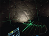 |
Figure 3. Measurement setup in Sydney, Australia [17]. |
| In the text | |
|
Figure 4. Hardware setup for a single channel of the reciprocal measurement system used in Sydney. |
| In the text | |
|
Figure 5. SNR for the measurement series in Sydney. |
| In the text | |
|
Figure 6. All geometrical setups with the sample ([-,mplBlue,solid,line width = 0.9pt](0,0) – (3mm,0);). (a) The measurement setup in Aachen with loudspeaker positions ([-,mplRed,solid,line width = 0.9pt](0,0) – (3mm,0);) and the microphone arc ([-,mplGreen,solid,line width = 0.9pt,opacity=0.8](0,0) – (3mm,0);) resulting in a total receiver array ([-,mplGreen,solid,line width = 0.9pt,opacity=0.4](0,0) – (3mm,0);) after the measurement procedure. (b) The measurement setup in Sydney with loudspeaker positions ([-,mplRed,solid,line width = 0.9pt](0,0) – (3mm,0);). (c) The optimal far-field simulation setup with the incidence plane waves in ([-,mplRed,solid,line width = 0.9pt](0,0) – (3mm,0);) and the receiver positions ([-,mplGreen,solid,line width = 0.9pt,opacity=0.8](0,0) – (3mm,0);). |
| In the text | |
|
Figure 7. Small-scale reverberation room in Aachen, Germany. |
| In the text | |
|
Figure 8. Small-scale reverberation chamber in Sydney, Australia. |
| In the text | |
|
Figure 9. Sample identifiers and images of the selected surfaces, with singular objects highlighted with *. Large images are available in the dataset [33]. |
| In the text | |
|
Figure 10. Random-incidence scattering coefficients for the 1D-sinusoidal surface, comparing different acquisition methods. The continuous lines represent the one-third octave averages of the corresponding dotted results. |
| In the text | |
|
Figure 11. Random-incidence scattering coefficients for the 2D-rectangular surface, comparing different acquisition methods. The continuous lines represent the one-third octave averages of the corresponding dotted results. |
| In the text | |
|
Figure 12. Bidirectional scattering coefficients (BSCs) for the 1D-sinusoidal surface for an incident angle of 39° ([mplRed] (0,0) circle (0.3mm);) for different octave frequency bands. |
| In the text | |
|
Figure 13. Bidirectional scattering coefficients (BSCs) for the 2D-rectangular surface for an incident angle of 39° ([mplRed] (0,0) circle (0.3mm);) for different octave frequency bands. |
| In the text | |
|
Figure 14. Random-incidence scattering coefficients for a randomly distributed hemispheres of radius 2 cm (coverage 50%) between optimal free-field simulation and diffuse-field measurement from [39]. |
| In the text | |
|
Figure 15. Bidirectional scattering coefficients for a random surface (a) and a periodic surface (b) obtained from free-field measurements at 8 kHz octave band. Incident direction is marked with red dot, while the cross marks the specular reflection. |
| In the text | |
|
Figure 16. Directional scattering coefficients averaged over all azimuth angles (φ i ) for a random surface obtained from optimal free-field simulations. |
| In the text | |
|
Figure 17. RSC for modular surfaces (S6 & S8) obtained from free-field and diffuse-field measurements in Sydney. |
| In the text | |
|
Figure 18. Random-incidence scattering coefficients and absorption coefficients for non-rigid surfaces. |
| In the text | |
|
Figure 19. Random-incidence scattering coefficients for the 1D-rectangular surface (Surface 21) based on the optimal free-field simulation ([-,viridis2,solid,line width = 1.2pt](0,0) – (3mm,0);) and the analytical solution [35] ([-,viridis8,solid,line width = 1.2pt](0,0) – (3mm,0);). |
| In the text | |
|
Figure 20. RSCs for facade surfaces in real scale from reduced scale free-field simulations (optimal) and measurements in Aachen. |
| In the text | |
|
Figure 21. RSCs for additional facade surfaces in real scale obtained from free-field simulations. |
| In the text | |
|
Figure 22. One-third-octave band-averaged bidirectional scattering coefficients for two facade surfaces (Surfaces 22 and 24) obtained from free-field simulations and shown in octave bands for an incident angle of 30° ([mplRed] (0,0) circle (0.3mm);). |
| In the text | |
|
Figure 23. Retroreflected energy as a function of normalized frequency Λ/λ at an incident angle of approximately ϑ i ≈ 45° for a selection of surfaces obtained from free-field simulations. |
| In the text | |
|
Figure 24. Bidirectional scattering coefficients for singular objects obtained from free-field measurements in the 16 kHz octave band for an effective area of 0.4778 m2. The incident direction is marked by a red dot, and the cross marks the specular reflection. |
| In the text | |
Current usage metrics show cumulative count of Article Views (full-text article views including HTML views, PDF and ePub downloads, according to the available data) and Abstracts Views on Vision4Press platform.
Data correspond to usage on the plateform after 2015. The current usage metrics is available 48-96 hours after online publication and is updated daily on week days.
Initial download of the metrics may take a while.