| Issue |
Acta Acust.
Volume 10, 2026
|
|
|---|---|---|
| Article Number | 25 | |
| Number of page(s) | 17 | |
| Section | General Linear Acoustics | |
| DOI | https://doi.org/10.1051/aacus/2026017 | |
| Published online | 09 April 2026 | |
Scientific Article
Automated Sound Field Estimation combining robotized acoustic measurements and the boundary elements method
1
LMI, ENSTA, Institut Polytechnique de Paris, 828 Boulevard des Maréchaux, 91120 Palaiseau, France
2
U2IS, ENSTA, Institut Polytechnique de Paris, 828 Boulevard des Maréchaux, 91120 Palaiseau, France
3
POEMS, CNRS, Inria, ENSTA, Institut Polytechnique de Paris, 91120 Palaiseau, France
* Corresponding author: This email address is being protected from spambots. You need JavaScript enabled to view it.
Received:
9
October
2025
Accepted:
11
February
2026
Abstract
The identification and reconstruction of acoustic fields radiated by unknown structures is usually performed using either Sound Field Estimation or Near-field Acoustic Holography techniques. The latter turns out to be especially useful when data is only available close to the source, but information throughout the whole space is needed. Yet, the lack of amendable and efficient implementations of state-of-the-art solutions, as well as the laborious and often lengthy deployment of acoustic measurements continue to be significant obstacles to the practical application of such methods. The purpose of this work is to address both problems. First, a completely automated metrology setup is proposed, in which a robotic arm is used to gather extensive and accurately positioned acoustic data without any human intervention. The impact of the robot on acoustic pressure measurements is cautiously evaluated, and proved to remain limited below 1 kHz. The Sound Field Estimation is then tackled using the Boundary Element Method, and implemented using the FreeFEM software. Numerically simulated measurements have allowed us to assess the method accuracy, which matches theoretically expected results and proves to remain robust against positioning inaccuracies, provided that the robot is carefully calibrated. The overall solution has been successfully tested using actual robotized measurements of an unknown loudspeaker, with a reconstruction error of less than 30%.
Key words: Sound Field Estimation / Boundary Elements Method / Robotized acoustic metrology
© The Author(s), Published by EDP Sciences, 2026
 This is an Open Access article distributed under the terms of the Creative Commons Attribution License (https://creativecommons.org/licenses/by/4.0), which permits unrestricted use, distribution, and reproduction in any medium, provided the original work is properly cited.
1 Introduction
The reconstruction of the acoustic pressure field radiated by an arbitrary source, using only a limited set of actual microphone measurements, is a common task in experimental acoustics. In particular, Sound Field Estimation (SFE) aims at accurately predicting the far-field properties of a studied source based on near-field measurements. In that way, it is possible to study the impact of the source in its environment, without having to perform wide range measurements at a large distance from the source. This method has proven to be relevant for loudspeaker characterization [1], but also for the study of other noise sources, such as aircraft [2], UAVs [3], cars [4] or daily life items [5]. On the other hand, Near-field Acoustic Holography (NAH) objective is to estimate the surfacic acoustic features of a radiating source using near-field measurements. Unlike SFE, NAH has to solve an inverse problem, and requires an additional regularization step. Yet, NAH algorithms may also be used to solve SFE problems [6, 7], and will equivalently be considered in the following.
The foundations of SFE and NAH rely on two main aspects: the practical acoustic measurements and the reconstruction method.
1.1 Acoustic measurements
One of the main challenges encountered while performing SFE acoustic measurements is the need to perform numerous accurately positioned, near-field measurements.
This issue has been addressed by the use of microphone arrays, which consist of a rigid assembly of microphones, which fixed at a given distance from the source. Such arrays come in various geometries – linear [8], planar [9], cylindrical [10], spherical [3] – but often lack versatility. Their high cost makes it impractical to design a new array for each object under study. Additionally, the simultaneous operation of multiple microphones requires specialized hardware and careful calibration of the array [11].
To enable variable resolution and large-scale measurements, the concept of mobile arrays was quickly introduced: rigid arrays are mounted on one [12], two [13, 14] or three [15, 16] prismatic joints, or one revolute joint [17], and moved around the source to collect the required data. However, depending on the axes’ layout, some positions and orientations of the microphones remain unreachable.
Recent work have proposed to combine motion tracking [18], 2D [19] and 3D [20] localization methods with acoustic measurements, so that the microphone, or microphone array, is continuously located during the process. If such approaches lead to a greater versatility and the ability to perform measurements at a larger scale, they are still limited by occlusion issues, and does not enable fully autonomous measurements.
Eventually, the use of multiple Degrees of Freedom (DOF) robots for acoustic measurements has been considered, with for instance the robotized NAH solution proposed by Klippel [1], using a cylindrical robot with 3 DOF.
The use of full 6 DOF robots in acoustic however still remains scarce, with few applications in non-destructive testing [21, 22], room acoustics [23], and NAH [24, 25]. However, most of these procedures still limit themselves to planar measurements, and are not taking the full benefits of the maneuverability and autonomy of the robot. Furthermore, the actual impact of the robot on the measurements, both in terms of positioning accuracy [26] and acoustic footprint, remains to be assessed.
1.2 Sound field estimation
In its most generic form, SFE allows for a temporal as well as a spatial estimation of the sound field, that is, the sought acoustic quantity is expressed as a function of both space and time. In our case however, we will assume that the studied source is stationary, and that the sound field is only a function of space, with a harmonic time dependency.
As for most identification problems, SFE relies on two major steps: modeling and identification. The modeling step essentially translates the way the sound field is represented. Two options were mainly investigated in the literature: expansion-based methods, where the sound field is written as an expansion of elementary solutions, and discretization-based methods, where the sound field is found by solving Helmholtz equation over a discretized space.
Maynard and Williams [27] originally investigated the first approach, using a Spatial Fourier Transform (SFT) method. However, it lacks flexibility, as the elementary solutions are limited to a few simple separable geometries. It is also impacted by windowing and aliasing effects [13, 28].
The expansion approach has then been intensively investigated in order to cope with SFT issues. Statistically Optimized NAH (SONAH) method proposed by Hald [28], dealt with the frequency aliasing issue by considering a continuous approach of the wave-number space. Helmholtz Equation Least Squares (HELS) method proposed by Wu [4] opted for spheroidal elementary solutions as the expansion set. Equivalent Source Method (ESM) [29] proposed a more tangible modeling approach, using isolated and distributed [30] artificial sources as elementary solutions. In particular, the spherical harmonics expansion [1] uses punctual acoustic sources, defined by a finite sum of spherical harmonics, which allows for an accurate reconstruction of the sound field with a limited expansion set. However, in the end, all these methods require (i) a clever choice of expansion set [31, 32] and (ii) a discretization choice on this set to ensure a good trade-off between reconstruction accuracy, computational resources and the risk of over-fitting [30].
The identification of the expansion coefficients is often performed using a least-squares approach, combined with a regularization scheme to ensure the reconstruction regularity, especially when solving NAH problems [33, 34]. Recent developments, benefiting from the compressive sensing theory, have proposed a sparse identification of the expansion coefficients [35], in order to avoid the energy spreading effect caused by an L 2 norm minimization. A lower order norm minimization [36] indeed leads to a concentration of the energy on a few expansion functions, or artificial sources, hence allowing for a better reconstruction accuracy far from the measurements.
On the other hand, several works opted for a direct resolution of Helmholtz equation, resorting to geometric and algebraic discretization schemes. For instance, Finite Elements Method (FEM) [37] and Inverse Patch Transfer Functions (IPTF) [14, 16, 20] have been considered for this task, but respectively suffer from an impractical adaptation to SFE problems and increased measurement costs. In comparison, Boundary Elements Method (BEM) [5, 8, 18, 34, 38] provides an alternative suited for SFE infinite domains, and with reasonable practical needs, as the only requirement is that measurements are to be performed on the nodes of a surfacic mesh surrounding the studied source. Furthermore, unlike expansion-based methods, the impact of the chosen discrete function space can be predicted a priori, and the method is not impacted by frequential aliasing, or by the placement of artificial sources. However, such flexibility comes at a cost, as computations are inherently more complex, and resources consuming.
It should be noted that the recent emergence of learning-based methods in physics-based problems have led to the use of convolutional [39] and physics informed [40, 41] neural networks to solve SFE problems. Although these methods have shown promising results, they are still limited by the need of a large amount of data, and the lack of physical guarantees and interpretations of the results.
Despite their great diversity, all these methods still remain scarcely implemented, especially in open-source software, and often prove to be poorly coupled with the actual measurements step.
1.3 Problem statement and contributions
The practical setup of SFE tools is hindered by two major drawbacks: the lack of efficient implementation of the existing numerical methodologies, and the time-consuming and tedious roll-out of acoustic measurements. Therefore, we present a novel acoustic sound field estimation methodology, handling both the measurements and reconstruction steps. The measurements are performed using a 7 DOF arm robot, allowing for numerous and versatile measurements, and the reconstruction is performed using an optimized parallel implementation of BEM [42, 43]. Bearing in mind that the quality of a metrology system depends on the impact of each item in the acquisition chain, the actual impact of the robot on the measurements is assessed, and the underlying effects on the reconstructed sound field are discussed.
2 Boundary Elements Method for sound field estimation
In this section, we will focus on the resolution of the sound field estimation problem using BEM, with a particular emphasis on its theoretical performance and robustness against robot-induced measurement errors.
2.1 Previous work
The boundary elements method is a numerical method used to solve partial differential equations, that is particularly well suited for problems where a solution is sought over an infinite domain [44, 45]. The equations derived from BEM are solely defined on the boundary of the domain. Hence, the solution at any field point can be obtained with no need for a domain wide discretization.
This boundary-wise approach made BEM a perfect candidate for the resolution of Helmholtz equation in NAH [8, 34, 38, 46] and SFE problems [5, 18]. In the latter case, the practical use of BEM with a free-field hypothesis is often hindered by the required boundary conditions, which consist in a set of acoustic measurements performed on closed mesh surrounding the studied source. However, the use of robotized measurements should conveniently ensure the reachability of the targeted mesh nodes.
2.2 Problem derivation and resolution methodology
SFE problem can be formulated as an exterior Dirichlet problem for Helmholtz equation. We seek a solution of the free-field acoustic equation in the infinite 3D space, knowing its value on a bounded surface.
As pictured on Figure 1, let us denote by ∂Ω the surface on which the measurements are performed, and by Ω the exterior domain over which the complex sound field p is studied. Unlike SFT-based methods, no particular constraint is set on the shape of ∂Ω, but it must define a smooth closed surface around the studied source. In this situation, Helmholtz equation, for a constant wave number k ∈ ℝ, and under the harmonic hypothesis, is written as
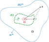 |
Figure 1. Dirichlet exterior problem for the Helmholtz equation. |
![Mathematical equation: $$ \begin{aligned} {\left\{ \begin{array}{ll} \mathrm{\Delta } p + k^2 p = 0&\text{ in} ~~ \mathrm{\Omega }, \\ [5pt] p = p_{0}&\text{ on} ~~ \partial \mathrm{\Omega }, \\ [5pt] \lim _{\partial \mathrm{\Omega }^{\infty } \rightarrow \infty } \left(\frac{\partial }{\partial |x|} - ik\right)p(x) = 0. \\ \end{array}\right.} \end{aligned} $$](/articles/aacus/full_html/2026/01/aacus250165/aacus250165-eq1.gif) (1)
(1)
The last condition on ∂Ω∞ is the Sommerfeld radiation condition, which ensures that the solution p behaves as a spherical wave at infinity, and is physically acceptable. It states that the sound field p should not grow faster than a spherical wave at infinity, and that it should not contain any component coming from the far field.
The free-space Green function (or fundamental solution) G associated to equation (1) is given by
 (2)
(2)
and allows to define a so-called combined potential C as [44]
 (3)
(3)
with u regular enough to be integrated on ∂Ω and dσ defining the surface measure on ∂Ω.
The boundary elements method is then built on the proof that this potential is an infinitely differentiable solution of equation (1) on Ω \ ∂Ω, stable for all wavenumbers k. The only requirement to extend it over all Ω consists in finding a boundary density u on ∂Ω such that the boundary conditions are satisfied.
Introducing the Dirichlet trace operator γ 0 ∂Ω, which extends on ∂Ω sufficiently smooth functions defined on Ω \ ∂Ω, this problems can be written as
![Mathematical equation: $$ \begin{aligned} \begin{aligned}&\exists ~u: \partial \mathrm{\Omega } \rightarrow \mathbb{C} , ~ \gamma _0^{\partial \mathrm{\Omega }} \left[C(u)\right] \\&\qquad = \frac{u}{2} + K(u) - ik V(u) = p_{0}, \end{aligned} \end{aligned} $$](/articles/aacus/full_html/2026/01/aacus250165/aacus250165-eq4.gif) (4)
(4)
where V and K denote the Boundary Integral Operators (BIOs) arising from the Dirichlet traces of two surfacic integrals on ∂Ω.
Both BIOs contain singular surfacic integrals, involving the ill-defined evaluation of the free-space Green function on ∂Ω. Yet, their calculations are still possible but require u S and u D to belong in a particular space of functions with sufficient regularity guarantees, and significant computational efforts (e.g. specific quadrature formulas for singular integrals computation).
Eventually, equation (4) defines a Boundary Integral Equations (BIE), which can be solved using a Galerkin approximation, where u is sought in a finite dimensional subspace V h
![Mathematical equation: $$ \begin{aligned} \begin{aligned}&\exists ~u \in V_h, \forall v \in V_h, \\&\int _{\partial \mathrm{\Omega } \times \partial \mathrm{\Omega }} \left[\frac{u(y)}{2} + K(u)(y) - ikV(u)(y)\right]v(x)\,\mathrm{d}\sigma (x,y) \\&\qquad = \int _{\partial \mathrm{\Omega }}p_{0}(x)v(x)\,\mathrm{d}\sigma (x). \end{aligned} \end{aligned} $$](/articles/aacus/full_html/2026/01/aacus250165/aacus250165-eq5.gif) (5)
(5)
This particular resolution scheme is often referred to as the Variational Boundary Elements Method (VBEM) [46–48], which, despite, its higher computational complexity, offers interesting theoretical convergence guarantees.
Finally, once the values of u on ∂Ω obtained by solving the fully-populated linear system associated to equation (5), the sought sound field p may be reconstructed over the whole domain Ω using the potential formulations of equation (3). As the sought quantities are computed using an intermediate potential, this approach of the boundary elements method is also known as the indirect Brakhage–Werner formulation [49].
2.3 Convergence and error estimates
As mentioned earlier, VBEM benefits from theoretical error and convergence estimates on the reconstructed sound field. In particular, Sauter and Schwab [44] focused on the case where the boundary surface is approximated by surface elements of order ℓ (geometric elements), and the solution approximated by Lagrange elements of order m (algebraic elements). As a consequence of the boundary surface approximation, the BIOs are no longer computed on the boundary ∂Ω itself, but on a mesh of size h, denoted by ∂Ω h . Introducing Ψ, the orthogonal projector from ∂Ω h to ∂Ω and Π h , the Lagrangian interpolation projector, the boundary conditions of equation (1) becomes
Denoting by p the exact solution of equation (1) and  its computed approximation using the combined and indirect BEM formulation, we have the following convergence behavior
 (6)
(6)
The estimate given by equation (6) shows the crucial impact of geometric approximation on the overall estimation error. For instance, if the surface is approximated by planar triangles, i.e., ℓ = 1, the estimation error decreases at worst as fast as 𝒪(h), regardless of the order of Lagrange elements m. The geometric approximation also partially appears in the term involving the difference between the exact and approximated boundary conditions, through the projection operator Ψ and Lagrangian interpolator Π h . It can be shown [50] that in the isoparametric case where ℓ = m = n, this term also decrease with the mesh size, such that
Under the isoparametric assumption, this term still converges faster than the second term of equation (6) and therefore does not affect the observed convergence order.
As for the resolution of equation (1), the estimate of equation (6) is only valid for a given value of the wave number k, which must remain such that k h ≤ 1 for the result to still hold. This constraint can be viewed as a spatial equivalent of the Shannon criteria: it is not possible to correctly reconstruct a given signal of wavelength λ if it is not spatially sampled at a larger resolution. In practice, this constraint is commonly included by choosing between 3 [34] to 6 [51] measurements points per studied wavelength.
2.4 Robot-induced errors propagation
Until now, the presented results always assumed a noiseless acquisition of the acoustic pressure field around the studied source. Yet, actual measurements are prone to various sources of errors, which may broadly be classified into two categories: the positioning errors of the microphones, and the intrinsic noise of the microphones themselves. The latter has already been addressed in the literature [2, 8, 29], and early results [52] exhibited a linear relationship between the noise level of the microphones and the reconstruction error, which is expected when solving equation (4). In comparison, the former is scarcely addressed and is often simply blended with the microphones intrinsic noise [34]. It is however of particular interest in the context of robotic measurements, as the positioning of the microphones is directly controlled by the robot, and is thus subject to its inaccuracies.
In this context, the following section aims at studying the impact of the microphones’ misplacement caused by the robot on the sound field estimation error.
2.4.1 Introducing robot inaccuracies
The robot positioning inaccuracy is embedded in our simulation in the same way it impacts actual measurements, that is, not by modifying the boundary mesh itself.
Indeed, even with a preliminary calibration, the actual error made by the robot at a given pose cannot be estimated a posteriori, and prevents any correction of the boundary mesh. Computations are therefore carried on the theoretical mesh, although the measurements are not exactly performed on the mesh nodes. Consequently, the positioning error is introduced by adding a Gaussian noise of standard deviation σ P to each coordinate of the points where the analytical acoustic pressure field is sampled. The obtained noisy measurements are then assigned to the corresponding unmodified mesh elements, as pictured on Figure 2.
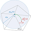 |
Figure 2. Illustration of the positioning noise as formulated in equation (7). For each node x of the mesh ∂Ωh, the initial noise-free boundary condition |


It should be noted that this approach only tackles the position inaccuracies of the robot, and not the orientation ones. In practice, the latter are expected to have a lower impact on the measurements, provided that the deployed microphone maintains the same properties at low incidence angles. In the experiments presented in Section 4, this is ensured by the fact that the used microphone (B&K 4190) is omnidirectionnal at all considered frequencies.
2.4.2 Impact on the error estimate
Considering our description of the positioning noise, the boundary conditions on ∂Ω are now given by
 (7)
(7)
where σ is a random vector containing three random variables, each following a Gaussian distribution of standard deviation σ P .
Substituting  for
for  in equation (6), the error estimate becomes
 (8)
(8)
It should be noted that the approximations of p appearing in equation (6),  , and equation (8),
  , are not derived from the same boundary density. Yet, the other terms involved in both estimates remain the same, as the perturbations are added to the measurements directly, and not to the boundary mesh.
Provided that the value of σ P is small in comparison to the mesh size h and to the wavelength λ, the L 2 norm involving the boundary conditions in equation (8) may be approximated by
 (9)
(9)
The error estimate of equation (8) then becomes
 (10)
(10)
with |σ| increasing linearly with σ P .
The last part of the right-hand term of equation (10) translates the two-fold impact of placement inaccuracies on the reconstruction error. First, the error now grows linearly with the value of σ P , and second, the previously expected 𝒪(h) convergence rate no longer holds, as the last term does not decrease with the mesh size h anymore.
3 Implementation and numerical simulations
As mentioned in the previous section, the versatility and convergence guarantees of BEM come at the cost of complex and resources consuming singular integral computations, and dense matrices factorization. However, benefiting from the rise of high performance parallel computing, FreeFEM [42] proposes a competitive implementation of BEM, relying on the hierarchical matrices’ computation tool HTool [43], and the parallel solvers proposed by PETSc [53]. Even though FreeFEM handles Lagrange element of order 0 to 2, it currently only supports linear surface elements, hence bounding the expected resolution performances. Despite the limitation identified in Section 2.3, the following results were obtained using P 1 Lagrange elements, as they offer a good trade-off between accuracy and computational cost, while allowing for a simplified mesh generation.
A numerical simulation of our BEM based SFE tool was thus implemented in order to assess our implementation agreement with the theoretically expected behaviors, as well as to infer good practices for our measurements setup. This simulation was also used as a mean to evaluate the actual impact of the robotic arm on the estimated acoustic pressure field. The measurements are simulated based on a regular acoustic dipole with a spacing of 0.45 m, whose analytical pressure field expression is sampled over a surrounding spherical mesh of diameter D = 0.5 m and varying size h. Each mesh is generated using a geodesic polyhedron primitive to ensure a uniform distribution of the vertices over the sphere.
The estimated sound field is then computed on a circular mesh of diameter 1 m, located in the z = 0 plane, and containing 100 nodes, for frequencies distributed between 100 Hz and 5000 Hz. The presented reconstruction errors are defined as the relative L 2 norm between the exact and estimated sound fields, computed over the whole circular mesh
 (11)
(11)
The procedure was repeated 20 times for various values of σ P ranging from 0.1 h to 2 h.
3.1 Agreement with theoretical error estimates
Given the choices of geometric and algebraic elements, the convergence rate of the computed solution towards the exact solution is theoretically expected to lay below 𝒪(h). This behavior was confirmed and even superseded by our numerical simulations, as a quadratic convergence rate was actually observed. The corresponding results are shown on Figure 3, where the reconstruction error is plotted against the product of the mesh size h and the wave number k.
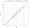 |
Figure 3. Reconstruction error obtained for measurements performed with increasing mesh sizes h. The dashedFrepeat line represents the actually observed 𝒪(h 2) convergence rate. |
As was nonetheless expected, the convergence tends to deteriorate when hk nears 10 [44], while the reconstruction error reaches 10% as hk increases towards 1. Enforcing a maximum estimation error of this magnitude, we indeed fall back on previously mentioned thumb rule of 6 measurements points per wavelength.
Despite the numerous advantages of a smaller mesh size, its practical value remains bounded by the minimal distance between two sensor positions, and is de facto constrained by the accuracy of the robot. A calibrated robot [26], with smaller positioning errors, will then allow for a finer mesh size, and a better reconstruction of the sound field, as was further discussed in Section 2.4.
3.2 Practical guidelines for the measurements setup
Whereas the agreement of our SFE tool with the expected error estimates provided an insight for the measurements density, their distance relative to the studied source remains to be discussed.
Provided that the mesh size satisfies k h ≤ 1, a larger mesh will provide a more spatially complete sampling of the sound field [34], and eventually reduce the estimation error. This hypothesis was confirmed by our simulations, as seen on Figure 4, with the reconstruction error decreasing with the diameter of the mesh D when the mesh size h remains constant and equal to 0.005 m.
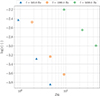 |
Figure 4. Reconstruction error obtained for measurements of an infinitesimal dipole performed on spheres of increasing diameters D. The measurements are assumed to be independent of the distance to the sound source. |
Remark that this numerical simulation does not take into account the physical aspects of real measurements, which heavily depend on the placement of microphones relative to the source. A microphone placed too far from the source will suffer from a high noise to signal ratio, and will be more likely to record reflected sound waves.
In practice, general guidelines [4] advise to place microphones on surfaces conformal to the studied object (i.e., at a similar distance to the studied object), at a distance (i) small in comparison to the studied object and (ii) small in comparison to the studied wavelength.
Finally, from a time-performance point of view, it should be recalled that both the dimensions and size of the measurements mesh directly impact the size of the linear system to solve, and thus the computational cost of the reconstruction algorithm. As shown in Table 1, the monitored computation time is found to increase quadratically with the ratio between the diameter of the mesh D and its size h, i.e., linearly with the number of measurements. For the lowest mesh size and highest mesh diameter, the reconstruction of the sought sound field may still take up to several minutes.
Monitored computation times for the reconstruction of the sound field generated by an infinitesimal dipole at 5 kHz, with increasing ratios between the mesh diameter and size  . Computations were run on the 4 cores of an Intel Core i5-4430 @ 3.00 GHz.
3.3 Impact of robotized measurements
In Section 2.4, two major effects of the robot positioning inaccuracies on the sound field estimation error were highlighted: a linear growth of the error with the value of σ P , and a decrease of the convergence rate with the mesh size h.
These two aspects were comforted by numerical simulations run on spherical meshes of diameter D = 0.5 m with varying mesh sizes h and positioning noise σ P . Both the highest and the average estimation errors obtained over the 20 draws are shown on Figure 5. As expected, these errors are found to broadly follow a linear trend, provided that the values of σP remains small in comparison to the mesh size h. The estimation errors obtained with σP = 0.0125 m, which is more than two times the mesh size h = 0.005 m, are indeed found to provide off trend results.
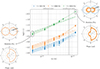 |
Figure 5. Reconstruction error obtained for measurements performed with a mesh size of 0.005 m and increasing values of positioning noise σ P . The dashed and dotted lines represents the expected 𝒪(σ P ) convergence rate for the highest and average reconstruction errors, respectively. The directivity patterns illustrate the results of the 20 draws at 5 kHz, for the smallest (left) and largest (right) values of σ P . |
For reasonable values of σP, but at higher frequencies, the reconstruction error seems to be more sensitive to the value of σP as well, with a more likely supra-linear trend. This observation highlights the increasing impact of positioning inaccuracies with the frequency, where a small misplacement of the microphone will lead to a large error in the sampling of the highly spatially varying sound field.
On the other hand, Figure 6 illustrates the degradation of the convergence rate, by reporting the average slope value of the reconstruction error curve with respect to the mesh size. As expected for both the average and highest estimation errors, the computed values are found to gradually decease from a quadratic trend to a sublinear one as the value of σP increases. Here too, the position noise sensitivity at higher frequencies is visible, as the decrease in the corresponding slopes values is seemingly steeper.
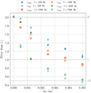 |
Figure 6. Evolution of the average slope value of the highest and average reconstruction error curves with respect to the mesh size, for measurements performed with increasing values of σ P . The dashed lines represent the corresponding quadratic, linear and sublinear trends. |
Studying the impact of the robot accuracy on the sound field estimation error is also an opportunity to highlight another benefit from a preliminary calibration of the robot. In the case of a Franka Robotics Panda robot, the calibration process allows to reduce the positioning error from 7.6 mm to 1.6 mm, which is a factor of 4.75 [26]. This reduction is expected to have a significant impact on the sound field estimation error, as shown in Figure 5. Assuming a linear decrease of the reconstruction error with the mesh size h, robot calibration has roughly the same impact as dividing the mesh size by 4.
4 Acoustic robotized measurements
Following the theoretical and numerical study of BEM as a mean to solve SFE problems, we may now proceed to the main experimental contribution of this paper: the introduction of a robotic arm to perform accurate tri-dimensional acoustic measurements in full autonomy. The details of the experimental setup, and the impact of the robot on the measurements are presented in this section.
4.1 Measurements setup
Drawing inspiration from previous works [22, 23], we designed a complete measurement setup (cf. Fig. 7) combining a Franka Robotics Panda serial robot, equipped with a 3D printed microphone prop, allowing the microphone to be held at a distance from the robot while performing the measurements. The 7 degrees of freedom of the serial robot allow for an increased maneuverability and a simplified collision avoidance, by offering multiple possible configurations for the same microphone position and orientation.
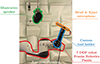 |
Figure 7. Robotized acoustic measurements setup. |
The handling of the robot kinematics and motion planning computation is overseen by the Moveit [54] library implemented in Robot Operating System (ROS) [55], released under open source licence. This library also offers off-the-shelf tools for self and external collision avoidance, and supports the addition of geometric constraints during inverse kinematics resolution. The latter asset was successfully exploited to free an additional degree of freedom associated to the rotation around the microphone axis, which does not impact the measurement. In this way, the robot may be controlled to autonomously and safely reach any user-defined position and orientation, with a continuous feedback on its current location.
On the microphone side, the support tool was designed to fit most Bruel & Kjaer and GRAS microphone pre-amplifiers. The acoustic measurements are handled by the measpy 2 Python library, which generically handles signals provided by classical sound cards, and National Instruments acquisition devices. In our current set up, a Bruel & Kjaer 4190 free-field microphone mounted on a GRAS 26AJ preamplifier were used, and recorded using a calibrated sound card.
All features were finally bundled up in a single ROS package robot_arm_acoustics 3, allowing to easily define the robotic cell collisions objects, and plan autonomous measurements routines along generic trajectories (circles, spheres, lines, etc.).
4.2 Robotized measurements validity hypothesis
The advantages in versatility and autonomy of the robotized measurements setup comes at the cost of a more complex measurement processing and inherently bulkier installation. To ensure the measurements quality, three hypotheses are derived, and assessed.
4.2.1 Hypothesis 1: Time-invariant sound source
In comparison to usual microphone-array-based measurements setups, where all acquisitions are performed simultaneously, robotized acoustic measurements are performed sequentially. As our work focuses on the study of electroacoustic measurements, where the response to an input signal is measured, this lack of synchronicity is not a problem as long as the transfer function between these correlated signals is computed.
In particular, our focus is set on the estimation of the sound field radiated by a JBL FLip 2, which was monaurally fed on its left channel with a white noise signal of 10 s, containing frequencies between f min = 10 Hz and f max = 20 kHz. The transfer functions between the recorded acoustic pressure (in Pa), and the signal generated by the sound card (in V) were then computed using Welch method [56], and smoothed over 1/12 octave bands.
Additionally, the behavior of the studied sound source must remain the same throughout the whole characterization process, by generating the same output signal for a given input signal. In other words, any measurement at a given location must generate the same results, regardless to the time at which it was performed. As this hypothesis heavily depends on the studied source, it was assessed experimentally by performing a series of three consecutive measurements with the robot fixed in the same configuration.
The obtained transfer functions and the corresponding modulus errors are displayed on Figure 8. The represented frequency range has been restricted between 50 Hz and 10 kHz, where the sound emitted by the loudspeaker is actually significant. The error between two complex transfer functions H1 and H2 is expressed as the logarithm of the modulus and phase of their ratio:
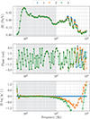 |
Figure 8. Time-invariability results obtained for the JBL FLip 2, with the robot set in the first control configuration of Figure A.1. The first two plots represent the computed transfer functions, and the last one the modulus error relative to the first (1) transfer function. The shaded zone highlights the frequency range where the absolute value of the error remains below 0.25 dB. |
where H 2 is the reference transfer function, and in our case, the first transfer function of the series.
The loudspeaker features a good time invariability, with an average error of 0.25 dB over the whole frequency range. Consequently, the hypothesis of a time-invariant sound source is considered verified for the studied loudspeaker.
4.2.2 Hypothesis 2: Low robot acoustic footprint
As the robot is not an acoustic transparent element, it will inherently impact the acoustic measurements. Although parasitic noise generated by the robot can be filtered during the transfer function computation, thanks to averaged measurements over a sufficiently long period of time [56], the robot acoustic footprint is more complex to handle, as it depends on the robot angular configuration.
As for the time invariability, our aim was to experimentally assess that the robot acoustic footprint is actually low enough to be neglected in the following. To achieve so, we performed two successive series of acoustic measurements, with the microphone rigidly held in the same position using pliers. For the first series, the robot is moved aside, so that its presence does not impact the acquisition. For the second one, it is placed as if it was holding the microphone in the very same position. As the microphone and its fixations are not shifted between the two series of measurements, their difference will only depend on the acoustic impact of the robot.
These two-fold series of measurements were performed at six so-called control configurations located around a JBL Flip 2 loudspeaker and displayed in appendix on Figure A.1. For each control configuration, the error between the transfer functions obtained with and without the robot is displayed on Figure 9.
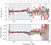 |
Figure 9. Robot acoustic footprint errors obtained for the six robot control configurations, relative to the robot-less transfer function. The shaded zone highlights the frequency range where the absolute value of the modulus error remains below 2.25 dB. |
Unlike the time-invariability results, the robot acoustic footprint has a non-negligible impact on the measurements, especially at higher frequencies. Yet, such behavior was expected: at lower frequencies, and larger wavelengths, the robot becomes small enough not to disturb the sound propagation. On the other hand, at higher frequencies and smaller wavelengths, the robot becomes a significant obstacle, and generates reflections of the incoming waves towards the microphone. As seen on Figure 9, this behavior becomes globally noticeable above f = 500 Hz, which corresponds to a wavelength of λ = 0.68 m, and is consistent with the robot dimensions. More specifically, Configurations (1) and (4) appear to be the most impactful, as the robot is the closest and most exposed to the sound source. Inversely, Configurations (2) and (6) have a lower impact on the measurements, as the robot is further away from the source, and exposes a smaller surface to the incoming waves.
Nevertheless, the deterioration caused by the robot induced reflections only seems to surge for frequencies above f = 1 kHz, and remains bounded at relatively acceptable levels below. Figure 9 indeed reports an amplitude error lower than 2.25 dB and a phase difference of 0.25 rad at its maximum below f = 1 kHz.
As the sounds generated by the loudspeaker become actually significant only above f = 50 Hz, the frequency range [50 Hz, 1 kHz] will be defined as the validity frequency range for our setup, within which measurements will be considered exploitable.
4.2.3 Hypothesis 3: Low robot positioning error
Although robotic arms are known for their high repeatability and maneuverability, their flawed accuracy for absolute positioning is often disregarded when used for metrology purposes. In this context however, an accurate sensor placement is of paramount importance [34], as it directly impacts the quality of the measurements: a misplaced microphone will fail to correctly capture the spatial variations of high frequency sound fields.
In order to guard us against this pitfall, an extended work has been carried out to ensure that the positioning accuracy of the Franka Robotics Panda used for our measurements remains lower than 2 mm [26].
If not completely removed, the actual impact of the remaining positioning errors on acoustic measurements cannot simply be assessed as for the previous hypothesis. Indeed, such a verification would require the ability to monitor the position and orientation of the microphone with a sub-millimetric accuracy, which would be difficult and impractical in our anechoic setup. Therefore, this hypothesis will be considered verified for the time being.
5 Experimental results
In order to assess the correct operation and performances of our robotized sound field estimation methodology, we applied the complete procedure to the acoustic characterization of an un-modeled JBL Flip 2 loudspeaker.
5.1 Experimental setup and Robotized measurements
Prior to the deployment of acoustic measurements, and to avoid any collisions between the robot and the loudspeaker, a 3D point cloud of the loudspeaker was recovered using an Intel RealSense D435 depth camera mounted on the robot flange. This point cloud allowed us to extract both a simple geometric description of the loudspeaker for collision avoidance, and its position and orientation relative to the robot base.
Based on the gathered geometric data, and in concordance with the guidelines described in Section 3.2, measurements were planned on a sphere of diameter 0.35 m, centered around the loudspeaker. At its closest point, the microphone will be located at a distance of roughly 0.05 m from the loudspeaker, which is small in comparison to the studied source dimensions, and to the minimal wavelength of the validity range identified in Section 4.2, λ min = 0.34 m. A mesh size of 0.025 m was chosen for the triangulation of the sphere, such that h k remains below 1 over the validity range.
The measurements were then autonomously performed according to the acquisition procedure of Section 4, by programming the robot to place the microphone successively at each vertex of the mesh, and align it with the local inward normal to the sphere.
Finally, the acquisition was concluded by 20 additional verification measurements, located on a circular mesh of diameter 0.5 m, lying in the horizontal z = 0 plane of the loudspeaker. The total duration as well as the number of measurements are reported in Table 2.
Detailed acquisition parameters for the JBL Flip 2 loudspeaker measurements.
It should be noted that the extended acquisition duration is mainly caused by the motion planning computations and executions, which both turned out to be slowed down because of the robot reduced speed, and complex collision avoidance trajectories.
The difference between the actual number of measurements, and the expected number of vertices is mostly caused by collision avoidance with the loudspeaker, or singular, unreachable robot poses. The missing measurements were recovered using an iterative hole-filling procedure, where each missing value is replaced by the averaged data of its direct neighbors. A statistical outliers’ removal step was also applied, assuming a normal distribution of the measured phase and amplitude over each vertex direct neighbors.
5.2 Sound field estimation results
Aiming to assess the conclusions of Section 3.1, two additional meshes were uniformly sub-sampled out of the initial measurements mesh. The detailed features of the three meshes are reported in Table 3, and an outlook of the corresponding measurements may be found in appendix on Figure B.1.
Details of the three meshes used for the sound field prediction.
The far-field acoustic pressure field was then estimated with the three measurements sets, using the BEM-based procedure presented in Section 2 and the circular verification mesh as the reconstruction domain. A sample of the detailed results obtained for the three meshes is shown on Figure 10.
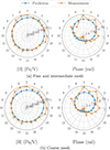 |
Figure 10. Predicted and measured acoustic pressure at f = 500 Hz, for the fine, intermediate and coarse meshes. At this frequency the results obtained for the fine and intermediate meshes are almost indistinguishable. |
At first sight, the reconstruction seems to correctly fit the measurements, with a faithful rendering of the left monaural directivity pattern of the loudspeaker. However, the SFE appears to have a smoothing effect on both the modulus and phase reconstructions, especially in comparison with the sharper verification measurements. Yet, this observation is not fully reliable, as the variations in measurements may also be caused by faulty acquisitions, or by the acoustic perturbations of the robot. Comparing the results obtained with the three meshes, it is actually not clear whether a finer resolution is beneficial, as the reconstructions slightly differ from one another, except for the coarse mesh phase prediction, which more clearly undervalued.
Taking a closer look at the evolution of the reconstruction errors with the frequency on Figure 11, the previous observation is confirmed: the three measurements sets provide very similar results, especially when comparing the intermediate and fine meshes, which are hardly distinguishable, even on the close-up view. The coarse mesh results appear slightly less accurate, whether within or outside the validity frequency range, but the difference still remains far from the predicted 4 times increase for a doubling of the mesh size (cf. Sect. 3.1).
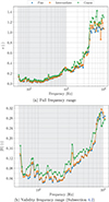 |
Figure 11. Reconstruction error, as defined in equation (11), for the fine, intermediate and coarse meshes. |
Considering the fine mesh, and as was expected with measurements performed at a fixed distance form one another, the reconstruction error globally increases with the frequency. In detail, the error remains below 15% for frequencies below 1 kHz but quickly rise to 30% around 1 kHz, and towards 100% when the validity frequency range is outreached, and the frequency reaches 5 kHz. Whereas the explosion of the estimation error at high frequencies, when h k exceeds 1, is in line with the expected behavior of the SFE tool, the sudden increase around 1 kHz is less so. It seems however to match the sharpening impact of the robot acoustic footprint at these frequencies (cf. Fig. 9), signaling a weakness in our second hypothesis.
By extension, the ill-compensated acoustic perturbations of the robot, combined with a still perfectible microphone placement could also explain the excessive similarity between the three measurements sets.
In the time being, and considering both the SFE results and the corresponding computation times reported in Table 4, the intermediate mesh seems to provide the best compromise between reconstruction accuracy and computational cost. Yet, the fine mesh is eventually expected to provide more accurate results, granted that the robot acoustic perturbations are properly accounted for.
Monitored computation times for the reconstruction of the sound field generated by the JBL Flip 2 at 5 kHz, for the coarse, intermediate and fine meshes. Computations were run on the 4 cores of an Intel Core i5-4430 @ 3.00 GHz.
6 Future work and conclusion
Throughout this paper, we tackled the problem of sound field estimation considering both the measurements and reconstruction aspects. The requirements for spatially dense and versatile acoustic measurements were met using a robotic arm, which also allows for a fully autonomous acquisition of the data. The impact of the robot on the measurements was assessed, and found to have non significant influence on the reconstruction provided that the studied source is sufficiently repeatable, the robot properly calibrated, and the studied frequencies remain below 1 kHz. This threshold is specific to the acoustically unshielded robotic arm used. For applications involving higher-frequency sources, such as industrial fans or small engines, the rest of the methodology remains numerically robust as long as the spatial sampling condition k h ≤ 1 is met. Future work, as discussed below, will aim to increase this frequency bound by minimizing the acoustic footprint of the robot.
The reconstruction was performed using a VBEM-based method, implemented using the BEM library provided by FreeFEM. This approach was found to be computationally efficient, and to provide accurate results, as the expected reconstruction error decreases quadratically with the mesh size, and linearly with the number of measurements. The estimation errors caused by the robot positioning inaccuracies were also studied. It was found to lower the expected convergence rate to the square root of the mesh size.
The overall procedure was finally tested on a commercial speaker, for which more than 2000 measurements were autonomously performed in less than 17 h. The agreement between estimated and measured acoustic pressure was assessed, showing a reconstruction error below 30% for frequencies below 1 kHz. However, the expected quadratic increase in the estimation error with the measurements spacing was not clearly observed, and erratic behaviors were noticed around 1 kHz, where the robot acoustic perturbations reach significant levels.
While BEM is computationally more demanding than expansion-based methods, the rise of parallel solvers ensures that computation times remain a small fraction of the total workflow. In our experiment, the overnight autonomous acquisition was followed by a reconstruction step taking less than 30 min on a standard workstation. The primary benefit is the reduction of human labor from several workdays to nearly zero, while maintaining the flexibility and lack of aliasing inherent to BEM.
The reconstruction error reaching 30% at the limit of the validity range must be interpreted in the context of a fully automated, unattended characterization of a complex and unknown source. Unlike laboratory setups with manual microphone placement, the error budget here includes robot-induced reflections and absolute positioning drift. This value is consistent with other experimental studies on complex radiators, where environmental noise and setup perturbations often lead to higher errors than those found in idealized simulations [2, 17, 57]. This deviation of experimental results from theoretical expectations highlights the necessity to improve the robot acoustic footprint. In this matter, both physical and numerical solutions can be considered.
On one hand, the application of foam on the robot surface could help dampen reflections at high frequencies, while increasing the distance between the robot body and the studied source during the acquisition could also reduce the amplitude of the reflected waves. Following the general guidelines provided by Wu [4] and Martinus [34], building a measurement mesh close and conformal to the studied object should also help to increase the signal to noise ratio. On the other hand, filtering techniques such as the wave separation method, or the time windowing technique [1], should be able to partially remove the robot perturbations, thanks to additional, but easily performed measurements. In particular, Gao et al. [58] and Langrenne et al. [59] investigated promising BEM based implementations of the wave separation method, using double layered measurements.
Concluding on the SFE part, the BEM implementation provided by FreeFEM would benefit from the use of higher-order surface elements, enabling the method to fully exploit higher-order Lagrange elements, as indicated in equation (6). Furthermore, deepening the possibilities offered by PETSc [53], the use of the minimization based solvers makes us confident in the possibility to tackle SFE dual NAH problem, whose inverse-problem nature might help to reduce SFE smoothing effect. In the sort-term, a more in-depth comparison with state-of-the-art SFE resolution methods such as HELS and ESM is also planned. On a more theoretical level, the quadratic convergence rates observed in our simulations call for a sharper reconstruction error estimate than equation (6), which could benefit from the finer geometric arguments of Nedelec [60].
Acknowledgments
Authors warmly thanks Thibault Toralba, Clément Yver and Clément Savaro for their help setting up the robotized measurements setup.
Funding
This work was partially supported by Carnot TSN, Carnot Mines, and Agence de l’Innovation de Défense – AID – via Centre Interdisciplinaire d’Études pour la Défense et la Sécurité – CIEDS – (project 2022 – Aéroacoustique des systémes multi-PROpulseurs pour les drones (APRO)).
Conflicts of interest
All authors declare that they have no conflicts of interest.
Data availability statement
Data are available on request from the authors.
References
- W. Klippel: Modeling and testing of loudspeakers used in sound-field control, in: Advances in Fundamental and Applied Research on Spatial Audio. IntechOpen, February 2022. [Google Scholar]
- F. Martinus, D.W. Herrin, J. Han: Identification of an aeroacoustic source using the inverse boundary element method. Noise Control Engineering Journal 58, 1 (2010) 83–92. [Google Scholar]
- H. Bi, F. Ma, T.D. Abhayapala, P.N. Samarasinghe: Spherical array based drone noise measurements and modelling for drone noise reduction via propeller phase control, in: 2021 IEEE Workshop on Applications of Signal Processing to Audio and Acoustics (WASPAA). New Paltz, NY, USA, October 2021, pp. 286–290. [Google Scholar]
- S.F. Wu: On reconstruction of acoustic pressure fields using the Helmholtz equation least squares method. The Journal of the Acoustical Society of America 107, 5 (2000) 2511–2522. [Google Scholar]
- D.W. Herrin, J. Liu, F. Martinus, D.J. Kato, S. Cheah: a. Noise Control Engineering Journal 58, 1 (2010) 74–82. [Google Scholar]
- M.B. Salin, D.A. Kosteev: Nearfield acoustic holography-based methods for far field prediction. Applied Acoustics 159 (2020) 107099. [Google Scholar]
- T. Shi, J. Stuart Bolton, W. Thor: Acoustic far-field prediction based on near-field measurements by using several different holography algorithms. The Journal of the Acoustical Society of America 151, 3 (2022) 2171–2180. [Google Scholar]
- C.-X. Bi, Y. Liu, Y.-B. Zhang, L. Xu: Sound field reconstruction using inverse boundary element method and sparse regularization. The Journal of the Acoustical Society of America 145, 5 (2019) 3154–3162. [Google Scholar]
- M. Hartenstein, F. Ollivier, M. Meinnel, H. Moingeon, C. Ollivon, A. Sokpoli, M. Pachebat, C. Pinhède, F. Silva, P. Luizard: Far-field directivity estimation with a cube-shaped array of 256 MEMS microphones, in: 53rd International Congress and Exposition on Noise Control Engineering (INTER-NOISE 2024), Nantes, France, August 2024. [Google Scholar]
- S.K. Chaitanya, K. Srinivasan: Equivalent source method based near field acoustic holography using multipath orthogonal matching pursuit. Applied Acoustics 187 (2022) 108501. [Google Scholar]
- C. Sugiyama, K. Itoyama, K. Nishida, K. Nakadai: Assessment of simultaneous calibration for positions, orientations, and time offsets in multiple microphone arrays systems, in: 2023 IEEE/SICE International Symposium on System Integration (SII). Atlanta, GA, USA, January 2023, pp. 1–6. [Google Scholar]
- Z. Havranek, P. Benes, S. Klusacek: Application of mems microphone array for acoustic holography, in: Proceedings of the 10th European Conference on Noise Control, Euronoise 2015. Maastricht, Netherlands, May 2015, pp. 919–924. [Google Scholar]
- I. Lopez Arteaga, R. Scholte, H. Nijmeijer: Improved source reconstruction in Fourier-based Near-field Acoustic Holography applied to small apertures. Mechanical Systems and Signal Processing 32 (2012) 359–373. [Google Scholar]
- M. Aucejo, N. Totaro, J.-L. Guyader: Identification of source velocities on 3D structures in non-anechoic environments: theoretical background and experimental validation of the inverse patch transfer functions method. Journal of Sound and Vibration 329, 18 (2010) 3691–3708. [CrossRef] [Google Scholar]
- M. Szczodrak, A. Kurowski, J. Kotus, A. Czyżewski, B. Kostek: A system for acoustic field measurement employing cartesian robot. Metrology and Measurement Systems 23, 3 (2016) 333–343. [Google Scholar]
- S. Forget, N. Totaro, J.L. Guyader, M. Schaeffer: Source fields reconstruction with 3D mapping by means of the virtual acoustic volume concept. Journal of Sound and Vibration 381 (2016) 48–64. [CrossRef] [Google Scholar]
- H. Vold, P. Shah, J. Davis, P. Bremner, D. McLaughlin, P. Morris, J. Veltin, R. McKinley: High resolution continuous scan acoustical holography applied to high-speed jet noise, in: 16th AIAA/CEAS Aeroacoustics Conference, Stockholm, Sweden, June 2010. [Google Scholar]
- Z.-W. Luo, D. Fernandez Comesana, C.-J. Zheng, C.-X. Bi: A free field recovery technique based on the boundary element method and three-dimensional scanning measurements. The Journal of the Acoustical Society of America 150, 5 (2021) 3929–3948. [Google Scholar]
- M. Legg, S. Bradley: A combined microphone and camera calibration technique with application to acoustic imaging. IEEE Transactions on Image Processing 22, 10 (2013) 4028–4039. [Google Scholar]
- D. Li, H. Wu, Y. Zha, W. Jiang: A sound source reconstruction approach based on the machine vision and inverse patch transfer functions method. Applied Acoustics 181 (2021) 108180. [Google Scholar]
- Y. Bernhardt, D. Solodov, D. Müller, M. Kreutzbruck: Listening for airborne sound of damage: a new mode of diagnostic imaging. Frontiers in Built Environment 6 (2020) 66. [Google Scholar]
- J. Walker, I.W. Foged: Robotic methods in acoustics: Analysis and fabrication processes of sound scattering acoustic panels, in: 36th eCAADe Conference. Vol. 1. Lodz, Poland, 2018, pp. 835–840. [Google Scholar]
- M. Nolan, S.A. Verburg, J. Brunskog, E. Fernandez-Grande: Experimental characterization of the sound field in a reverberation room. The Journal of the Acoustical Society of America 145, 4 (2019) 2237–2246. [Google Scholar]
- M. Kefer, Q. Lu: Acoustic holography – a robot application, in: 2016 IEEE International Conference on Real-time Computing and Robotics (RCAR). Angkor Wat, Cambodia, June 2016, pp. 312–316. [Google Scholar]
- N. Totaro, M. Robin, J. Rassez, M.-A. Malinge: Robotic arm, 3D vision and geometric matching for an efficient implementation of inverse Patch Transfer Function method, in: 53rd International Congress and Exposition on Noise Control Engineering (INTER-NOISE 2024), Nantes, France, August 2024. [Google Scholar]
- C. Pascal, A. Chapoutot, O. Doaré: A ros-based kinematic calibration tool for serial robots, in: 2023 IEEE/RSJ International Conference on Intelligent Robots and Systems (IROS), Detroit, MI, USA, October 2023. [Google Scholar]
- J.D. Maynard, E.G. Williams, Y. Lee: Nearfield acoustic holography: I. Theory of generalized holography and the development of NAH. The Journal of the Acoustical Society of America 78, 4 (1985) 1395–1413. [Google Scholar]
- J. Hald: Basic theory and properties of statistically optimized near-field acoustical holography. The Journal of the Acoustical Society of America 125, 4 (2009) 2105–2120. [Google Scholar]
- N.P. Valdivia: Advanced equivalent source methodologies for near-field acoustic holography. Journal of Sound and Vibration 438 (2019) 66–82. [Google Scholar]
- T. Semenova, S.F. Wu: On the choice of expansion functions in the Helmholtz equation least-squares method. The Journal of the Acoustical Society of America 117, 2 (2005) 701–710. [Google Scholar]
- A. Canclini, M. Varini, F. Antonacci, A. Sarti: Dictionary-based equivalent source method for near-field acoustic holography, in: 2017 IEEE International Conference on Acoustics, Speech and Signal Processing (ICASSP). New Orleans, LA, USA, March 2017, pp. 166–170. [Google Scholar]
- J. Antoni: A Bayesian approach to sound source reconstruction: optimal basis, regularization, and focusing. The Journal of the Acoustical Society of America 131, 4 (2012) 2873–2890. [Google Scholar]
- E.G. Williams: Regularization methods for near-field acoustical holography. The Journal of the Acoustical Society of America 110, 4 (2001) 1976–1988. [Google Scholar]
- F. Martinus, D.W. Herrin, A.F. Seybert: Selecting measurement locations to minimize reconstruction error using the inverse boundary element method. Journal of Computational Acoustics 15, 4 (2007) 531–555. [Google Scholar]
- J. Hald: Fast wideband acoustical holography. The Journal of the Acoustical Society of America 139, 4 (2016) 1508–1517. [Google Scholar]
- G. Chardon, L. Daudet, A. Peillot, F. Ollivier, N. Bertin, R. Gribonval: Near-field acoustic holography using sparse regularization and compressive sampling principles. The Journal of the Acoustical Society of America 132, 3 (2012) 1521–1534. [CrossRef] [PubMed] [Google Scholar]
- L.L. Thompson: A review of finite-element methods for time-harmonic acoustics. The Journal of the Acoustical Society of America 119, 3 (2006) 1315–1330. [Google Scholar]
- M.R. Bai: Application of BEM (boundary element method)-based acoustic holography to radiation analysis of sound sources with arbitrarily shaped geometries. The Journal of the Acoustical Society of America 92, 1 (1992) 533–549. [Google Scholar]
- A. Alguacil, M. Bauerheim, M.C. Jacob, S. Moreau: Predicting the propagation of acoustic waves using deep convolutional neural networks. Journal of Sound and Vibration 512 (2021) 116285. [Google Scholar]
- M. Olivieri, M. Pezzoli, F. Antonacci, A. Sarti: A physics-informed neural network approach for nearfield acoustic holography. Sensors 21, 23 (2021) 7834. [Google Scholar]
- K. Shigemi, S. Koyama, T. Nakamura, H. Saruwatari: Physics-informed convolutional neural network with bicubic spline interpolation for sound field estimation, in: 2022 International Workshop on Acoustic Signal Enhancement (IWAENC). Bamberg, Germany, September 2022, 1–5. [Google Scholar]
- F. Hecht: New development in FreeFem++. Journal of Numerical Mathematics 20, 3, 4 (2012) 251–265. [Google Scholar]
- P. Marchand: Schwarz Methods and Boundary Integral Equations. Theses, Sorbonne Université, January 2020. [Google Scholar]
- S.A. Sauter, C. Schwab: Boundary Element Methods. Vol. 39 of Springer Series in Computational Mathematics. Springer, Berlin, Heidelberg, 2011. [Google Scholar]
- S. Kirkup: The boundary element method in acoustics: a survey. Applied Sciences 9, 8 (2019) 1642. [CrossRef] [Google Scholar]
- N. Valdivia, E. Williams: Implicit methods of solution to integral formulations in boundary element method based nearfield acoustic holography. Acoustical Society of America Journal 116 (2004) 1559–1572. [Google Scholar]
- A. Schuhmacher, J. Hald, K.B. Rasmussen, P.C. Hansen: Sound source reconstruction using inverse boundary element calculations. The Journal of the Acoustical Society of America 113, 1 (2003) 114–127. [CrossRef] [PubMed] [Google Scholar]
- S.T. Raveendra, N. Vlahopoulos, A. Glaves: An indirect boundary element formulation for multi-valued impedance simulation in structural acoustics. Applied Mathematical Modelling 22, 6 (1998) 379–393. [Google Scholar]
- H. Brakhage, P. Werner: Über das dirichletsche außenraumproblem für die helmholtzsche schwingungsgleichung. Archiv der Mathematik 16, 1 (1965) 325–329. [Google Scholar]
- P.G. Ciarlet, P.A. Raviart: Interpolation theory over curved elements, with applications to finite element methods. Computer Methods in Applied Mechanics and Engineering 1, 2 (1972) 217–249. [Google Scholar]
- S. Marburg: Six boundary elements per wavelength: Is that enough? Journal of Computational Acoustics 10 (2002) 25–51. [Google Scholar]
- B.K. Gardner, R.J. Bernhard: A noise source identification technique using an inverse Helmholtz integral equation method. Journal of Vibration, Acoustics, Stress, and Reliability in Design 110, 1 (1988) 84–90. [Google Scholar]
- S. Balay, W. Gropp, L.C. McInnes, B.F. Smith: PETSC, the portable, extensible toolkit for scientific computation. Argonne National Laboratory 2, 17 (1998). [Google Scholar]
- D. Coleman, I.A. Sucan, S. Chitta, N. Correll: Reducing the barrier to entry of complex robotic software: a moveit! case study. Journal on Software Engineering for Robotics 5, 1 (2014) 3–16. [Google Scholar]
- M. Quigley, K. Conley, B. Gerkey, J. Faust, T. Foote, J. Leibs, R. Wheeler, A.Y. Ng: ROS: an open-source robot operating system, in: ICRA Workshop on Open Source Software. Vol. 3. Kobe, Japan, May 2009, p. 5. [Google Scholar]
- P.D. Welch: The use of fast Fourier transform for the estimation of power spectra: a method based on time averaging over short, modified periodograms. IEEE Transactions on Audio and Electroacoustics 15, 2 (1967) 70–73. [CrossRef] [Google Scholar]
- Z.-W. Luo, D. Fernandez Comesana, C.-J. Zheng, C.-X. Bi: Near-field acoustic holography with three-dimensional scanning measurements. Journal of Sound and Vibration 439 (2019) 43–55. [Google Scholar]
- H. Gao, Q. Zhu, S. Liu, P. Xing, G. Li: The formulations based on the indirect boundary element method for the acoustic characterization of an arbitrarily shaped source in a bounded noisy environment. Engineering Analysis with Boundary Elements 138 (2022) 65–82. [Google Scholar]
- C. Langrenne, M. Melon, A. Garcia: A boundary element method for near-field acoustical holography in bounded noisy environment. The Journal of the Acoustical Society of America 123, 5_Supplement (2008) 3309. [Google Scholar]
- J.C. Nedelec: Curved finite element methods for the solution of singular integral equations on surfaces in R3. Computer Methods in Applied Mechanics and Engineering 8, 1 (1976) 61–80. [Google Scholar]
Appendix A
Robot configurations
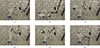 |
Figure A.1. Robot control configurations for sound source time invariance and robot acoustic footprint assessment. |
Appendix B
Post-processed measurements
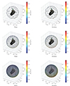 |
Figure B.1. Example of post-processed measurements at f = 500 Hz, for the coarse, intermediate and fine meshes. |
Cite this article as: Pascal C. Marchand P. Chapoutot A. & Doaré O. 2026. Automated Sound Field Estimation combining robotized acoustic measurements and the boundary elements method. Acta Acustica, 10, 25. https://doi.org/10.1051/aacus/2026017.
All Tables
Monitored computation times for the reconstruction of the sound field generated by an infinitesimal dipole at 5 kHz, with increasing ratios between the mesh diameter and size . Computations were run on the 4 cores of an Intel Core i5-4430 @ 3.00 GHz.
Monitored computation times for the reconstruction of the sound field generated by the JBL Flip 2 at 5 kHz, for the coarse, intermediate and fine meshes. Computations were run on the 4 cores of an Intel Core i5-4430 @ 3.00 GHz.
All Figures
|
Figure 1. Dirichlet exterior problem for the Helmholtz equation. |
| In the text | |
|
Figure 2. Illustration of the positioning noise as formulated in equation (7). For each node x of the mesh ∂Ωh, the initial noise-free boundary condition |
| In the text | |
|
Figure 3. Reconstruction error obtained for measurements performed with increasing mesh sizes h. The dashedFrepeat line represents the actually observed 𝒪(h 2) convergence rate. |
| In the text | |
|
Figure 4. Reconstruction error obtained for measurements of an infinitesimal dipole performed on spheres of increasing diameters D. The measurements are assumed to be independent of the distance to the sound source. |
| In the text | |
|
Figure 5. Reconstruction error obtained for measurements performed with a mesh size of 0.005 m and increasing values of positioning noise σ P . The dashed and dotted lines represents the expected 𝒪(σ P ) convergence rate for the highest and average reconstruction errors, respectively. The directivity patterns illustrate the results of the 20 draws at 5 kHz, for the smallest (left) and largest (right) values of σ P . |
| In the text | |
|
Figure 6. Evolution of the average slope value of the highest and average reconstruction error curves with respect to the mesh size, for measurements performed with increasing values of σ P . The dashed lines represent the corresponding quadratic, linear and sublinear trends. |
| In the text | |
|
Figure 7. Robotized acoustic measurements setup. |
| In the text | |
|
Figure 8. Time-invariability results obtained for the JBL FLip 2, with the robot set in the first control configuration of Figure A.1. The first two plots represent the computed transfer functions, and the last one the modulus error relative to the first (1) transfer function. The shaded zone highlights the frequency range where the absolute value of the error remains below 0.25 dB. |
| In the text | |
|
Figure 9. Robot acoustic footprint errors obtained for the six robot control configurations, relative to the robot-less transfer function. The shaded zone highlights the frequency range where the absolute value of the modulus error remains below 2.25 dB. |
| In the text | |
|
Figure 10. Predicted and measured acoustic pressure at f = 500 Hz, for the fine, intermediate and coarse meshes. At this frequency the results obtained for the fine and intermediate meshes are almost indistinguishable. |
| In the text | |
|
Figure 11. Reconstruction error, as defined in equation (11), for the fine, intermediate and coarse meshes. |
| In the text | |
|
Figure A.1. Robot control configurations for sound source time invariance and robot acoustic footprint assessment. |
| In the text | |
|
Figure B.1. Example of post-processed measurements at f = 500 Hz, for the coarse, intermediate and fine meshes. |
| In the text | |
Current usage metrics show cumulative count of Article Views (full-text article views including HTML views, PDF and ePub downloads, according to the available data) and Abstracts Views on Vision4Press platform.
Data correspond to usage on the plateform after 2015. The current usage metrics is available 48-96 hours after online publication and is updated daily on week days.
Initial download of the metrics may take a while.