| Issue |
Acta Acust.
Volume 10, 2026
Topical Issue - Modern approaches to Active Control of Sound and Vibration
|
|
|---|---|---|
| Article Number | 22 | |
| Number of page(s) | 14 | |
| DOI | https://doi.org/10.1051/aacus/2026018 | |
| Published online | 03 April 2026 | |
Scientific Article
Optimisation of the spatial configuration of microphones for robust virtual sensing in a diffuse sound field
Institute of Sound and Vibration Research, University of Southampton, University Rd., Southampton, SO17 1BJ UK
* Corresponding author: This email address is being protected from spambots. You need JavaScript enabled to view it.
Received:
30
December
2025
Accepted:
18
February
2026
Abstract
Virtual sensing methods are utilised in active noise control systems where the error sensors cannot be placed at the locations where control is physically required. Their performance critically depends on the spatial configuration of the physical monitoring microphones used to estimate the pressures at the virtual error sensor locations. This paper investigates the use of a genetic algorithm to calculate optimal microphone placements for estimation within a stationary diffuse sound field. A multi-objective optimisation framework is formulated, simultaneously minimising the estimation error and the condition number of the monitoring microphone power spectral density matrix, thereby addressing both estimation accuracy and robustness to uncertainties. Optimisations are carried out for a single frequency and for three representative frequencies spanning three octaves. The resulting Pareto fronts reveal the inherent trade-off between performance and numerical stability. The Technique for Order of Preference by Similarity to Ideal Solution is applied to select a single optimal solution from each Pareto set. These solutions achieve a balanced compromise, offering a small reduction in estimation performance while reducing the condition number by up to an order of magnitude compared with configurations that solely minimise the error. The minimum error and optimal solutions are evaluated over a broad frequency range, where the optimal designs are shown to significantly reduce the conditioning for a modest increase in estimation errors. The study highlights characteristic spatial patterns that promote optimal performance, and demonstrates the effectiveness of a genetic algorithm-based multi-objective optimisation for designing robust microphone configurations for virtual sensing applications.
Key words: Virtual sensing / Remote microphone technique / Microphone arrays / Genetic algorithm / Optimisation
© The Author(s), Published by EDP Sciences, 2026
 This is an Open Access article distributed under the terms of the Creative Commons Attribution License (https://creativecommons.org/licenses/by/4.0), which permits unrestricted use, distribution, and reproduction in any medium, provided the original work is properly cited.
1 Introduction
In the context of Active Noise Control (ANC), Virtual Sensing (VS) enables control to be achieved at positions that are remote from physical sensors [1] and has been found to increase control performance in such situations [2, 3]. However, it has been demonstrated that the utilised physical microphone configuration significantly affects the estimation performance of the VS system [3, 4], and this constitutes one of the limiting factors for the overall control performance [5].
The estimation accuracy provided by a VS system is governed by the coherence between the sound field at the physical monitoring microphones and the remote locations [6]. Augmenting the measurements with pressure gradient information can increase the coherence between distant positions and has been shown to improve estimation accuracy in both diffuse [4, 7, 8] and directional [3, 9] sound fields. It has been demonstrated that the estimation performance increases along the axis of the pressure gradient [4], and the use of microphone configurations that estimate pressure gradient along three axes [10] can provide estimation performance gains in all three dimensions. Although this approach can work as a guideline to design VS systems with increased estimation performance compared to conventional arrays, configurations of closely spaced microphones can significantly increase the sensitivity to practical perturbations [3, 4], dictating the need for dedicated pressure gradient sensors [7, 8].
In many practical applications, the monitoring microphone positions are largely dictated by the spatial constraints of the system and configurations such as those described in the previous paragraph may not even be realisable. Due to such practical limitations, many studies have focused on the investigation of rather simple and straightforward configurations, such as linear, circular or spherical arrays [3, 4, 6, 9], or arbitrary arrays with microphones positioned based on the physical constraints [11].
In search for optimal microphone positions, various optimisation methods have been proposed in the literature. Krauss et al. [12] proposed a sensor placement method where the sensors were placed at positions that maximise the mutual information between the selected positions and the rest of the positions in the domain of interest. In the original formulation, the spatial distribution of the phenomena was assumed to be Gaussian, in an extension of the method introduced by Kentaro et al. [13], the sound-field kernel [14] was used to formulate the covariance matrix between the measured responses and, assuming statistical independence between frequencies, broadband disturbances were treated by summing the contributions across frequency. The method was shown to outperform the original in simulations of plane waves. Chardon et al. [15] proposed the definition of microphone geometries on the boundary of the domain of interest with the addition of sensors inside the domain to stabilise the interpolation of the sound field. They used the empirical interpolation method [16], a general interpolation method introduced in the context of partial differential equations, to calculate points for arbitrarily shaped domains. Koyama et al. [17] extended the method to jointly calculate the sensor and source positions for sound field control. In a different study [18], the same authors evaluated the performance of four microphone placement methods, including some of those mentioned above, in the context of sound field control, via simulations for both tonal and broadband excitations. Overall, optimal placement methods provided better control performance compared to conventional, uniformly spaced sensor configurations. Verburg et al. [19] defined the problem of picking optimal microphone positions in a Bayesian probabilistic estimation framework, where they investigated the estimation performance of microphone configurations optimally derived for pressure reconstruction, or sound field parameter estimation. The methods were evaluated in simulations, and it was found that configurations derived for pressure reconstruction positioned multiple sensors close to the estimation area and were found to provide superior estimation accuracy.
In a different approach to the calculation of optimal sensor positions evolutionary algorithms such as the Genetic Algorithm (GA) [20] or the Memetic Algorithm (MA) [20, 21] have found use mainly for the investigation of the optimal placement of sensors, actuators and masses on structures for Active Structural Acoustic Control (ASAC) [22–25]. Wrona et al. [26] utilised an MA to calculate optimal sensor and control source positions to minimise the average spatial distribution of noise in a specified area, shaping Zones-of-Quiet (ZoQ) in an enclosure. In a different study, Zhang et al. [27] used a GA to calculate the monitoring configuration with the smallest possible number of microphones that results in wideband estimation accuracy.
In a large number of studies found in the literature, including those discussed in the preceding paragraphs, optimal configurations are calculated based on a predefined set of positions, with the algorithm searching through the possible combinations and selecting the best based on a defined optimality criterion. The current work investigates the use of the GA in calculating optimal VS microphone configurations for the estimation of the pressures in a diffuse field, using the Remote Microphone Technique (RMT) [1]. Formulating the problem of calculating microphone configurations for sound field estimation as a Multi-Objective Optimisation (MOO) problem enables the calculation of configurations that optimally compromise between multiple objectives [28]. For example, contrary to most studies discussed earlier, which collapse multi-frequency performance into a single scalar metric, the approach used in this work calculates a series of solutions with varying degrees of performance at each frequency. A single optimal configuration can then be selected that satisfies the required trade-offs of a practical system. The work expands on a preliminary study carried out by the authors [29] by defining a MOO problem over an ensemble of frequencies. MOO constitutes a valid approach when the metrics characterising the performance of a system cannot be completely ordered, and thus no single value can quantify the global optimal solution [30]. In the current work, MOO is used to calculate solutions that excel at potentially conflicting metrics, namely the estimation performance and the robustness to uncertainties. The aim is to calculate optimal monitoring microphone configurations and identify spatial patterns that optimise the system characteristics.
The article is structured as follows: Section 2 presents the formulation of the estimation problem and Section 3 the structure of the GA. Section 4 describes how a single optimal solution is selected from a set of solutions that optimise the combination of the minimisation parameters, and Section 5 describes the optimisation simulations and their results. The most important findings are discussed, and the article concludes with a summary in Section 6.
2 Remote microphone virtual sensing
In the RMT, measurements of the sound field at physical monitoring microphones are filtered by an observation filter to produce an estimate of the sound field at some remote locations, defined by virtual microphones [1]. The block diagram of the VS system used in the current work is depicted in Figure 1. The disturbance fields  , at Nm monitoring microphones, and
  at Ne virtual microphones, are generated by Nv sources with complex strengths
  through the transfer functions
  and
and  . The notation [ ⋅ ]T denotes transposition, and the frequency dependence of the disturbance field has been omitted for brevity. All signals are assumed to be realisations of wide-sense stationary processes and are completely characterised by their power and cross-spectral densities.
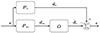 |
Figure 1. Block diagram of a remote microphone virtual sensing system. An observation filter, |


The estimate of the disturbance field at the virtual microphone locations,  , is acquired by filtering the monitoring microphone responses, dm, with the observation filter
  , which gives
 (1)
(1)
where ![Mathematical equation: $ \left[ \, \hat{\cdot} \, \right] $](/articles/aacus/full_html/2026/01/aacus250219/aacus250219-eq14.gif) denotes an estimated quantity. The estimation error is defined as the difference between the true and estimated responses at the virtual microphone locations and is given by
denotes an estimated quantity. The estimation error is defined as the difference between the true and estimated responses at the virtual microphone locations and is given by
 (2)
(2)
The optimal linear observation filter minimises the mean squared error, E[ ϵ H ϵ ], where E[ ⋅ ] denotes the expectation operator, and [ ⋅ ]H denotes Hermitian transposition, and is given by Elliott et al. [31]
 (3)
(3)
where matrix inversion is denoted by [ ⋅ ]−1, I is an Nm × Nm identity matrix and β is a regularisation parameter that constrains the maximum values of the filter decreasing its sensitivity to noise or uncertainty [3, 32] and can be frequency dependent; Sme is the Cross-Spectral Density (CSD) matrix between the monitoring and virtual microphone responses, and S mm is the Power Spectral Density (PSD) matrix of the monitoring microphone responses, both given as
![Mathematical equation: $$ \begin{aligned} {\boldsymbol{S}}_{\mathrm{me} }&= \mathrm{E} \!\left[ {\boldsymbol{d}}_{\mathrm{e} } {\boldsymbol{d}}_{\mathrm{m} }^{\mathrm{H} } \right] = {\boldsymbol{P}}_{\mathrm{e} } {\boldsymbol{S}}_{\mathrm{vv} } {\boldsymbol{P}}_{\mathrm{m} }^{\mathrm{H} } \end{aligned} $$](/articles/aacus/full_html/2026/01/aacus250219/aacus250219-eq20.gif) (4)
(4)
![Mathematical equation: $$ \begin{aligned} {\boldsymbol{S}}_{\mathrm{mm} }&= \mathrm{E} \!\left[ {\boldsymbol{d}}_{\mathrm{m} } {\boldsymbol{d}}_{\mathrm{m} }^{\mathrm{H} } \right] = {\boldsymbol{P}}_{\mathrm{m} } {\boldsymbol{S}}_{\mathrm{vv} } {\boldsymbol{P}}_{\mathrm{m} }^{\mathrm{H} } , \end{aligned} $$](/articles/aacus/full_html/2026/01/aacus250219/aacus250219-eq21.gif) (5)
(5)
where Svv is the PSD matrix of the source strengths given by
![Mathematical equation: $$ \begin{aligned} {\boldsymbol{S}}_{\mathrm{vv} } = \mathrm{E} \!\left[ {\boldsymbol{v}} {\boldsymbol{v}}^{\mathrm{H} } \right]. \end{aligned} $$](/articles/aacus/full_html/2026/01/aacus250219/aacus250219-eq23.gif) (6)
(6)
With the CSD and PSD matrices being distinct for each frequency, the observation filter given by equation (3) must be calculated for each frequency of interest.
Calculation of the optimal observation filter requires the inversion of the monitoring microphone PSD matrix, Smm, which can be ill-conditioned, rendering the system sensitive to uncertainties [3, 5, 11]. The condition number of the matrix is used to quantify the sensitivity of the system to perturbations and is calculated as
 (7)
(7)
where ∥ ⋅ ∥ 2 denotes the 2-norm, and σmax and σmin the largest and smallest singular values of Smm, respectively. In this study, the observation filter and estimation error were calculated under ideal, noise-free conditions. Consequently, large condition numbers indicate a highly sensitive filter and suggest that the resulting estimation errors are unlikely to be attainable in practical implementations.
The condition number can be variously affected by regularisation, as in equation (3), or by the geometry of the monitoring microphone configuration [4]. In particular, careful placement of the monitoring microphones can reduce the correlation between their responses and lower the condition number of the PSD matrix. The focus of the current study is to investigate the feasibility of deploying robust monitoring microphone configurations while preserving high estimation accuracy, without the use of significant numerical regularisation.
To minimise numerical errors, in the current work, a frequency-dependent regularisation factor is introduced, based on the signal-dependent approach utilised in [32, 33], which is given by
 (8)
(8)
where ∥ ⋅ ∥F denotes the Frobenius norm and n is the normalised root mean square “noise” term. The regularisation factor, calculated as in equation (7) with a constant, frequency-independent n value, guarantees a uniform signal-to-noise ratio across frequencies. This facilitates evaluation of the effect of the array geometry on the estimation performance, while mitigating extreme numerical instabilities in the inversion of the PSD matrix in equation (3) at frequencies where it becomes ill-conditioned.
3 The genetic algorithm
The GA is one of many heuristic algorithms proposed in the literature to solve global optimisation problems [20]. A population of solutions evolves over generations, approaching the optimal solution. The performance of each solution, termed fitness, is determined by a user-defined fitness function that the GA tries to minimise, or maximise. In the case of MOO problems, a vector-valued fitness function is introduced, and instead of a single solution, an ensemble of optimal solutions, termed the Pareto set, is calculated. Each solution in the Pareto set is optimal in the sense that no other calculated solution achieves a better score for at least one of the objectives without sacrificing performance on another [34]. When the Pareto set is acquired, a different optimality criterion can be used to select a single solution providing an acceptable trade-off between the performance metrics. The built-in MATLAB™ GA [35] is used in this work, with Figure 2 showing the logic diagram – each step is described in the following sections. The parameter values used to implement the GA, such as the population size and encoding, selection, mutation and crossover operators, and the number of solutions created through crossover and mutation, were selected based on results from the preliminary study [29] and initial trials performed with the GA described here.
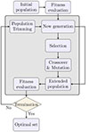 |
Figure 2. The logic diagram of a genetic algorithm. A random initial population is generated and its individuals are crossed over and mutated to create a new generation. When a stop criterion is met, the optimisation is terminated. |
3.1 Initial population and coding scheme
In order to implement the optimisation process, it is first necessary to encode the optimisation parameters, or genes, which constitute the genome of each solution. In this work, the genes represent two-dimensional microphone coordinates, interleaved in vector form with each genome being represented as  , with xi and yi the coordinates of the ith microphone. It is worth noting that, contrary to prior studies [18, 19, 22–27], the parameter space here is continuous.
To facilitate the search of as large a part of the parameter space as possible, which was shown to exhibit a large number of extrema [29], a large population comprising 500 individuals was used. To enable comparison with the preliminary research reported in Kappis and Cheer [29] and provide “guidance” to the algorithm, the two solutions that provided the best estimation performance in these initial simulations were included in the initial population. The rest of the individuals forming the initial population are drawn from a multivariate scaled and shifted uniform random distribution to satisfy any constraints. Individuals that do not satisfy non-linear constraints are discarded, and a minimum infeasibility problem is solved to generate feasible solutions. The constraints are problem-specific and are described in Section 5.1.
3.2 Fitness function
The fitness functions used here reflect the two characteristics of the VS system that should be minimised: the estimation error and the sensitivity to uncertainties. The estimation performance is calculated as the sum of the Normalised Mean Squared Errors (NMSE) at the virtual microphone positions, given by
 (9)
(9)
with tr{ ⋅ } denoting the matrix trace operator, and ![Mathematical equation: $ {\boldsymbol S}_{\epsilon \epsilon} \!\left( f \right) = \mathrm{E} \!\left[ {\boldsymbol{\epsilon}} \!\left( f \right) {\boldsymbol{\epsilon}}^{\mathrm{H}} \!\left( f \right) \right] $](/articles/aacus/full_html/2026/01/aacus250219/aacus250219-eq30.gif) and
and ![Mathematical equation: $ {\boldsymbol S}_{\mathrm{ee}} \!\left( f \right) = \mathrm{E} \!\left[ {\boldsymbol d}_{\mathrm{e}} \!\left( f \right) {\boldsymbol d}_{\mathrm{e}}^{\mathrm{H}} \!\left( f \right) \right] $](/articles/aacus/full_html/2026/01/aacus250219/aacus250219-eq31.gif) the PSD matrices of the errors and virtual microphone responses, respectively. The metric assigns large negative values for good estimation, with −∞ denoting perfect estimation.
the PSD matrices of the errors and virtual microphone responses, respectively. The metric assigns large negative values for good estimation, with −∞ denoting perfect estimation.
The NMSE in equation (8) is calculated for each frequency of interest. A different metric, encountered in multiple methods proposed in the literature [18, 19], results from the sum of the NMSEs across frequency as
 (10)
(10)
where Nf denotes the number of frequencies. Although equation (9) does not directly represent the broadband performance of the VS system, it is used here to compare the solutions provided by optimisation at distinct frequencies compared to their sum.
The sensitivity of the system to uncertainties is quantified by the condition number defined in equation (6), evaluated at each frequency like
 (11)
(11)
Similar to the NMSE above, the sum of the condition numbers over frequency can also be used, which is given by
 (12)
(12)
The metrics defined by equations (8)–(11) are combined to define the vector-valued fitness functions used in this work, described in the respective sections in Section 5. All metrics are defined so that lower values indicate better performance; therefore, the optimisation task is to find the arguments that minimise the fitness function.
If an individual violates any constraints, its fitness value is penalised. It is assigned the largest fitness value among all feasible solutions, plus the sum of the constraint violations. This significantly lowers the probability that an infeasible solution will propagate to the next generation [36], as described below.
3.3 Selection
Selection is the procedure by which individuals are chosen to act as parents for the creation of the next generation through crossover. To avoid being trapped in local extrema and to facilitate search over the entire parameter space, a mix of individuals with different scores should be chosen. However, since fitness here is vector-valued, the solutions cannot be strictly ordered. To rank individuals, the notion of dominance is introduced. An individual dominates another if the first has a better fitness score for at least one of the objectives and not worse in the others. Dominance is used to iteratively rank individuals in sets. Solutions in the Pareto set are of rank 1. Rank 2 solutions are dominated only by rank 1 solutions, and, in general, rank n solutions are only dominated by rank n − 1 or lower.
In this work, tournament selection was used as the selection process [37]. Two individuals are picked at random from which the highest ranking will act as a parent. The procedure is performed again to pick the second parent, and the process repeats until enough solution pairs are collected for the creation of a specified number of offspring. In case the two individuals picked for the tournament selection are of the same rank, a crowd distance metric is used to decide on the parent. The metric is calculated as the sum of the normalised absolute distances between neighbours in the same rank, after the solutions have been sorted; the crowd distance is calculated per dimension. Individuals with higher distances are preferred, as they promote diversity in the population.
3.4 Crossover
Crossover is the mechanism via which the GA traverses the parameter space by generating new solutions stemming from the combination of existing individuals [28, 38]. In this work, crossover is performed by generating a random binary vector and picking the genes of the first parent where the elements are equal to 1 and from the second parent where the elements are equal to 0 [39]. This mechanism promotes diversification and facilitates convergence toward an extremum. The number of individuals generated with crossover was set to 80% of the population, which was found to provide a good balance between domain exploration and computational efficiency.
3.5 Mutation
To generate solutions unreachable through the crossover operation, individuals in the current generation undergo mutation, altering their genes [28, 40]. A random vector is added to these individuals, with the direction and magnitude along each direction being adaptively chosen so that any constraints are satisfied. The number of individuals generated by mutation is such that the sum of the individuals generated by crossover and mutation equals the size of the population.
3.6 New generation
The current generation and the offspring produced by crossover and mutation form the extended population. After evaluating the fitness of the new individuals, the entire population is sorted according to their rank and crowd distance. To preserve diversity, individuals from every rank progress to the next generation, but the number taken from each rank follows a normalised, decreasing geometric series, so that lower ranks dominate the selection. Within each rank, the fittest and most diverse candidates, as measured by the crowd distance, are chosen for the next generation.
To prevent loss of valuable information, the notion of elitism is often employed in the GA [20, 27], where the fittest individuals progress to the next generation. In MOO, the Pareto set represents the elites of the population, which here was chosen to be 20% of the population. If the Pareto set contains more individuals, a tournament selection is applied to reduce the set to the required size.
3.7 Termination conditions
The algorithm terminates when either the prescribed maximum number of generations, 500 in the present study, is reached or when the Pareto front has effectively converged. Convergence is assessed with the scalar metric of spread given by MathWorks [35]
 (13)
(13)
where d denotes the sum over the fitness function dimensions of the norm of the difference between the minimum-valued solution in the current Pareto set and that in the preceding generation, μps is the average crowd distance of the points in the Pareto set, σcd is the corresponding standard deviation, and Nps is the number of points in the Pareto set. If the value of s remains below 5 × 10⁻⁴ for 100 successive generations, the optimisation is considered to have converged, and the run is terminated.
4 Optimal solution selection
Since it is possible that no solution, or microphone configuration, provided by the GA will dominate all others included in the Pareto set, an auxiliary optimality criterion can be employed to select a single optimal configuration. In this work, the Technique for Order of Preference by Similarity to Ideal Solution (TOPSIS) [41] is adopted.
For each solution in the Pareto set, the fitness values are first normalised per objective using vector normalisation [42] to give
 (14)
(14)
where M is the number of objectives, N is the number of Pareto points, and  is the raw fitness of point k for objective i. The objectives can be weighted, and the weighted normalised fitness values are calculated as
 (15)
(15)
with  being the ith normalised weight given by
 (16)
(16)
such that the normalised weights add up to unity, with wi a user-defined weight for the ith objective defined based on the design criteria. Normalising both the fitness values and the weights eliminates magnitude disparities between the objectives, and the weights clearly reflect the importance of each objective in the fitness function. Particularly, as exemplified in our preliminary study [29], the condition number of dense microphone configurations can be orders of magnitude larger than the estimation error. Without normalisation, setting the two metrics as equally important would require scaling of the weights to compensate for this difference [43]. By using normalised fitness scores, as in TOPSIS, the weights directly reflect the relative importance of each objective, for example, emphasising estimation error at certain frequencies or prioritising condition number, without additional scaling.
The best point, y+, and the worst point, y−, are defined component-wise as
 (17)
(17)
 (18)
(18)
The I− and I+ are the sets of objectives associated with negative and positive impact on the fitness score, respectively.
The Euclidean distances from each solution x(k) to these two reference points are then computed as
 (19)
(19)
A similarity measure with respect to the worst point is then introduced as
 (20)
(20)
and the configuration with the smallest  is selected as the TOPSIS optimum.
In TOPSIS, the optimal solution is thus the one that is closest to the ideal point while being farthest from the worst point. User-defined weights can be incorporated into the normalisation step, in equations (14) and (15), to emphasise particular objectives, shifting the positions of y+ and y−. For clarity, and to illustrate the selection procedure, all objectives were assigned equal weight in the present study.
5 Simulations
5.1 Simulation setup
The simulation setup employed in the current study is illustrated in Figure 3. A diffuse sound field is synthesised by positioning 501 ideal point monopole sources on a Fibonacci lattice [44] on the surface of a sphere with a radius of 10 m [45]. Without loss of generality, uncorrelated sources of equal, unity strength, are assumed, reducing the source strength PSD matrix, Svv in equation (5), to an identity matrix. The disturbance field is estimated on a rectangular, 0.5 m × 0.25 m grid of 10 × 10 virtual microphones centred at the origin. The grey square in Figure 3 denotes a 0.5 m × 0.5 m region within which the monitoring microphones can be placed. The square is translated by 0.225 m in the negative y-direction so that the minimum distance between any monitoring microphone and any virtual microphone is 0.1 m. Each monitoring configuration comprises exactly eight microphones.
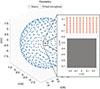 |
Figure 3. The simulation setup used in the current study. 501 point sources on the surface of a sphere with a radius of 10 m generate the diffuse sound field, which is estimated on the 10 × 10 virtual microphone grid shown in red, from the responses of monitoring microphones confined in the grey area. |
To enable comparison with previous studies focusing on arrays exploiting pressure and pressure gradient information [4, 9, 29], the inter-microphone spacing of the monitoring arrays is constrained to approximately 0.0354 m. Moreover, the NMSE at any virtual microphone position is constrained to −30 dB to prevent the GA from over-optimising at a single virtual microphone to achieve high fitness [29].
For each simulation described in the following subsections, 100 independent trials were performed. The global Pareto set has been constructed by merging the Pareto sets from each trial and extracting the non-dominated set. The TOPSIS solutions are calculated from this global Pareto set. To minimise numerical errors without significantly affecting the accuracy of the optimal observation filters, the parameter n in equation (7) is set to 10−6.
5.2 Single frequency optimisation
Initially, the optimisation was performed at a single frequency of 1 kHz. The metrics of equations (8) and (6) have been combined to form the fitness function
 (21)
(21)
where f = 1 kHz. The global Pareto set in this case, calculated from the Pareto sets of 100 trials, is shown in Figure 4, where the solution with the smallest estimation error in the previous preliminary study [29], and the TOPSIS optimal solution, are included for comparison. The shape of the Pareto curve illustrates the difficulty of increasing estimation performance beyond a certain value without significantly increasing the condition number. Although the solution calculated with the Single Objective Optimisation (SOO) [29] is not included in the Pareto set, it lies very close to it. The TOPSIS solution provides a good balance between estimation performance and the conditioning of the PSD matrix.
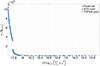 |
Figure 4. The global Pareto set calculated from the Pareto sets of 100 trials for the minimisation of the estimation error and condition number at a single frequency of 1 kHz. The best SOO point and the TOPSIS optimal point are also shown. |
The microphone configurations and the spatial error distribution for the solutions with the minimum estimation error, the TOPSIS optimal solution, the solution with the minimum condition number, and the SOO optimal configuration are shown in Figure 5. From these results it can be seen that the SOO optimal configuration is very similar to the MOO configuration with the minimum performance in the error objective. The minimum error objective is achieved utilising linear arrays pointing towards the centre of the virtual microphone grid. Similar configurations have been investigated in past studies [3, 8] and were found to be sensitive to uncertainties [1, 4, 46], as is also indicated here by the high condition number corresponding to these configurations. In both cases, the spatial distribution of the error has a region of low error at the centre of the first row of virtual microphones close to the monitoring microphone array, with the performance then decreasing at the virtual microphones moving away from this location.
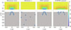 |
Figure 5. The estimation error at the virtual microphones and the corresponding array configurations that achieve the minimum error performance, minimum condition number, and the SOO and TOPSIS optimal configurations. The grey squares mark the permissible region for monitoring microphone placement. |
The minimum in the condition number objective is achieved with a configuration consisting of widely spaced microphones. The microphones are arranged such that the product k r, with k the wavenumber and r the inter-element distance between microphone pairs, approaches the zeros of the sinc(k r) = sin(k r)/k r function, which describes the pressure correlation between positions in a diffuse sound field [47]. The large inter-element distance compared to the excitation wavelength results in highly uncorrelated signals [6, 47], minimising the condition number of Smm. However, the large distance between the microphones and the estimation area results in low multiple coherence between the monitoring and virtual microphones, leading to a limited performance in terms of the estimation error [6] and this can be clearly seen from the spatial error distribution plot in Figure 5.
The TOPSIS optimal solution provides a configuration that balances the error and conditioning objectives. In this case, it can be seen from Figure 5 that the configuration does not have a uniform structure, like in the minimum error case; the microphones are positioned closer to the virtual microphone grid and have a larger spread along the horizontal axis. The lateral extension creates a wider area where the estimation performance is close to −10 dB, compared to the minimum error configuration. However, the minimum error over the virtual microphone grid is higher, and the estimation error increases faster as the distance from the microphone array increases, compared to the minimum error configuration.
5.3 Aggregate multi-frequency optimisation
The optimisation in Section 5.2 is performed for a single frequency, but VS is seldom employed in single-frequency control systems. The approach can be directly extended to multiple frequencies by stacking the scalar metrics of equations (9) and (11) in a vector to form the fitness function
 (22)
(22)
where in this work the three frequencies are f1 = 250 Hz, f2 = 500 Hz, and f3 = 1 kHz.
Figure 6 displays the global Pareto set calculated from 100 independent optimisation trials. As also observed in the single frequency optimisation, improving overall estimation performance beyond a certain point results in a rapid increase in the corresponding condition number. However, in this multi-frequency case, the condition number and estimation error acquire larger values, owing to the aggregated performance over multiple frequencies. The condition number is high due to the significant correlation between the microphone responses at low frequencies [4, 6, 7, 47], and the estimation error is larger due to the accumulated errors over frequency in the metric.
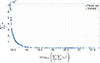 |
Figure 6. The global Pareto set calculated from the Pareto sets of 100 trials for the minimisation of the sum of the estimation error and condition number over the frequencies of 250 Hz, 500 Hz, and 1 kHz. The TOPSIS optimal point is also shown. |
The spatial distribution of the estimation error over the virtual microphones for the microphone configurations that minimise the error, the condition, and the TOPSIS optimal setup are shown in Figure 7 at the three considered frequencies along with the microphone array geometries. The minimum error configuration forms a curved array close to the virtual microphone estimation area. The curvature enables the exploitation of pressure gradient components along multiple directions to be utilised in the estimation process [4, 8] while keeping the monitoring microphones close to the virtual microphone positions, maximising the potential coherence [6, 19]. A circular sub-array on one side provides uniform spatial extension for the area where good estimation is achieved, which is particularly beneficial at low and mid frequencies. The estimation error is consistently below −10 dB over the entire virtual microphone grid at 250 Hz and becomes increasingly localised close to the microphone configuration with increasing frequency. The spatial distribution of the estimation error at 1 kHz is similar to the single frequency TOPSIS configuration. Notably, this minimum error configuration closely matches the configuration that achieved one of the lowest error fitness scores in the preliminary study [29], despite an SOO optimisation being performed only at 1 kHz.
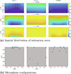 |
Figure 7. The (a) spatial distribution of the estimation error and (b) the corresponding microphone configurations that minimise the error, condition, and the TOPSIS optimal setup calculated with the J2 fitness function over the frequencies of 250 Hz, 500 Hz, and 1 kHz. The grey squares mark the permissible region for monitoring microphone placement. |
For the configuration that minimises the condition number, it can be seen from Figure 7 that optimal performance is achieved by maximising the average inter-element spacing, with a widely spaced and pseudo-random distribution. The large distance between the monitoring and virtual microphones in this case degrades coherence and reduces the estimation accuracy [6]. At the frequency of 250 Hz, the largest estimation error remains below −10 dB; however, at higher frequencies it is consistently above that threshold over the entire microphone grid.
Finally, the TOPSIS selected configuration resembles the minimum error configuration when the condition number is constrained to κ ≤ 103, in the preliminary study [29]. It consists of two linear sub-arrays directed towards the estimation zone, positioned on each side of a pair also orientated towards the virtual microphones. As observed in the single frequency optimisation, aligning the sub-arrays toward a common focal point in the estimation region improves high-frequency estimation performance, while their lateral spread reduces the condition number of the configuration and broadens the region of improved estimation along the horizontal axis. The estimation performance at low and mid frequencies is similar to that of the minimum error configuration, with the lateral extension of the area at which the error is below −10 dB being slightly smaller in the TOPSIS configuration case. At 1 kHz the performance of the TOPSIS configuration decreases, and the error is higher than −10 dB at all virtual microphone locations.
It is common for GA algorithms minimising weighted sum fitness functions, such as equations (9) and (11), to focus on the term of the function whose weighted magnitude is the largest [43]. For example, for the error objective in the fitness function J2, this would be the error at the lowest frequency, as this is the easiest to minimise, the one that acquires the largest, in absolute value, magnitude, and the errors are equally weighted for all frequencies. However, this behaviour is not observed here with the minimum error optimal solution exhibiting average performance across all frequencies (see Tab. 1 in Sect. 5.5). The constraint of the error being at best −30 dB at each virtual microphone provides a safeguard forcing the algorithm to search for solutions that achieve good estimation performance at all frequencies in order to provide a significant fitness score improvement.
5.4 Multi-frequency optimisation
In this section, rather than solving the multi-frequency optimisation using the error and conditioning metric averaged over the considered frequencies, the individual frequency metrics given by equations (8) and (6) can be directly combined to form a fitness vector. In this case, two fitness functions are defined. The first function is defined for the estimation error minimisation, which incorporates equation (8) evaluated at the three frequencies, to give
 (23)
(23)
and the second fitness function augments equation (21) with the condition number provided by equation (6) evaluated at the same three frequencies
 (24)
(24)
Because the global Pareto fronts are assembled from the Pareto sets of individual trials, the fronts acquired with the two fitness functions contain different number of points. However, visualising these sets is difficult due to the dimensionality of the fitness functions. The minimum error solution is consistently calculated with the J3 function for all frequencies, with the J4 minimum error solutions exhibiting larger condition numbers than their J3 counterparts; however, both configurations have very high condition numbers, rendering the numerical differences between them of minimal practical significance (see Tab. 1 in Sect. 5.5). Solutions obtained with J4 minimisation represent configurations that optimally compromise between estimation performance and robustness to uncertainties; a trade-off that can be calculated only if the condition is introduced in the fitness function.
Figure 8 displays the configurations that minimise the fitness function objectives at each frequency, along with the two TOPSIS optimal solutions. Notably, the configurations that minimise the estimation error at 1 kHz are nearly identical for both fitness functions and match those obtained via both SOO and MOO at a single frequency. As with the optimal arrays at 1 kHz, the arrays minimising the error at the other two frequencies consist of linear sub-arrays whose axes are orientated towards the estimation area, extending the region over which significant estimation performance gains are achieved [4, 9]. However, unlike the 1 kHz case, these sub-arrays are not focused on a single point; instead, their axes diverge to provide broader spatial coverage. Moreover, a line of three monitoring microphones arranged as close as possible to the virtual microphones offers high estimation accuracy near the configuration, owing to the high coherence at these frequencies [6]. At 250 Hz, the configurations include a single microphone optimally positioned at the intersection of the linear sub-array axes, enhancing the estimation extension along both arrays. At 500 Hz, to preserve the estimation gains provided by linear microphone arrangements, the configurations become denser relative to those at 250 Hz, since the wavelength has now been halved [7]. The microphone at the intersection of the sub-array axes remains in the configuration stemming from the J3 function, resulting in a more symmetric spatial error distribution compared to that calculated from J4. Progressing from 500 Hz to 1 kHz, where the wavelength is again halved, a similar inter-element spacing reduction is observed. The minimum error configurations calculated with this multi-frequency approach are optimised for each frequency and achieve better estimation performance than the corresponding configuration calculated for the average of the frequencies.
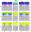 |
Figure 8. Spatial estimation error distribution over the virtual microphone grid for the configurations minimising the objectives of the fitness functions J3 and J4 and the two TOPSIS optimal solutions. The grey squares mark the permissible region for monitoring microphone placement. |
It can also be seen from Figure 8 that condition number minimisation is achieved by increasing the spacing between monitoring microphones so that their responses become less correlated, as was also observed in the preceding optimisation cases. However, in this case, a single configuration achieves the lowest condition number at both 250 Hz and 500 Hz, whereas a different configuration is optimal at the frequency of 1 kHz. At 1 kHz, the configuration that minimises the condition number closely resembles that calculated with MOO at 1 kHz rotated by 180°. Positioning the microphones such that the k r values result in zero correlation between the microphones, as in the 1 kHz configuration, is not feasible at the two lower frequencies, due to the limited available space. Consistent with earlier findings, all configurations that minimise the condition number exhibit poor estimation performance because the microphones are positioned far from the estimation region, leading to low coherence between the monitoring and virtual microphones [3, 6].
The TOPSIS solutions shown in Figure 8 provide a compromise by balancing performance across the three frequencies for the J3 function and by jointly considering performance and condition number for the J4 function. Both TOPSIS configurations resemble the corresponding optimal layouts at 250 Hz and 500 Hz more closely than the 1 kHz solution. The J3 configuration forms a triangular array, similar to the optimal solution at 250 Hz, whereas the J4 configuration is nearly rectangular. Each setup includes three microphones on the line nearest the virtual microphone grid, with a pair of microphones positioned behind them to form a two-element diverging linear array directed toward the estimation region, introducing pressure gradient information in the estimation process [4, 7–9]. The remaining three microphones are positioned further back within the monitoring region, extending the linear arrays. In the J4 configuration, these microphones are spaced more widely than in the J3 solution, to control the PSD matrix condition.
5.5 Comparative evaluation of optimal solutions
Throughout this study, different optimisation approaches have been shown to provide distinct optimal configurations with varying performance and robustness characteristics. In this section, the performance and robustness of the optimal configurations obtained in Sections 5.2–5.4 are evaluated over a broad frequency range, and the observed similarities and differences are evaluated and related to the underlying physical microphone topologies.
Table 1 summarises the NMSE and condition number for the minimum error and TOPSIS configurations derived from the four fitness functions, J1–J4, and the minimum condition configuration calculated with J4, at the three optimisation frequencies. Across all frequencies, the minimum NMSE formulations achieve the smallest errors; J3 yields the lowest NMSE because it minimises the error without being affected by the conditioning of the configurations. The J1 minimum NMSE solution is optimal at its design frequency of 1 kHz, but performs comparatively poorly at the other two frequencies. The J2 configuration improves slightly on J1 at low and mid frequencies, but the gain in the conditioning is marginal, except at 1 kHz. As discussed previously, J3 and J4 produce very similar minimum error results, with J4 exhibiting slightly higher NMSE, with higher condition numbers. At 250 Hz, the NMSE values span approximately 10 dB, but this spread narrows considerably as the frequency increases to 500 Hz, and becomes negligible at 1 kHz, indicating that the choice of fitness function has a diminishing influence on the spatially summed NMSE at higher frequencies. TOPSIS configurations consistently exhibit lower estimation performance, but the range of NMSE values among them is smaller.
Estimation error and condition number for the solutions calculated by minimising J1, J2, J3 and J4.
Condition numbers differ by several orders of magnitude. For the minimum NMSE solutions, the condition numbers are very large at 250 Hz and 500 Hz and, although a reduction is observed at 1 kHz, the condition remains large. In contrast, TOPSIS solutions exhibit a significant reduction in condition number. Particularly, the J2 TOPSIS configuration achieves the smallest condition number, at least one order of magnitude smaller than most other setups, excluding the minimum norm solution. This demonstrates that TOPSIS selection can substantially improve numerical stability while incurring only a modest increase in NMSE.
Overall, the minimum NMSE solutions achieve the lowest error, but suffer from poorly conditioned PSD matrices, whereas the TOPSIS solutions offer a balanced compromise; a slight increase in NMSE coupled with markedly lower condition numbers, which can be advantageous for practical implementations of an RMT VS system [3, 5].
Figure 9 presents the average NMSE, its range, and the condition number of the minimum error and TOPSIS configurations in Table 1 over the frequency range [100 Hz,1.5 kHz]. The average performance is consistent across all configurations. Small deviations are evident between the optimal and TOPSIS solutions for J1 and J2, while for J3 and J4 the main differences in the mean occur between the high frequency minimum error solution and the remaining configurations at frequencies below approximately 400 Hz.
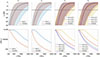 |
Figure 9. Estimation error and condition number of the monitoring microphone PSD matrix for the minimum NMSE and TOPSIS solutions calculated by optimising the fitness functions J1–J4, over the frequency range [100 Hz,1.5 kHz]. |
The J1 and J2 configurations maintain NMSE better than −10 dB over the entire estimation area up to about 350 Hz, whereas J3 and J4 configurations extend this range up to roughly 400 Hz. However, the frequency at which the NMSE is below −10 dB at least at one virtual microphone location varies significantly across different setups. From Figures 5, 7–9, it can be seen that dense configurations shift this threshold higher in frequency, but at the cost of reduced robustness, as reflected in the larger condition numbers. Except for the J3 minimum NMSE solution for the 250 Hz, TOPSIS configurations exhibit the lowest such threshold for the −10 dB NMSE criterion, reflecting the trade-off between performance and robustness. Notably, the condition number correlates well with the frequency limit at which the −10 dB NMSE limit is crossed, reinforcing the inverse relation between numerical robustness and broadband estimation accuracy [3–5, 32].
6 Conclusions
This article has presented an investigation into the application of a GA to calculate optimal microphone configurations for estimating the pressure in a stationary diffuse sound field with the RMT VS method. Multi-objective optimisation was performed using several fitness functions that combine the estimation error and the condition number of the monitoring microphone PSD matrix, thereby addressing both performance and robustness. Optimisations were performed for a simulated tonal diffuse field at a single frequency and at three frequencies spanning three octaves.
The TOPSIS decision-making method was applied to select a single configuration that provides a balanced trade-off between the objectives forming each fitness function. The resulting optimal and TOPSIS solutions were evaluated at the optimisation frequencies, and their physical topologies were examined to identify patterns that promote the optimality criteria. The study reveals that linear configurations pointing towards the estimation region improve estimation performance. Two distinct approaches to minimise estimation error were identified. At low and mid frequencies, diverging linear sub-arrays increased the coherence between the monitoring configuration and the virtual microphones [4, 6, 9]. At higher frequencies, increasing the estimation is achieved by focusing linear sub-arrays on a single virtual microphone close to the configuration.
Consistent with previous work [4, 48], dense configurations that incorporate pressure gradient information provide performance gains but exhibit high condition numbers, reducing robustness to uncertainties. Configurations that minimise the condition number achieved optimal results at low and mid frequencies by increasing inter-element spacing; at high frequencies, optimal placement results in the product of inter-element distances and wavenumber approaching the value for which the pressure correlation in a diffuse field becomes zero [6, 47]. This distance does not necessarily correspond to the maximum possible spacing. However, large spacings significantly reduced the coherence between monitoring and virtual microphones, leading to very poor overall performance. Incorporating the condition number into the fitness function slightly raised the estimation error without reducing the condition number of these configurations. In contrast, TOPSIS solutions offered a favourable trade-off, providing modest increases in estimation error while achieving condition numbers an order of magnitude lower than those of the minimum-error designs.
Both the minimum error and TOPSIS configurations were assessed over a broad frequency range. Their average estimation performances were found to be comparable. Optimisation strategies focusing solely on minimising the estimation error achieved the best estimation performance, but resulted in poorly conditioned configurations. All configurations achieved at most −10 dB estimation error across the entire estimation region up to approximately 350 Hz. The condition number exhibited a positive correlation with the frequency at which the estimation error exceeds −10 dB over the entire estimation area; denser microphone layouts extended this limit to higher frequencies at the expense of higher condition numbers, highlighting the inverse relationship between robustness and estimation accuracy [4, 48].
Estimation performance is governed by the coherence between monitoring and virtual microphone positions [6]. The findings of the current work reinforce earlier studies [4, 8, 9] focusing on the use of arrays incorporating pressure gradient information in the estimation process to increase the coherence between monitoring and virtual microphones. While the present work focused on optimal configurations for the estimation of a diffuse sound field, prior investigations [3, 5, 9, 11] have shown that the performance and robustness of the RMT vary across different acoustic environments. Directional sound field components exhibit high coherence between positions along the propagation direction [3, 9], whereas modal fields can give rise to observability issues [49, 50]. The arrays calculated in the current study exploit pressure gradient along multiple directions and feature non-uniform geometries, which can improve performance compared to certain uniform configurations in some types of sound fields, such as, for example, a linear array placed near or along nodal lines in a modal field. However, the optimality of the presented arrays is not guaranteed for all types of sound fields, and further research is required to identify globally optimal design patterns across diverse acoustic environments.
Acknowledgments
The authors would like to acknowledge the use of the IRIDIS High Performance Computing Facility and associated support services at the University of Southampton in the completion of this work.
Funding
This work was supported by the project “IN-NOVA: Active reduction of noise transmitted into and from enclosures through encapsulated structures,” which has received funding from the European Union’s Horizon Europe programme under the Marie Skłodowska-Curie Grant No. 101073037 and by the UK Research and Innovation under the UK government’s Horizon Europe funding agreement with Grant No. EP/X027767/1. J.C. was supported by the Department of Science, Innovation and Technology (DSIT) Royal Academy of Engineering under the Research Chairs and Senior Research Fellowships programme.
Conflict of interest
The authors have no conflicts to disclose.
Data availability statement
Data are available on request from the authors.
Author contribution statement
Achilles Kappis: Conceptualisation, methodology, software, visualisation, writing – original draft, writing – review & editing. Jordan Cheer: Methodology, resources, writing – review & editing, supervision, project administration, funding acquisition.
References
- D. Moreau, B. Cazzolato, A. Zander, C. Petersen: A review of virtual sensing algorithms for active noise control. Algorithms 1 (2008) 69–99. [CrossRef] [Google Scholar]
- M. Pawelczyk: Adaptive noise control algorithms for active headrest system. Control Engineering Practice 12 (2004) 1101–1112. [Google Scholar]
- W. Jung, S.J. Elliott, J. Cheer: Estimation of the pressure at a listener’s ears in an active headrest system using the remote microphone technique. Journal of the Acoustical Society of America 143 (2018) 2858–2869. [Google Scholar]
- A. Kappis, J.A. Zhang, J. Cheer: Remote microphone virtual sensing with nested microphone sub-arrays. Journal of the Acoustical Society of America 158 (2025) 407–418. [Google Scholar]
- J. Zhang, S.J. Elliott, J. Cheer: Robust performance of virtual sensing methods for active noise control. Mechanical Systems and Signal Processing 152 (2021) 107453. [CrossRef] [Google Scholar]
- P. Zhang, S. Wang, H. Duan, J. Tao, H. Zou, X. Qiu: A study on coherence between virtual signal and physical signals in remote acoustic sensing. Journal of the Acoustical Society of America 152 (1) (2022) 2840–2848. [Google Scholar]
- S. Elliott, J. Garcia-Bonito: Active cancellation of pressure and pressure gradient in a diffuse sound field. Journal of Sound and Vibration 186 (1995) 696–704. [Google Scholar]
- D.J. Moreau, J. Ghan, B.S. Cazzolato, A.C. Zander: Active noise control in a pure tone diffuse sound field using virtual sensing. Journal of the Acoustical Society of America 125 (2009) 3742–3755. [CrossRef] [PubMed] [Google Scholar]
- H. Li, S. Wang, J. Tao, X. Qiu: Enhancing the coherence between virtual and physical signals in virtual sensing with a double-layer microphone arrangement. Journal of the Acoustical Society of America 157 (2025) 2392–2403. [Google Scholar]
- B.S. Cazzolato, J. Ghan: Frequency domain expressions for the estimation of time-averaged acoustic energy density. Journal of the Acoustical Society of America 117 (2005) 3750–3756. [Google Scholar]
- W. Jung, S.J. Elliott, J. Cheer: Local active control of road noise inside a vehicle. Mechanical Systems and Signal Processing 121 (2019) 144–157. [CrossRef] [Google Scholar]
- A. Krause, A. Singh, C. Guestrin: Near-optimal sensor placements in Gaussian processes: theory, efficient algorithms and empirical studies. Journal of Machine Learning Research 9 (2008) 235–284. [Google Scholar]
- K. Ariga, T. Nishida, S. Koyama, N. Ueno, H. Saruwatari: Mutual-information-based sensor placement for spatial sound field recording, in: Proceedings of the IEEE International Conference on Acoustics, Speech, Signal Process. (ICASSP), Barcelona, Spain, May, 2020, pp. 166–170. [Google Scholar]
- N. Ueno, S. Koyama, H. Saruwatari: Kernel ridge regression with constraint of the Helmholtz equation for sound field interpolation, in: Proceedings of the IEEE International Workshop on Acoustic Signal Enhancement (IWAENC), Tokyo, 2018, pp. 1–440. [Google Scholar]
- G. Chardon, W. Kreuzer, M. Noisternig: Design of spatial microphone arrays for sound field interpolation. IEEE Journal of Selected Topics in Signal Processing 9, 5 (2015) 780–790. [Google Scholar]
- M. Barrault, Y. Maday, N.C. Nguyen, A.T. Patera: An ‘empirical interpolation’ method: application to efficient reduced-basis discretization of partial differential equations. Comptes Rendus Mathematique 339, 9 (2004) 667–672. [Google Scholar]
- S. Koyama, G. Chardon, L. Daudet: Joint source and sensor placement for sound field control based on empirical interpolation method, in: Proceedings of the IEEE International Conference on Acoustics, Speech, Signal Process. (ICASSP) Calgary, AB, 2018, pp. 501–505. [Google Scholar]
- S. Koyama, G. Chardon, L. Daudet: Optimizing source and sensor placement for sound field control: an overview. IEEE/ACM Transactions on Audio, Speech, and Language Processing 28 (2020) 696–714. [Google Scholar]
- S.A. Verburg, F. Elvander, T. Van Waterschoot, E. Fernandez-Grande: Optimal sensor placement for the spatial reconstruction of sound fields. EURASIP Journal on Audio, Speech, and Music Processing 2024 (2024) 41. [Google Scholar]
- S. Katoch, S.S. Chauhan, V. Kumar: A review on genetic algorithm: past, present, and future. Multimedia Tools and Applications 80 (2021) 8091–8126. [CrossRef] [Google Scholar]
- F. Neri, C. Cotta, P. Moscato, J. Kacprzyk, Eds.: Handbook of Memetic Algorithms. Studies in Computational Intelligence. Vol. 379. Springer, Berlin, Heidelberg, 2012. [Google Scholar]
- D.C. Zimmerman: A Darwinian approach to the actuator number and placement problem with non-negligible actuator mass. Mechanical Systems and Signal Processing 7 (1993) 363–374. [Google Scholar]
- S. Katsikas: A genetic algorithm for active noise control actuator positioning. Mechanical Systems and Signal Processing 9 (1995) 697–705. [Google Scholar]
- S. Wrona, M. Pawelczyk: Shaping frequency response of a vibrating plate for passive and active control applications by simultaneous optimization of arrangement of additional masses and ribs. Part II: optimization. Mechanical Systems and Signal Processing 70–71 (2016) 699–713. [Google Scholar]
- S. Wrona, M. Pawelczyk, J. Cheer: Acoustic radiation-based optimization of the placement of actuators for active control of noise transmitted through plates. Mechanical Systems and Signal Processing 147 (2021) 107009. [Google Scholar]
- S. Wrona, M. De Diego, M. Pawelczyk: Shaping zones of quiet in a large enclosure generated by an active noise control system. Control Engineering Practice 80 (2018) 1–16. [Google Scholar]
- X. Zheng, Z. Jia, B. Wan, M. Zeng, Y. Qiu: A study on hybrid active noise control system combined with remote microphone technique. Applied Acoustics 205 (2023) 109296. [Google Scholar]
- K. Deb: Multi-objective optimization using evolutionary algorithms: an introduction. Technical Report 2011003, Indian Institute of Technology Kanpur, 2011. [Google Scholar]
- A. Kappis, J. Cheer: Topology optimisation of microphone arrays for remote microphone virtual sensing in diffuse sound fields, in: Proceedings of the 11th Convention of the European Acoustics Association, Forum Acusticum/EuroNoise 2025, Málaga, Spain, 2025. [Google Scholar]
- L. Zadeh: Optimality and non-scalar-valued performance criteria. IEEE Transactions on Automatic Control 8 (1963) 59–60. [Google Scholar]
- S.J. Elliott, J. Cheer: Modeling local active sound control with remote sensors in spatially random pressure fields. Journal of the Acoustical Society of America 137 (2015) 1936–1946. [Google Scholar]
- S.J. Elliott, J. Cheer, J.-W. Choi, Y. Kim: Robustness and regularization of personal audio systems. IEEE Transactions on Audio, Speech and Language Processing 20 (2012) 2123–2133. [Google Scholar]
- W. Jung, S.J. Elliott, J. Cheer: Combining the remote microphone technique with head-tracking for local active sound control. Journal of the Acoustical Society of America 142 (2017) 298–307. [Google Scholar]
- Y. Censor: Pareto optimality in multiobjective problems. Applied Mathematics & Optimization 4 (1977) 41–59. [Google Scholar]
- MathWorks: gamultiobj MATLAB Help Center, 2025. [Google Scholar]
- K. Deb: An efficient constraint handling method for genetic algorithms. Computer Methods in Applied Mechanics and Engineering 186 (2000) 311–338. [Google Scholar]
- B.L. Miller, D.E. Goldberg: Genetic algorithms, tournament selection, and the effects of noise. Complex Systems 9 (1995) 193–212. [MathSciNet] [Google Scholar]
- G. Pavai, T.V. Geetha: A survey on crossover operators. ACM Computing Surveys 49 (2017) 1–43. [Google Scholar]
- K. Deb: Simulated binary crossover for continuous search space. Complex Systems 9 (1995) 115–148. [Google Scholar]
- K. Deb, D. Deb: Analyzing mutation schemes for real-parameter genetic algorithms. Technical Report 2012016, Indian Institute of Technology Kanpur. [Google Scholar]
- C.-L. Hwang, K. Yoon: Multiple Attribute Decision Making. Lecture Notes in Economics and Mathematical Systems. Vol. 186. Springer, Berlin, Heidelberg, 1981. [Google Scholar]
- N. Vafaei, R.A. Ribeiro, L.M. Camarinha-Matos: Normalization techniques for multi-criteria decision making: analytical hierarchy process case study, in: L.M. Camarinha-Matos et al., Eds. Technological Innovation for Cyber-Physical Systems. Vol. 470. Springer International Publishing, Cham, 2016, pp. 261–269. [Google Scholar]
- R.T. Marler, J.S. Arora: The weighted sum method for multi-objective optimization: new insights. Structural and Multidisciplinary Optimization 41, 6 (2010) 853–862. [Google Scholar]
- A. González: Measurement of areas on a sphere using Fibonacci and latitude-longitude lattices. Mathematical Geosciences 42 (2010) 49–64. [Google Scholar]
- F. Zotter, S. Riedel, L. Gölles, M. Frank: Diffuse sound field synthesis: ideal source layers. Acta Acustica 8 (2024) 34. [Google Scholar]
- J.M. Munn, B.S. Cazzolato, C.H. Hansen, C.D. Kestell: Higher-order virtual sensing for remote active noise control, 2002. [Google Scholar]
- F. Jacobsen: The diffuse sound field - statistical considerations concerning the reverberant field in the steady state. Technical Report 27, Technical University of Denmark, 1979. [Google Scholar]
- C.D. Kestell, B.S. Cazzolato, C.H. Hansen: Active noise control in a free field with virtual sensors. Journal of the Acoustical Society of America 109 (2001) 232–243. [Google Scholar]
- Y.C. Park, S.D. Sommerfeldt: Global attenuation of broadband noise fields using energy density control. Journal of the Acoustical Society of America 101, 1 (1997) 350–359. [Google Scholar]
- J.W. Parkins, S.D. Sommerfeldt, J. Tichy: Narrowband and broadband active control in an enclosure using the acoustic energy density. Journal of the Acoustical Society of America 108, 1 (2000) 192–203. [Google Scholar]
Cite this article as: Kappis A. & Cheer J. 2026. Optimisation of the spatial configuration of microphones for robust virtual sensing in a diffuse sound field. Acta Acustica, 10, 22. https://doi.org/10.1051/aacus/2026018.
All Tables
Estimation error and condition number for the solutions calculated by minimising J1, J2, J3 and J4.
All Figures
|
Figure 1. Block diagram of a remote microphone virtual sensing system. An observation filter, |
| In the text | |
|
Figure 2. The logic diagram of a genetic algorithm. A random initial population is generated and its individuals are crossed over and mutated to create a new generation. When a stop criterion is met, the optimisation is terminated. |
| In the text | |
|
Figure 3. The simulation setup used in the current study. 501 point sources on the surface of a sphere with a radius of 10 m generate the diffuse sound field, which is estimated on the 10 × 10 virtual microphone grid shown in red, from the responses of monitoring microphones confined in the grey area. |
| In the text | |
|
Figure 4. The global Pareto set calculated from the Pareto sets of 100 trials for the minimisation of the estimation error and condition number at a single frequency of 1 kHz. The best SOO point and the TOPSIS optimal point are also shown. |
| In the text | |
|
Figure 5. The estimation error at the virtual microphones and the corresponding array configurations that achieve the minimum error performance, minimum condition number, and the SOO and TOPSIS optimal configurations. The grey squares mark the permissible region for monitoring microphone placement. |
| In the text | |
|
Figure 6. The global Pareto set calculated from the Pareto sets of 100 trials for the minimisation of the sum of the estimation error and condition number over the frequencies of 250 Hz, 500 Hz, and 1 kHz. The TOPSIS optimal point is also shown. |
| In the text | |
|
Figure 7. The (a) spatial distribution of the estimation error and (b) the corresponding microphone configurations that minimise the error, condition, and the TOPSIS optimal setup calculated with the J2 fitness function over the frequencies of 250 Hz, 500 Hz, and 1 kHz. The grey squares mark the permissible region for monitoring microphone placement. |
| In the text | |
|
Figure 8. Spatial estimation error distribution over the virtual microphone grid for the configurations minimising the objectives of the fitness functions J3 and J4 and the two TOPSIS optimal solutions. The grey squares mark the permissible region for monitoring microphone placement. |
| In the text | |
|
Figure 9. Estimation error and condition number of the monitoring microphone PSD matrix for the minimum NMSE and TOPSIS solutions calculated by optimising the fitness functions J1–J4, over the frequency range [100 Hz,1.5 kHz]. |
| In the text | |
Current usage metrics show cumulative count of Article Views (full-text article views including HTML views, PDF and ePub downloads, according to the available data) and Abstracts Views on Vision4Press platform.
Data correspond to usage on the plateform after 2015. The current usage metrics is available 48-96 hours after online publication and is updated daily on week days.
Initial download of the metrics may take a while.