| Issue |
Acta Acust.
Volume 10, 2026
|
|
|---|---|---|
| Article Number | 23 | |
| Number of page(s) | 17 | |
| Section | Hearing, Audiology and Psychoacoustics | |
| DOI | https://doi.org/10.1051/aacus/2026019 | |
| Published online | 03 April 2026 | |
Scientific Article
The effect of vehicle sound power on auditory time-to-collision estimation
1
Johannes Gutenberg-Universität Mainz, Psychologisches Institut, Section Experimental Psychology, Mainz
Germany
2
Rice University, Department of Psychological Sciences, Houston
Texas
USA
* Corresponding author: This email address is being protected from spambots. You need JavaScript enabled to view it.
Received:
11
June
2025
Accepted:
18
February
2026
Abstract
To safely cross a street while a vehicle is approaching, pedestrians must estimate how long it will take for the vehicle to reach their position. Recent studies have shown that estimation of a vehicle’s arrival time (i.e., time-to-collision (TTC) estimation) is affected by the intensity of the vehicle’s sound. When presented with the same actual TTC, louder sound sources were perceived as arriving earlier than quieter sources (the so-called “intensity-arrival effect”). However, in these experiments the vehicle sound power (also referred to as source intensity) was varied from trial to trial, potentially directing participants’ attention to the intensity variation. Here, we used high fidelity acoustic simulations of approaching vehicles, to investigate whether the effect of vehicle sound power on auditory TTC estimation persists when it is varied from block to block rather than from trial to trial. Results showed a significant intensity-arrival effect for the blockwise vehicle sound power variation. However, this effect was much weaker compared to a condition where the vehicle sound power varied from trial to trial.
Key words: Time-to-contact estimation / Pedestrian safety / Auditory perception / Virtual acoustics / Intensity-arrival effect / Vehicle sound power
© The Author(s), Published by EDP Sciences, 2026
 This is an Open Access article distributed under the terms of the Creative Commons Attribution License (https://creativecommons.org/licenses/by/4.0), which permits unrestricted use, distribution, and reproduction in any medium, provided the original work is properly cited.
1 Introduction
Accurate perception of the motion of vehicles is vital for safe pedestrian-vehicle interactions. When crossing a street while a vehicle is approaching, pedestrians must (a) estimate how long it will take for the vehicle to reach their position, and (b) judge whether this time is long enough to cross the road safely in front of the vehicle, or whether they should wait until the vehicle has passed them. Recent studies have shown evidence of an “intensity arrival effect” [1], an auditory analog of the “size-arrival effect” [2] that is one of the most prominent characteristics of visual arrival time estimation. The intensity-arrival effect describes that when moving objects with identical arrival times (often denoted as “time-to-collision”; abbreviated as “TTC” hereafter) were presented, participants estimated quieter objects to arrive later at their position than louder objects [1, 3], even when high-fidelity acoustic simulations of approaching vehicles were presented [4, 5], and even when full visual information was available [4, 5]. Such relative overestimations of the arrival times of quieter vehicles appear particularly relevant in light of an increasing number of electric vehicles (EVs) on the road. The EVs typically are quieter than vehicles with internal combustion engine (ICEVs), that is, they have a lower sound power (also referred to as source intensity, e.g., [5]), at least at lower speeds when the contribution of tire noise to the total vehicle noise intensity is relatively weak [6]. The sound power refers to the energy emitted by a sound source per unit time [7]. For a given vehicle, the sound power depends on, for example, the travel speed, engine rotational speed, engine load [6], and also on the road-surface- and tire-characteristics [8, 9]. However, some vehicles (e.g., a small EV) on average produce a lower sound power than other vehicles (e.g., a truck with internal combustion engine). According to vehicle noise measurements and current road traffic noise models, the sound power difference in constant speed pass-by between passenger cars with electric and combustion engine can be 5–15 dB at lower speeds [10–14]. The sound intensity (or sound pressure) at the receiver position (e.g., at the position of the pedestrian in a street-crossing scenario), i.e., the strength of the vehicle sound at the pedestrian’s position, depends on the sound power of the vehicle, but also on the distance between the sound source (vehicle) and the receiver (pedestrian). Due to spherical spreading and air absorption, the sound intensity at the receiver position decreases with increasing distance from the source [7]. When two different vehicles are at the same distance from the receiver, the sound intensity at the receiver position is higher for the vehicle with the higher sound power (assuming identical sound spectra). A visual analogy is the relationship between object size and optical (i.e., retinal) size. Two objects can have different physical sizes, but the optical size, i.e., the visual angle subtended by the object, depends not only on the object’s size, but also on the distance between the object and the observer. For sound frequencies within the audible range, the sound intensity at the receiver position is the major factor determining the perceived intensity of the sound, termed loudness [15].
The visual size-arrival effect in TTC estimation has been suggested as a partial cause for accidents involving motorcycles, e.g., [16–19]. Similarly, the auditory intensity-arrival effect in TTC estimation could play a role in pedestrian or bicyclist accidents involving electric vehicles, which occur disproportionally more often compared to combustion engine vehicles [20–22]. The size-arrival effect has been demonstrated in many configurations, using simple laboratory stimuli or simulated traffic scenarios, different tasks, etc., e.g., [16, 17, 23, 24]. However, it is not fully robust because, for example, object familiarity has been shown to reduce or even fully remove the size-arrival effect [25, 26]. Similarly, the intensity-arrival effect might also be weakened under some conditions. As such, a deeper insight into the conditions in which the intensity-arrival effect occurs is relevant for pedestrian safety. Thus, in the present experiment we evaluated if the type of vehicle sound power variation (between blocks versus between trials) affects the size of the intensity-arrival effect.
In the previous experiments investigating the intensity-arrival effect [1, 3–5], the vehicle sound power varied from trial to trial. Although this situation corresponds to an everyday street-crossing situation where the different approaching vehicles also vary in sound power (e.g., a quieter EV might be followed by a louder ICEV), the trial-to-trial power variation might have directed the participant’s attention to the differences in loudness (i.e., the perceived intensity of the vehicle sound) and thus might have amplified the effect of vehicle sound power on TTC estimation. Even for the size-arrival effect, to our knowledge no work has measured effects of whether relative size varied from trial to trial or between blocks. There are studies where the size was varied between blocks, (e.g., [26]) instead of from trial to trial. However, the difference between the two types of presentations was not measured.
To investigate whether TTC estimation is affected by not only the intensity difference between trials, but also by the “absolute” intensity of an approaching vehicle, we varied the vehicle sound power in a blockwise fashion. We presented acoustic simulations of a vehicle with internal combustion engine approaching a pedestrian at the roadside at three different constant speeds. At each speed, we created a condition with higher vehicle sound power and a condition with lower vehicle sound power by applying an audio gain of either 0 dB (lower) or +10 dB (higher) to the source signals used in the simulation (see Sect. 2.1). We measured the difference in estimated TTC between the blocks presenting only quieter vehicles (i.e., audio gain 0 dB, lower sound power) and blocks presenting only louder vehicles (i.e., audio gain +10 dB, higher sound power). As the comparison condition, we presented blocks in which the vehicle sound power varied from trial to trial (as in the previous studies) and compared the effect of vehicle sound power on the estimated TTCs between the blockwise and trial-to-trial type of sound power variation. Note that, as explained above, the sound power depends on factors such as the travel speed and the road-surface characteristics [8, 9], and also varies somewhat across time, even when a vehicle maintains an almost constant speed. As such, there was variability in vehicle sound power also within the lower and higher vehicle sound power conditions. On average, however, the vehicle sound power was 10 dB higher in the experimental condition with lower vehicle sound power (audio gain 0 dB) than in the condition with higher vehicle sound power. In the following we specifically use the term “vehicle sound power” to refer to the 10-dB experimental variation in sound power via the audio gain.
In the first session of the experiment, the vehicle sound power was varied in a blockwise fashion. For half of the participants, only the lower vehicle sound power condition (0 dB audio gain) was presented in the first block. For the other half, only the higher vehicle sound power (+10 dB audio gain) was presented in the first block. Thus, in this first block of the experiment, the vehicle sound power (audio gain) did not vary within subjects. As a consequence, in block 1, they had no vehicle sound power with which to make a comparison, aside from their everyday familiarity with vehicle noise. In the second session, participants received exactly the same trials as in session 1, but the two vehicle sound powers (i.e., audio gains) were presented in a randomly interleaved fashion, that is, the vehicle sound power varied from trial to trial. All participants received the same order of the type of sound power variation (blockwise followed by trial-to-trial), to ensure that in the very first block of the experiment, participants would not yet have any within-experiment comparison of two different vehicle sound powers. This allowed us to compare the estimated TTCs between the group that started the experiment with a block presenting the lower sound power and the group that started with a block presenting the higher sound power.
Because in a previous experiment [4], the effect of vehicle sound power on TTC estimates was considerably stronger when only auditory but no visual information about the motion of the approaching vehicles was available, we presented auditory-only simulations of the approaching vehicles. We expected an intensity-arrival effect (i.e., longer estimated TTCs for vehicles with lower sound power) to occur when the vehicle sound power varied between blocks but expected the effect to be weaker than for a trial-to-trial power variation.
2 Methods
2.1 Acoustic virtual-reality simulation of approaching vehicles
The simulation system was an improved version of the source-based approach described in Oberfeld et al. [4]. Audio recordings of real vehicles were used as sound sources in the acoustic simulation software TASCAR (Toolbox for Acoustic Scene Creation and Rendering; [27]; http://www.tascar.org/), to produce a physically plausible auditory simulation of moving sound sources in the experimental setting. The source signals were recordings of a gasoline-powered small passenger car (Kia Rio 1.0 T-GDI 120, model year 2019, 1.0 l, 88 kW, 3 cylinders) with manual transmission and Continental summer tires (ContiSportContact 5, 205/45 R17) driving on a straight trajectory on a flat test track, with various velocity profiles (for details concerning the recording setup and example vehicle sound spectra see [4]). Four free field microphones (Roga MI-17), mounted to the chassis of the car (one above each of the front tires, one above the right back tire and one centrally on the engine hood), recorded the vehicle sound during the drive. Synchronously, the GPS position of the car was recorded with high precision (for details see [4]) such that at each time point in the audio signals, the position, speed, and acceleration of the vehicle was known. During the recordings, the driver tried to maintain a constant speed, but the driven speed of course varied slightly across time, as occurs in real traffic scenarios. The four recorded microphone signals were then used as point sources in TASCAR, positioned as shown in Figure 1. On each trial, the motion of the four vehicle sound sources (each playing back one of the recorded microphone signals) in the acoustic scene was simulated in TASCAR. The trajectory was simulated based on the recorded GPS data, with an update time step of 1 ms.
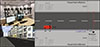 |
Figure 1. The top-left panel shows one of the authors wearing the head-mounted display in the loudspeaker array. The upper ring contains 32 loudspeakers positioned at approximately ear height. The lower ring contains 8 loudspeakers angled up towards the participant. The subwoofer is not visible in the picture. The bottom-left panel shows a screenshot of the visual scene. Note that the approaching vehicle was not presented visually. The right panel shows a bird’s eye view of the simulated scene (to scale). The positions of sources and receiver are indicated in dark gray. The coordinates labelled LF, hood, RF, and RR represent the position of the four vehicle sound sources relative to the center of the front of the car, which played back the sound from the microphones positioned at the left front tire, hood, right front tire, and right rear tire, respectively. |
As shown in Figure 1, the simulated scene was an urban setting with a straight two-lane road and houses along the roadside. In the simulated scene, the left and right house fronts were positioned 15.6 m and 8.4 m from the right curb, respectively. The ground surface and the house fronts were simulated with plausible acoustic reflection properties, based on ISO 9613-2:1999-10 [28]. The reflectance of the floor surface and the house fronts was set, respectively, to ρ = I r /I0 = 1.0 and ρ = 0.8944, where I r is the acoustic intensity of the reflected sound wave and I0 is the intensity of the incoming wave. The sound reflections were modeled with an IIR low pass filter of first order with a cut-off frequency of 5 kHz. Additionally, a first-order Ambisonics recording from a quiet residential area [29] was presented as background noise (LAeq = 37.5 dBA). The simulated receiver in TASCAR was set at the participants position 1 m away from the curb. The height of the receiver was set to match the ear height of the individual participants.
As the simulated vehicle moved through the acoustic scene, TASCAR provided the dynamic processing, for example, continuously updated the position of the vehicle and modeled the distance-dependent change in sound level caused by spherical spreading and air absorption, the distance-dependent sound propagation time (i.e., Doppler shifts were simulated implicitly), and sound reflections from the ground and other surfaces (using an image sound source method; [30]). The resulting dynamic simulations were rendered using sound field synthesis (e.g., [31]). The direct sound and the reflections were rendered separately. For the direct sound, we used 15th order 2D Ambisonics with maxRe decoding [32, 33], played back via 32 Genelec 8020 DPM loudspeakers arranged in a circle with 4.6 m diameter (spaced 11.25 degrees apart), that were positioned around ear height (speaker height 163 cm above the floor) and a subwoofer (Genelec 7360 APM; crossover frequency 62.5 Hz), see the top-left panel in Figure 1. To render the sound reflections from the ground surface and the house fronts, we used 3D vector base amplitude panning (VBAP; [34]) with the full loudspeaker array, containing both the aforementioned 32 loudspeakers at ear height and an additional lower ring of 8 Genelec 8020 DPM speakers (spaced 45 degrees apart and angled towards the listener’s head; ring diameter 4.6 m, speaker height 87 cm above the floor) and the subwoofer. The array was driven by daisy-chained Ferrofish A32 Pro (24-bit audio resolution, fs = 44.1 kHz) and Ferrofish Pulse 16 (24-bit audio resolution, fs = 44.1 kHz) audio converters. The Ferrofish A32 Pro received audio signals via 64-channel MADI from an RME HDSPEe MADI audio interface on a computer running TASCAR under Linux. The 32 loudspeakers of the ear-height ring were driven by the Ferrofish A32 Pro. The 8 loudspeakers of the lower ring and the subwoofer were driven by the Ferrofish Pulse 16.
The loudspeaker array was located on one side of a large lab space (15.00 m × 7.05 m). To reduce interference from acoustic reflections inside the space, the laboratory area containing the loudspeaker array (8.44 m × 7.05 m) was sound-treated. It was separated from the other side of the lab space with sound-absorbing acoustic curtains (Gerriets Bühnenvelours Ascona 570; 570 g/m2; absorption coefficient of 0.95 at frequencies above 400 Hz). A 20 cm thick layer of Basotect G+ (BASF; absorption coefficient of 0.95 at frequencies above 125 Hz) was attached to the walls and ceiling. To reduce reflections from the floor, a carpet (high-pile, IKEA Stoense) was placed inside the array, on top of a 7 mm layer of felt. In addition, 10 cm thick Basotect G+ panels (BASF; absorption coefficient of 0.95 at frequencies above 400 Hz) were added on top of the carpet.
2.2 Visual simulation of the city scene (without vehicles)
In addition to listening to the auditory simulations, participants viewed interactive visual simulations of a city scene (see Fig. 1, bottom left panel), to further their understanding of the spatial layout of the simulated scenario. However, the vehicles were never presented visually, only the surrounding street scenario. Visual simulations were created using the VR-software WorldViz Vizard 7.0 on a Windows computer (Intel Core i9-9900X CPU @ 3.50 GHz, Nvidia Quadro RTX 4000). A Python script controlling the simulation in Vizard also sent commands controlling the corresponding acoustic simulations in TASCAR via the OSC network protocol (https://opensoundcontrol.stanford.edu/).
Participants viewed the virtual visual environment on a head-mounted display (HMD) (HTC Vive Pro Eye). The HMD presented the virtual visual environment stereoscopically via dual OLED displays, each with a diagonal of 3.5′′ and a resolution of 1440 × 1600 pixels per eye (total resolution: 2880 × 1600 pixels, refresh rate: 90 Hz). The field of view of the HMD was 110°. The headphones belonging to the HMD were dismounted for the experiment. Laser-based tracking was used to capture the subject’s head position and orientation in the experimental area. Head and motion tracking transferred the head movements of the participant into the virtual visual environment, so that the participant could move or look around in the simulated visual scene. The participant stood in the center of the loudspeaker array, 1 m away from the right curb in the virtual scene (see Fig. 1). The height of the virtual cameras above the simulated ground surface corresponded to the real eye height of the participant measured by the head tracking.
The visual city scene, based on the Eislebener Straße in Berlin, depicted an urban two-lane road. Vehicles, bicycles, signs etc., were removed from the model, so that the visual scene contained only an asphalt roadway with white markings, the sidewalk including a curb, streetlights and houses. A blue line spanning the width of the street was aligned with the participant’s position in the virtual scene to orient them in the virtual environment. The visually simulated street was approximately 280 m long in the direction from which the car approached and continued 180 m beyond the participant.
2.3 Procedure and design
In an auditory-only condition, a single vehicle with an internal combustion engine (ICEV) approached the participant at different constant velocities (10, 30, 50 km/h). We measured participants’ estimates of the time the front of the vehicle would reach them, that is, their judgments of the vehicle’s time-to-collision (TTC). This was done in a prediction-motion task [35–37]. On each trial, the vehicle sound corresponding to the motion of the approaching vehicle was simulated for a motion duration of 3.0 s, for which we selected a random time interval of 3.0 s from the available recording duration. The available duration varied per recording and was 13, 30 and 7 s for the 10, 30 and 50 km/h recording, respectively. Due to the variations in vehicle speed during a given vehicle recording explained above, the presented motion, sound, and the precise sound power of the car differed slightly from trial to trial for each presented speed (even within conditions that presented the same audio gain), increasing the ecological validity. The acoustic simulation of the motion and the vehicle sound stopped before the vehicle had reached the participant’s position in the virtual scene, as if the sound was blocked completely by an invisible “occluder”. The temporal and spatial distance of the car at “occlusion” (i.e., at the end of the audible part of the approach) was defined by the different simulated TTCs and velocities. Due to the variations in approach speed within drives, the average speed in a 1-s time window before the end of the simulated motion was used for determining the distance at occlusion (Docc) which corresponded to the intended TTC at occlusion (TTCocc). Participants were instructed to pull the trigger of the Vive controller at the exact time when they thought that the vehicle would reach their imaginary crossing path (i.e., the blue line presented in the visual simulation), had the object continued to move towards them with the same velocity as during the audible phase after it was no longer audible. The time interval between the occlusion and the button press was taken as the participant’s estimate of the vehicle’s TTC at the moment of occlusion.
In a factorial design, four parameters were varied within subjects. These included the vehicle’s speed (10, 30, and 50 km/h) and TTC at occlusion (1.25, 2.5, 3.75 and 5.0 s). Each combination of TTC and speed was presented at two different vehicle sound powers (lower, higher), by presenting the audio source signals from the vehicle recordings either at their original amplitude as recorded on the test track (lower, audio gain = 0 dB), or with their increased by 10 dB (higher), by setting the audio gain in the simulation accordingly. In the latter condition, the vehicle sounds can be assumed to having been perceived as approximately two times louder than in the former condition [15]. To put the presented 10-dB power variation into context, note that loudness matches obtained in Oberfeld et al. [4] between the ICEV presented in the present study and an EV (Kia eNiro model year 2019) with deactivated acoustic vehicle alerting system (AVAS; see [38]) showed a 10 dB difference on average at the lowest speed (10 km/h), and differences of 6 dB or less at higher speeds. Pass-by level measurements (Lmax) of ICE passenger vehicles in free flowing traffic on asphalt concrete 0/11 or stone mastic asphalt 0/11 in Germany showed a level variation of approximately 8 dB at a given travel speed (25–80 km/h), in some cases even up to 12–13 dB (see Fig. 6 in [39]). Thus, the 10 dB difference is within the range of vehicle sound level differences that might occur between a quieter vehicle, such as a small EV, and a louder vehicle, such as a large ICEV, at least at a low speed.
We analyzed the A-weighted energy-equivalent sound pressure level at the participant’s position in the last 0.5 s before occlusion (LAeqOcc), which depends not only on the selected vehicle sound power condition (i.e., audio gain), but also on the distance at occlusion and the vehicle speed. For the lower sound power (i.e., audio gain of 0 dB), LAeqOcc ranged from 49.7 to 66.0 dBA across all combinations of speed and TTC at occlusion. For the higher sound power (i.e., audio gain of +10 dB), the LAeqOcc values were of course exactly 10 dB higher (59.7–76.0 dBA).
Participants received the resulting TTC × speed × sound power combinations in two types of vehicle sound power variation (blockwise or trial-to-trial). As depicted in Figure 2, the experiment started with the blockwise sound power variation, followed by a condition with trial-to-trial sound power variation. In the first session, two experimental blocks were presented, and the same vehicle sound power (audio gain) was presented on each trial of a given block. The order of the vehicle sound powers presented in the two blocks of the first session was varied between subjects. Half of the participants started with the block presenting the higher sound power, and the other half started with the lower sound power. In the second session, the vehicle sound power (audio gain) varied from trial to trial. As explained in the introduction, the presentation order of the type of sound power variation was fixed to ensure that in the first block, participants would have no within-experiment vehicle sound power comparison.
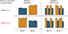 |
Figure 2. Graphical illustration of blocks presented in each session. Bars represent individual trials, and the bar height represents the actual vehicle sound power (including the comparably small variability between trials in the same vehicle sound power condition due to e.g., differing speeds). The orange and blue bars indicate trials presenting the higher (audio gain 10 dB) and lower vehicle sound power (audio gain 0 dB), respectively. All participants started with the blockwise vehicle sound power variation. Half of the participants started with the lower sound power and the other half started with the higher sound power. In the second session, the higher and lower sound powers were presented interleaved (trial-to-trial power variation). |
In a within-subjects design, each participant received all of the 4 (TTC) × 3 (speed) × 2 (vehicle sound power; audio gain 0 or +10 dB) × 2 (type of vehicle sound power variation) = 48 experimental conditions 10 times, resulting in a total of 480 trials per participant.
2.3.1 Consequences of an error in setting the motion duration
A computer programming error that was not detected until after all data were collected resulted in somewhat shorter motion durations and longer TTCs at occlusion than intended, but did not invalidate our main manipulations of interest. The exact increase in TTC varied per trial, depending on the exact velocity of the car and the distance at occlusion. We included Figure A.1 in the Appendix to show how the error affected the motion duration and the TTC. In the inferential data analysis, we used the intended TTC rather than the presented TTC to maintain the factorial design. In the figures, however, we plot the mean presented TTC for each data point, rather than the intended TTC. Because the simulated motion duration differed slightly between TTCs and speeds, and the mean presented TTC depended on speed, the main effects of TTC and speed and their interaction must be interpreted with some caution. However, the programming error equally affected the soft and loud sound power conditions and thus did not invalidate the manipulation of vehicle sound power nor the comparison between the two types of power variations.
Results of the rmANOVA conducted on the complete dataset. Pvehicle: vehicle sound power (lower or higher, i.e., audio gain of 0 or 10 dB). ToPV: type of sound power variation. v: velocity. Pvehicle block 1: sound power presented in the first block. Displayed are F-values, numerator and denominator degrees of freedom, p-values, and the Huynh–Feldt correction factor  . As measures of effect size, we report partial η2 (
 , dz [42] in the case of within-subjects effects with one numerator degree of freedom, and d [42] for the between-subjects effect. Bold font indicates significant effects (p < 0.05).
2.4 Experimental sessions
The experiment consisted of two sessions. In the first session, participants first received information about the upcoming experiment, gave written informed consent and completed vision and hearing tests. After 24 practice trials for the TTC estimation task (not included in the data analysis), two blocks each with 120 trials were presented. Only a single vehicle sound power was presented per block (blockwise sound power variation). The training trials for the first session presented all unique combinations of velocity and TTC but contained only the vehicle sound power (audio gain) that was presented in the first experimental block. Apart from that, the order of trials within blocks was randomized. In session 2, again two blocks each with 120 trials were presented after 5 practice trials. In this second session, however, the power was varied from trial-to-trial. The training trials for this session were randomly selected from all available trials. At the end of the second session, participants completed a questionnaire asking for demographic data. The experiment included a mandatory break halfway through each session at the end of the first block. In addition, participants had a shorter break every 15 min of testing. The total time on the TTC task was between 1 and 2 h, averaging 83 min. The total duration of the experiment including both sessions, hearing and vision tests, questionnaires and breaks was about 3–4 h.
2.5 Participants
Initially, 22 participants were recruited for this experiment. One participant did not pass the hearing or vision tests (see below) and was excluded. Another participant completed the experiment, but we excluded their data from the analysis due to excessively large TTC estimations in comparison to other participants. To replace the two excluded datasets, we recruited two additional participants, so that the final sample contained 22 participants. The mean age of the participants was 24.5 ± 4.8 years (16 female, 5 male, 1 diverse).
We are committed to the psychophysical tradition that recognizes the importance of collecting a sufficient number of trials per participant and experimental condition (10 trials per experimental condition per participant in the present experiment, resulting in a total of 480 trials per participant) to obtain reliable individual data (e.g., [40, 41]). In our previous study on the intensity-arrival effect in TTC estimation for approaching vehicles [4], the statistical effect size for the difference between the mean estimated TTCs at the higher compared to the lower sound power was dz = 2.07 [42] and dz = 0.97 in an auditory-only and an audio-visual condition, respectively. With a sample size of N = 22, we had sufficient statistical power (1 − β = 0.8) to detect a within-subjects effect (e.g., an effect of vehicle sound power) with dz = 0.62 at an α-level of 0.05 with a two-tailed t-test for dependent samples.
Only participants with normal hearing and normal vision were included as determined by assessments of audiometric thresholds, visual acuity, and stereoscopic visual acuity. Audiometric thresholds were measured at octave frequencies between 125 and 4 kHz using Békésy audiometry [43] with pulsed 270 ms pure tones. Audiometric thresholds below 20 dB HL in both ears were required for participation. The near visual acuity was tested at a viewing distance of 65 cm, in both eyes individually and combined, with the Landolt optotype chart. This viewing distance corresponds to the effective optical distance between eyes and displays in the HTC Vive. A visual acuity of at least 0.81 was required for participation. The stereoscopic acuity was tested with a Titmus Test [44], presented on the HMD. Nine binocular disparities (800, 400, 200, 140, 100, 80, 60, 50 and 40 s of arc) were presented, of which participants needed to answer 6 correct. Additional requirements were that participants had not taken part in comparable traffic experiments and had no known history of seizures.
Participants were compensated for participation with course credit. The experiment was conducted in accordance with the principles of the Declaration of Helsinki and ethical approval was obtained from the Ethics Committee of the Institute of Psychology of the Johannes Gutenberg University Mainz (approval number: 2019-JGU-psychEK-S011).
3 Results
Prior to the analyses, we applied a Tukey [45] criterion to exclude estimated TTCs that were more than three interquartile ranges above the third quartile or below the first quartile of the individual estimated TTCs in each combination of participant and experimental condition (TTC × velocity × vehicle sound power (audio gain) × type of sound power variation). This removed implausible responses such as missed responses due to participant distraction or response button failures. Out of 10 560 trials, 98 (0.93%) were excluded. We aggregated the remaining TTC estimations for each combination of participant and experimental condition.
3.1 Blockwise vs. trial-to-trial power variation
A repeated-measures analysis of variance (rmANOVA) using a univariate approach with Huynh–Feldt correction for the degrees of freedom [46] was used to analyze the aggregated estimated TTCs; the correction factor  is reported. Partial η
2 was used to measure strength of association. In case of within- and between-subjects effects with one numerator degree of freedom, we additionally report dz [42] or d [42], respectively. An α-level of 0.05 was used for all analyses. The within-subjects factors were the (intended) TTC at occlusion, the velocity, the vehicle sound power (lower or higher, i.e., audio gain of 0 or +10 dB), and the type of power variation. The sound power presented in the first block served as a between-subjects factor. The ANOVA results are shown in Table 1.
is reported. Partial η
2 was used to measure strength of association. In case of within- and between-subjects effects with one numerator degree of freedom, we additionally report dz [42] or d [42], respectively. An α-level of 0.05 was used for all analyses. The within-subjects factors were the (intended) TTC at occlusion, the velocity, the vehicle sound power (lower or higher, i.e., audio gain of 0 or +10 dB), and the type of power variation. The sound power presented in the first block served as a between-subjects factor. The ANOVA results are shown in Table 1.
Figure 3 shows the mean estimated TTC as a function of the presented TTC, for the two sound powers (color), types of power variation (symbols), and vehicle velocities (panels). The gray diagonal represents the veridical TTC values. The mean estimated TTCs increased with the presented TTCs in all conditions, indicating that participants were sensitive to the variation in TTC at occlusion. However, the TTC estimates showed a central-tendency pattern [47]. The range of variation in the estimated TTC was considerably smaller than the range of variation in the presented TTC. Such patterns have been previously observed in TTC experiments, e.g., [48–50], especially in auditory-only TTC estimation [1, 3–5, 51]. In the rmANOVA, the effect of TTC was significant (see Tab. 1). Central to this study are the effects of vehicle sound power and type of sound power variation. As expected, the estimated TTCs were significantly longer (see Tab. 1) when the vehicle sound power was lower (blue symbols in Fig. 3, M = 2.73 s, SD = 0.953 s), compared to when the power was higher (orange symbols, M = 2.00 s, SD = 0.797 s), in line with an intensity-arrival effect. Two post-hoc paired samples t-tests with Hochberg correction [52] showed that at an α-level of 0.05, the effect of vehicle sound power on the estimated TTC was significant for both the blockwise power variation (mean difference of 0.29 s ± 0.49 s; t(21)=2.75, dz = 0.59) and the trial-to-trial power variation (mean difference of 1.17 s ± 0.62 s; t(21)=8.90, dz = 1.90). Thus, as expected, the effect of vehicle sound power on the mean estimated TTC is not restricted to an experimental design where the power varies from trial to trial. As shown in Figure 3, the effect of sound power was, however, more prominent for the trial-to-trial variation than for the blockwise sound power variation, again as expected. In the rmANOVA, the sound power × type of power variation interaction was significant (see Tab. 1). Inspection of the individual data revealed that for the trial-to-trial power variation, all participants showed an effect of sound power in the expected direction while – as will be discussed below- the effect of sound power on the estimated TTCs was less consistent across participants when it varied in a blockwise fashion. This result is compatible with the assumption mentioned in the introduction that the trial-to-trial variation in sound power might have directed participants’ attention to the intensity differences. Note, however, that the type of sound power variation (blockwise vs. trial-to-trial) was confounded with the presentation order (session 1: blockwise, session 2: trial-to-trial), but this was necessary: as explained previously, the blockwise power variation had to precede the trial-to-trial variation so that participants begin with exposure to a single vehicle sound power. The covariation between session number and type of sound power variation might have contributed to the interaction between sound power and type of power variation.
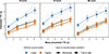 |
Figure 3. Mean estimated TTC as a function of the mean presented TTC. The different colors represent the two vehicle sound powers, with the higher sound power (audio gain 10 dB) presented in orange and the lower (audio gain 0 dB) in blue. The symbols and line types indicate the type of sound power variation, with circles and dotted lines corresponding to the trial-to-trial variation and squares and solid lines corresponding to the blockwise variation. The panels correspond to the three different velocities. Error bars show ±1 standard error of the mean across the 22 participants. |
3.2 In-depth analysis for the condition with blockwise power variation
In the rmANOVA, there was a significant interaction between the vehicle sound power (varied within subjects) and the sound power presented in the first block of the experiment (varied between subjects). To further analyze this effect, we conducted an additional rmANOVA using only the data from the first session (blockwise power variation) (see Tab. 2).
The left panel of Figure 4 shows that when participants started with the lower sound power, there was virtually no difference between the mean TTCs estimated in the higher vs. lower power conditions (mean difference M = −0.025 s, SD = 0.361 s). However, there was a large difference when participants started with the higher sound power (mean difference M = 0.596 s, SD = 0.393 s). The individual data are shown in the right panel of Figure 4. This shows that the “lack of difference” between the higher and lower sound power for participants who started with the lower sound power was consistent across participants. Only two participants showed a notable change in the estimated TTC, and the direction of this effect differed between them. On the other hand, for participants who started with the higher sound power (shown in red), the mean estimated TTC consistently increased in the second block. Post-hoc paired-samples t-tests confirmed that the effect of vehicle sound power was not significant in the group that started with the lower sound power t(10)= − 0.23, p = 0.825, but was significant in the group that started with the higher sound power t(10)=5.03, p = 0.001, dz = 1.52.
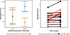 |
Figure 4. This figure only shows only data from the first session, in which the vehicle sound power was varied in a blockwise fashion. The left panel shows the mean estimated TTC as a function of the vehicle sound power presented in the first block that participants completed. Half of the 22 participants started with the block presenting the lower sound power (n = 11) and the other half with the higher sound power (n = 11). The colors indicate the vehicle sound power (orange = higher sound power, blue = lower sound power). Error bars show ±1 standard error of the mean (SEM). The right panel shows, for each participant, how the mean estimated TTC changed between their first and second block. The colors here indicate the sound power in the first block that participants completed (black = lower sound power presented in block 1, red = higher sound power presented in block 1). |
A potential reason for this difference in the effect of vehicle sound power is that the group that started with the higher sound power simply had more room to adjust their estimates in the second block. The mean estimated TTC in the first block did not differ strongly between the two groups, and the estimated TTCs were relatively short in general (extremely short in some particular cases even; see right panel in Fig. 4). As such, a shortening of the estimated TTCs in block 2 relative to block 1 would have been more restricted because the lowest possible TTC value is 0 s, compared to a lengthening of the estimated TTCs (theoretically without limit). However, the individual data for the group receiving the lower sound power in block 1 show that even participants who on average exhibited relatively long TTC judgments and would thus have had more “leeway” to shorten their estimated TTC in block 2, did not show an effect of power.
3.3 Effect of direction of TTC-change in the condition with trial-to-trial sound power variation?
Did an effect similar to the observed effect of the direction of the change in sound power from block 1 to block 2 in session 1 also occur in the trial-to-trial power variation? To answer this question, we analyzed the change in estimated TTC between the previous and current trial (i.e., trial n − 1 to trial n), as a function of the change in the final sound intensity at the participant’s position from the previous and current trial (trial n − 1 to trial n), across all pairs of consecutive trials presented in session 2 (i.e., with trial-to-trial variation in vehicle sound power). To calculate the between-trials change in final sound intensity, we analyzed the A-weighted energy equivalent sound pressure level in the last 0.5 s before occlusion (LAeqOcc) at the participant’s position, which depends not only on the presented vehicle sound power condition (i.e., audio gain of 0 or 10 dB), but also on the distance at occlusion and the vehicle speed. If, in the session with trial-to-trial sound power variation, there was an effect of the direction of the between-trials change in sound intensity, similar to the effect of the between-blocks sound power variation, then this would have resulted in an asymmetric relation between the change in LAeqOcc and the change in estimated TTC between trials. Specifically, a decrease in LAeqOcc from the previous to the current trial should have resulted in a stronger change in estimated TTC between the two trials, compared to an increase in LAeqOcc from the previous to the current trial. To evaluate this, we fitted three regression lines which relate the change in LAeqOcc from trial n − 1 to trial n to the change in estimated TTC. These fitted lines are shown in Figure 5, together with the individual datapoints for each trial. The solid gray line (diagonal line beneath the black lines) was fitted based on all trials in the trial-to-trial level variation session. The black lines were fitted depending on the direction of the change in LAeqOcc. The solid black line was fitted to trials where LAeqOcc decreased from trial n − 1 to trial n and the dashed black line was fitted to trials where LAeqOcc increased from the previous to the current trial. As visible in Figure 5, both regression lines that were fitted based on a subset of the data (black solid and dashed) overlapped almost perfectly with the regression line that was fitted on all datapoints (gray), and the relationship was symmetric with respect to the origin. In short, the data from the condition with trial-to-trial power variation do not show an effect of the direction of intensity change comparable to the data from the blockwise power variation (session 1) shown in Figure 4.
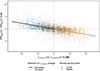 |
Figure 5. The change in estimated TTC as a function of the change in LAeqOcc on a given trial n, relative to the TTC and LAeqOcc presented on the preceding trial n − 1, in the blocks with trial-to-trial variation in sound power. The changes were calculated between pairs of consecutive trials. The colors of the individual datapoints show the vehicle sound power of trial n. The solid black regression line was fitted based on data from pairs of trials with a decrease in LAeqOcc (LAeqOcc(n)< LAeqOcc(n − 1)). The dashed black regression line was fitted based on data from pairs of trials with an increase in LAeqOcc(LAeqOcc(n)≥LAeqOcc(n − 1)). Lastly, the gray regression line was fitted to all trials from the condition with trial-to-trial sound power variation. |
3.4 Block 1 – Estimated TTCs at the lower vs. higher vehicle sound power
In the very first block of the experiment, did the difference in the “absolute” (rather than relative) power cause a difference in the estimated TTCs between the group that received the lower or higher, respectively, sound power? In the left panel of Figure 4, the mean estimated TTCs in block 1 are represented by the left blue data point (lower sound power) and the right orange data point (higher sound power). In the right panel, this corresponds to black data points on the left and red data points on the right. The average data in the left panel show a small difference in the expected direction. Participants receiving the lower sound power in block 1 estimated slightly longer TTCs (M = 1.935 s, SD = 0.863 s) than those receiving the higher sound power (M = 1.728 s, SD = 0.526 s). However, taking into account the individual data shown in the right panel, this difference was mostly due to a single participant in the lower sound power group estimating relatively long TTCs. In fact, in an additional rmANOVA analyzing only the estimated TTCs from block 1, the difference between groups (i.e., vehicle sound powers) was non-significant, F(1, 20)=0.460, p = 0.505. Note that the statistical power of this test was of course rather small because it compared two groups with only 11 participants each. A sensitivity analysis showed that with 11 participants per group, an effect size of Cohen’s d = 1.23 would have been required to be detected with a power of 1 − β = 0.8 and at an α-level of 0.05 in a two-tailed t-test for independent samples.
3.5 Summary of the effect of the type of vehicle sound power variation
To summarize the effects of sound power, in the very first block of the experiment, (session 1, block 1), we found no significant difference in the estimated TTCs between participants who heard the higher sound power vehicle (power amplified by 10 dB) and participants who heard the lower sound power vehicle (non-amplified vehicle recordings). In the next block, participants who experienced a decrease in sound power relative to block 1 increased their estimated TTCs as expected. However, participants who experienced an increase in sound power did not significantly decrease their TTC estimations. On average, there was a relatively small, but significant effect of vehicle sound power when it varied from block to block (mean difference of 0.29 s ± 0.49 s, dz = 0.59). In the second session, where the vehicle sound power varied from trial to trial, all participants showed an effect of sound power in the expected direction, and the difference in estimated TTC between the two vehicle sound powers (mean difference of 1.17 s ± 0.62 s, dz = 1.90) was considerably larger compared to the difference when the power was varied between blocks. This is compatible with the assumption that the effect of vehicle sound power is amplified by experiencing a contrast between “loud” and “soft” vehicles on a short time scale of only a few seconds (trial-to-trial sound power variation; session 2) versus a longer timescale of several minutes (blockwise power variation; session 1), and is virtually absent when participants can only rely on previous experience/familiarity with the sound power of real vehicles (between-subjects effect of vehicle sound power in block 1).
3.6 Additional effects
The rmANOVA on the full dataset (Tab. 1) showed some additional significant interaction effects, all including the sound power or type of power variation. The effect size for these effects was smaller than for the effects discussed so far, however. The effect showing the largest effect size among these additional significant effects was a TTC × sound power interaction. As shown in Figure 3, the difference between the estimated TTC at the lower and the higher sound power increased with the TTC, particularly so for the trial-to-trial power variation (and in fact, the TTC × vehicle sound power (audio gain) × type of sound power variation interaction was also significant). One potential explanation for this smaller difference at shorter TTCs could be that participants had less space to shorten their estimated TTCs, because the lower bound of TTC is 0 s.
In addition to the mean estimated TTCs, we analyzed the intra-individual variability of the estimated TTCs in each of the experimental conditions, by computing the standard deviation of the estimated TTC across the 10 trials presented to each participant per experimental condition (TTC × velocity × vehicle sound power × type of power variation; corresponding to the 48 datapoints in Fig. 3). These intra-individual standard deviations are a measure of the precision of the TTC estimates and are sometimes referred to as the “variable error”, using the terminology dating back to Fechner [53]. Figure A.2 in the appendix shows the mean of the intra-individual SDs per experimental condition, as a function of the mean estimated TTC in the same conditions. The mean intra-individual SDs ranged from 0.32 s to 1.18 s. Compatible with the literature on visual (e.g., [48, 49]), auditory (e.g., [1]), and audiovisual TTC estimation [1, 5], the mean intra-individual SDs (i.e., the mean “variable error”) increased approximately linearly with the mean estimated TTC. In fact, the observed increase of the intra-individual SD of estimated TTC by 0.19 s per increase in the mean estimated TTC by 1.0 s shown by the regression line in Figure A.2 is only slightly higher than the slope of 0.16 s/s of the linear function relating the intra-individual SD to the mean of estimated TTC in a visual-only experiment presenting a traffic scenario similar to the scenario studied here [54].
4 Discussion
This experiment investigated how the type of vehicle sound power variation (from trial to trial versus between experimental blocks) affects the size of the intensity-arrival effect in auditory TTC estimation (i.e., shorter estimated TTCs for louder compared to quieter sound sources). In line with our expectations, the results showed a shorter mean estimated TTC when the presented vehicle sound power was higher (and thus also the vehicle sound intensity at the participant’s position and the loudness of the vehicle sound was higher), compared to when the sound power was lower. The size of this effect depended on the type of sound power variation. As expected, when the sound power variation was presented in a blockwise manner, the difference in mean estimated TTC between the higher and lower sound power conditions was significant, albeit relatively small. When the level variations occurred more rapidly (i.e., from trial to trial), the differences between the two vehicle sound power conditions were much larger, in line with our reasoning that trial-to-trial changes in vehicle sound power might draw participants’ attention towards these changes.
The stimuli that were used in the present experiment were based on Oberfeld et al. [4], where they compared TTC estimations for internal combustion engine vehicles (ICEVs) and loudness-matched electric vehicles (EVs) presented at either the original vehicle sound power of the recorded ICEV (matching the lower sound power in the present paper) and with the sound power increased by 10 dB (matching the higher sound power in the present study). In Oberfeld et al. [4], the sound power varied from trial to trial. The same vehicle source signals (recordings of an ICEV) as in Oberfeld et al. [4] were used in the present experiment, so it is interesting to compare the results of the two experiments. Oberfeld et al. [4] found that on average participants estimated 0.74 s longer TTCs (dz = 2.07) for the lower vehicle sound power in an auditory-only condition with trial-to-trial sound power variation, averaged across vehicle type and velocity. In comparison, in the presented experiment, participants on average estimated 1.17 s longer TTCs (dz = 1.90) at the lower sound power in the same condition (auditory-only, trial-to-trial power variation), averaged across velocity. Both experiments thus show a similarly large effect of vehicle sound power on the mean estimated TTC (intensity-arrival effect).
4.1 Results are not compatible with a reliance on familiar vehicle sound power
The fixed presentation order of the two types of vehicle sound power variation allowed us to compare the TTC estimations between two groups of participants that either received only the lower or only the higher sound power in the very first block of the experiment. In this block, the “absolute” sound power differed between groups, but participants neither experienced a change in sound power within the block, nor had any within-experiment comparison with a different vehicle sound power. The data (Fig. 4) indicated no significant difference in the mean estimated TTCs between these two groups (i.e., the two vehicle sound powers) in the first block. Thus, the difference in the “absolute” (rather than relative) sound power did not result in systematically different estimated TTCs. This would suggest that participants may not have access to a representation of “familiar vehicle sound power”, i.e., a prior expectation of vehicle sound power. The deviation from such a familiar sound power in the two sound power conditions should have resulted in a significant difference in mean estimated TTC between the two groups receiving either the higher or the lower sound power in block 1. In the visual domain, Hosking and Crassini [26] found that the size-arrival effect was reduced when the objects were of a known size (football vs. tennis ball; shown to the participants before the experiment) compared to non-textured spheres of the same sizes. In contrast when the objects were presented with an incongruent size (football at tennis ball size and vice versa), the size-arrival effect was enhanced, suggesting that participants relied to some extent upon the known size of the objects. The visual size of an object and the perceived sound intensity at the receiver position are both “heuristic” (i.e., not perfectly reliable) cues to the distance of the object, unless the sound power and object size are known exactly. If the sound power or object size was known (“familiar”) through prior experience, then the sound power/optical size at occlusion would be no longer merely a heuristic, but an accurate distance cue, at least for sources that do not deviate strongly from the learned sound power. For sources that do deviate from the familiar sound power, however, misestimations of the distance and thus the TTC would result. That is, if participants used a memory reference for vehicle sound power based on previous experience with vehicles, we would expect a difference between the group receiving the higher and the group receiving the lower sound power in the very first block. The absence of such an effect might suggest that participants build up an internal reference of vehicle sound power only within the experiment (i.e., from block to block), instead of relying on a “familiar sound level” established before the experiment. However, the between-subjects comparison between the mean estimated TTCs for the very first block of the present experiment must be viewed with some caution due to the small sample size.
4.2 Central-tendency effect in auditory TTC estimation
Apart from the effect of sound power, the present experiment showed a “central tendency” [47] response pattern where the range of estimated TTCs is smaller than the range of presented TTCs. Such a pattern was consistently observed in previous studies on auditory-only TTC estimation (e.g., [1, 4]), but also in visual-only TTC estimation (e.g., [48–50]). Central-tendency effects are often assumed to suggest a reliance on prior information, in the spirit of Bayesian observer models (see, e.g., [55]), which might be amplified by a factual or perceived unreliability of the auditory cues. We believe that further improvements of the acoustic simulations might result in a slight reduction of this effect. In fact, compared to the A-only condition in Oberfeld et al. [4] that presented very similar stimuli, the central-tendency pattern was less pronounced in the present study. This might be the result of an improvement in the acoustic setup between experiments. The 16-loudspeaker array used in Oberfeld et al. [4] was expanded to a 41-loudspeaker array for the present experiment, enabling rendering of the spatial sound fields with a higher spatial resolution. Therefore, a reduction in the central-tendency pattern might in part be the result of an improved reliability of auditory cues. Another relevant aspect is that sound-intensity cues to the TTC of approaching vehicles [1, 56, 57] show a certain inherent unreliability, because – unlike for laboratory sounds such as sine waves or broadband noise – the sound power of vehicles with combustion engine is not stationary but shows some motion-unrelated fluctuations across time. These sound power fluctuations, resulting in fluctuations of the vehicle sound intensity at the pedestrian’s position, represent “external noise” [58] that reduces the precision of intensity-based TTC cues. A combination between this inherent unreliability and limitations in the perceptual processing of the relevant acoustic cues might be the origin of the central tendency response pattern, but additional research is needed to understand these effects. Some previous papers also showed a tendency towards an underestimation of the TTC in an auditory-only condition, both compared to the veridical TTC value and the mean estimated TTCs in conditions with additional visual information [1, 4, 5, 51]. At present, it is unclear whether this can be interpreted as a “safety strategy” (better underestimate than overestimate the TTC when a precise estimation is difficult), or can be linked to characteristics of the auditory TTC cues.
4.3 Limitations
Several questions remain open due to limitations of our study and should be addressed in future research. Firstly, as explained before, there was an error in the computation of the sound propagation that resulted in a deviation in the presented TTC, which depended both on the intended TTC and the velocity. As such, results regarding the effects of velocity and presented TTC on the estimated TTCs should be interpreted with care. However, the focus of our study was on the effect of vehicle sound power and how this depends on the type of sound power variation. Since the technical issue affected both the lower and higher sound power conditions equally, we consider our central results unaffected by this programming error.
Secondly, we, intentionally, did not counterbalance the presentation order of the type of vehicle sound power variation. Our motivation for this, as also explained above, was that our study focused on the effects of blockwise power variation. We did not want participants to have a within-experiment level reference in the first block of the blockwise power variation, so that we could properly test if an effect of vehicle sound power (the intensity-arrival effect) would also occur between subjects in this block. It would be interesting to additionally include groups that start with a trial-to-variation variation in vehicle sound power. This group would be presented with the full range of vehicle sound powers already in the first block and, thus, can make within-experiment vehicle sound power comparisons in the following blocks with blockwise power variation. We would expect that participants in this group would transfer their longer TTC estimations for vehicles with lower and shorter TTC estimations for vehicles with higher sound power to the session with blockwise power variation, resulting in a stronger effect of the blockwise power variation than in the present design.
Lastly, while we aimed for the virtual environments and stimuli to be as accurate as possible, there are of course limitations to both the auditory vehicle simulation and the verisimilitude of the visual scene. Most important, we did not present the approaching vehicles visually in the present experiment. In real-life traffic scenarios, in contrast, pedestrians typically both see and hear the approaching vehicle, unless a pedestrian is listening to loud music over headphones that masks the vehicle sound [59], the sound of the approaching vehicle is masked by loud ambient noise such as traffic from a neighboring highway, or a pedestrian is visually impaired or cannot use vision for other reasons. Based on previous results [4, 5], we would expect the effect of vehicle sound power on TTC estimation to be reduced when visual information about the vehicle’s motion is available, although we would again expect a stronger effect of trial-to-trial compared to blockwise sound power variation.
4.4 Implications of the effects of vehicle sound power on TTC estimation for traffic safety
In everyday traffic scenarios, the sound power of vehicles approaching a pedestrian can vary on a relatively long time scale, as in the condition with blockwise power variation in the present experiment, or on a shorter time scale, as in the experimental condition with trial-to-trial power variation. For the blockwise power variation, imagine for example two roads with two different surfaces, e.g., cobblestones versus a modern low-noise asphalt surface. The same set of vehicles (driving the same speed on the both roads) would produce a considerably higher sound level at the position of pedestrians at the roadside (i.e., sound louder) on the cobblestone road compared to the low-noise asphalt road, due to the differences in tire-road noise between the two surface types, e.g., [8, 9]. Thus, the situation is equivalent to our experimental condition with blockwise sound power variation where there was an overall shift in the vehicle sound levels encountered by participants between blocks. The results of the present experiment suggest that the difference in vehicle sound power between the two road types should have only a relatively small effect on pedestrians’ TTC judgments. This appears plausible because one should expect the pedestrian to take into account that on a given road, all approaching vehicles might sound either somewhat louder or somewhat quieter.
In contrast, on a given road surface, regardless of the average sound power of the vehicles driving on that road, different vehicle types or different tire types [9] will result in sound power differences between consecutive vehicles, even if all vehicles are approaching at the same speed. For instance, a relatively quiet small passenger car with electric engine and narrow tires might be followed directly by a considerably louder large heavy-duty vehicle with diesel engine and wide tires. Based on the results from the condition with trial-to-trial sound power variation of the present experiment, we would expect that the difference in sound power between vehicles will have a significant effect on the pedestrian’s TTC judgments, because the resulting variation of the vehicle sound intensity at the pedestrians’ position occurs on a relatively short time scale.
This effect of vehicle sound power on the estimated TTC can be expected to affect street-crossing decisions. To make a safe crossing decision, the optimal strategy would be to compare the arrival time of a vehicle with the time it would take them to cross the road. Only if the time remaining before the vehicle will arrive at the pedestrian’s position is longer than the time it would take them to cross the road, plus some safety margin, then a pedestrian can cross safely. Biases in TTC estimation effected by changes in vehicle sound power should thus influence street-crossing decisions. If pedestrians perceive a quieter car to take longer to arrive at their position than a louder car with the same actual TTC, they might accept shorter TTCs (i.e., shorter time gaps) for the quieter car, resulting in an increased risk of collision. This could be particularly concerning in the context of electric vehicles, which are, at low velocities, on average quieter than internal combustion engine vehicles. A recent study from our lab [60] provided evidence for this hypothesis. The data showed an effect of vehicle sound power, which varied from trial to trial, on street-crossing decisions. Participants made riskier crossing decisions for vehicles presented with a lower sound power, compatible with the overestimated TTCs at the lower sound power observed in the present study and in previous experiments [4, 17]. This suggests an increased risk of pedestrians being hit by quieter vehicles. Indeed, incidence rates [20–22] show higher odds of collisions between pedestrians or bicyclists and electric vehicles, compared to internal combustion engine vehicles.
Because the results of the present study show that the effect of vehicle sound power on TTC estimation depends on the time scale in which the sound power variations occur, the riskiness of crossing decisions in interaction with quieter vehicles might be, in part, due to these vehicles occurring alongside louder vehicles. Additional experiments should explore this further, which will be relevant to predict whether quieter vehicles pose less risk to pedestrians when no louder vehicles are present in a street-crossing scenario.
Acknowledgments
We are grateful to Tim Niewalda, Jan Schmitz and Simon Benedikt Schaefer for collecting the data.
Funding
This work was supported by funding from Deutsche Forschungsgemeinschaft granted to Daniel Oberfeld (grant number OB 346/8-1; priority program AUDICTIVE – SPP2236: Auditory Cognition in Interactive Virtual Environments). The funders had no role in study design, in the collection, analysis and interpretation of the data, in the writing of the report, and in the decision to submit the article for publication.
Conflict of interest
The authors declare no conflict of interest.
Data availability statement
The primary data are available in OSF.io, under the reference [61].
Author contribution statement
Thirsa Huisman: Conceptualization (equal), Data curation, Formal Analysis (equal), Investigation, Methodology (supporting), Resources (equal), Software (lead), Visualization (lead), Writing – original draft (equal), Writing – review & editing. Daniel Oberfeld: Conceptualization (equal), Formal Analysis (equal), Funding acquisition, Methodology (lead), Project administration, Resources (equal), Software (supporting), Supervision, Visualization (supporting), Writing – original draft (equal), Writing – review & editing. Patricia DeLucia: Writing – review & editing.
References
- P.R. DeLucia, D. Preddy, D. Oberfeld: Audiovisual integration of time-to-contact information for approaching objects. Multisensory Research 29, 4–5 (2016) 365–395. [Google Scholar]
- P.R. DeLucia: Pictorial and motion-based information for depth perception. Journal of Experimental Psychology: Human Perception and Performance 17, 3 (1991) 738–748. [Google Scholar]
- B. Keshavarz, J.L. Campos, P.R. DeLucia, D. Oberfeld: Estimating the relative weights of visual and auditory tau versus heuristic-based cues for time-to-contact judgments in realistic, familiar scenes by older and younger adults. Attention, Perception, & Psychophysics 79, 3 (2017) 929–944. [Google Scholar]
- D. Oberfeld, M. Wessels, D. Büttner: Overestimated time-to-collision for quiet vehicles: evidence from a study using a novel audiovisual virtual-reality system for traffic scenarios. Accident Analysis & Prevention 175 (2022) 106778. [Google Scholar]
- P.R. DeLucia, D. Oberfeld, J.K. Kearney, M. Cloutier, A.M. Jilla, A. Zhou, et al.: Visual, auditory, and audiovisual time-to-collision estimation among participants with age-related macular degeneration compared to a normal-vision group: the TTC-AMD study. PLoS One 20, 12 (2025) e0337549. [Google Scholar]
- P. Zeller, Ed.: Handbuch Fahrzeugakustik [Vehicle Acoustics Handbook]. Springer, Berlin, 2018. [Google Scholar]
- W.M. Hartmann: Signals, Sound, and Sensation, 5th edn. Springer, New York, 2005. [Google Scholar]
- U. Sandberg: Road traffic noise - The influence of the road surface and its characterization. Applied Acoustics 21, 2 (1987) 97–118. [Google Scholar]
- U. Sandberg, Ed.: Tyre/road noise - Myths and realities, in: Internoise, International Congress and Exhibition on Noise Control Engineering, 2001, Nederlands Akoestisch Genootschap, Maastricht, 2001b. [Google Scholar]
- European Commission: Commission Directive (EU) 2015/996 of 19 May 2015 establishing common noise assessment methods according to Directive 2002/49/EC of the European Parliament and of the Council (CNOSSOS-EU), 2015. [Google Scholar]
- S. Kephalopoulos, M. Paviotti, F. Anfosso-Lédée: Common Noise Assessment Methods in Europe (CNOSSOS-EU). JCR Reference Report EUR 25379 EN. Luxembourg: European Commission Joint Research Centre. Institute for Health and Consumer Protection, 2012. Available from: https://publications.jrc.ec.europa.eu/repository/handle/JRC72550. [Google Scholar]
- L. Garay-Vega, A. Hastings, J.K. Pollard, M. Zuschlag, M.D. Stearns: Quieter Cars and the Safety of Blind Pedestrians: Phase 1. U.S. Department of Transportation, National Highway Traffic Safety Administration, 2010. Available from: https://rosap.ntl.bts.gov/view/dot/9474/dot_9474_DS1.pdf. [Google Scholar]
- M.-A. Pallas, J. Kennedy, I. Walker, R. Chatagnon, M. Berengier, J. Lelong: Noise emission of electric and hybrid electric vehicles: deliverable FOREVER (n° Forever WP2_D2-1-V4). Institut Français des Sciences et Technologies des Transports, del’Aménagement et des Réseaux, 2015. [Google Scholar]
- M. Pilgersdorfer, K. Runda, M. Conter, M. Gatscha, A. Pumberger, A.M. Müller, et al.: drivEkustik - Fahrverhalten in und akustische Wahrnehmung von Elektrofahrzeugen. Wien Bundesministerium für Verkehr, Innovation und Technologie, 2013. [Google Scholar]
- W. Jesteadt, L. Leibold: Loudness in the laboratory, Part I: steady-state sounds, in: M. Florentine, A.N. Popper, R.R. Fay, Eds. Loudness. Springer, 2011, pp. 109–144. [Google Scholar]
- M.S. Horswill, S. Helman, P. Ardiles, J.P. Wann: Motorcycle accident risk could be inflated by a time to arrival illusion. Optometry and Vision Science 82, 8 (2005) 740–746. [Google Scholar]
- P.R. DeLucia: Effects of size on collision perception and implications for perceptual theory and transportation safety. Current Directions in Psychological Science 22, 3 (2013) 199–204. [Google Scholar]
- C.W. Pai: Motorcycle right-of-way accidents-A literature review. Accident Analysis & Prevention 43, 3 (2011) 971–982. [Google Scholar]
- C. Mundutéguy, I. Ragot-Court: A contribution to situation awareness analysis: understanding how mismatched expectations affect road safety. Human Factors 53, 6 (2011) 687–702. [Google Scholar]
- R. Hanna: Incidence of pedestrian and bicyclist crashes by hybrid electric passenger vehicles. National Highway Traffic Safety Administration 2009 DOT HS 811 204, Washington, DC, 2009. [Google Scholar]
- E. Verheijen, J. Jabben: Effect of electric cars on traffic noise and safety. National Institute of Public Health and Environmental Protection RIVM, Netherlands, 2010. [Google Scholar]
- J. Wu, R. Austin, C.-L. Chen: Incidence rates of pedestrian and bicyclist crashes by hybrid electric passenger vehicles: an update (DOT HS 811 526). National Highway Traffic Safety Administration, Washington, DC, 2011. [Google Scholar]
- J.K. Caird, P.A. Hancock: The perception of arrival time for different oncoming vehicles at an intersection. Ecological Psychology 6, 2 (1994) 83–109. [Google Scholar]
- B. Sidaway, M. Fairweather, H. Sekiya, J. McNittGray: Time-to-collision estimation in a simulated driving task. Human Factors 38, 1 (1996) 101–113. [Google Scholar]
- P.R. DeLucia: Does binocular disparity or familiar size information override effects of relative size on judgements of time to contact? Quarterly Journal of Experimental Psychology Section A: Human Experimental Psychology 58, 5 (2005) 865–886. [Google Scholar]
- S.G. Hosking, B. Crassini: The effects of familiar size and object trajectories on time-to-contact judgements. Experimental Brain Research 203, 3 (2010) 541–552. [Google Scholar]
- G. Grimm, J. Luberadzka, V. Hohmann: A toolbox for rendering virtual acoustic environments in the context of audiology. Acta Acustica United with Acustica 105, 3 (2019) 566–578. [CrossRef] [Google Scholar]
- ISO 9613-2:1999-10: Acoustics - Attenuation of sound during propagation outdoors - Part 2: general method of calculation, 1999. [Google Scholar]
- G. Grimm, V. Hohmann: First order Ambisonics field recordings for use in virtual acoustic environments in the context of audiology, 2019. Available from: https://zenodo.org/record/3588303. [Google Scholar]
- J.B. Allen, D.A. Berkley: Image method for efficiently simulating small-room acoustics. Journal of the Acoustical Society of America 65, 4 (1979) 943–950. [Google Scholar]
- J. Ahrens, R. Rabenstein, S. Spors: Sound field synthesis for audio presentation. Acoustics Today 10, 2 (2014) 15–25. [Google Scholar]
- M.A. Gerzon: Ambisonics in multichannel broadcasting and video. Journal of the Audio Engineering Society 33, 11 (1985) 859–871. [Google Scholar]
- J. Daniel: Représentation de champs acoustiques, application é la transmission et é la reproduction de scènes sonores complexes dans un contexte multimédia: Université Pierre et Marie Curie (Paris VI), 2000. [Google Scholar]
- V. Pulkki: Virtual sound source positioning using vector base amplitude panning. Journal of the Audio Engineering Society 45, 6 (1997) 456–466. [Google Scholar]
- W. Schiff, M.L. Detwiler: Information used in judging impending collision. Perception 8, 6 (1979) 647–658. [Google Scholar]
- W.L. Carel: Visual factors in the contact analog (Publication R61ELC60). General Electric Company Advanced Electronics Center, Ithaca, NY, 1961. [Google Scholar]
- D.A. Rosenbaum: Perception and extrapolation of velocity and acceleration. Journal of Experimental Psychology: Human Perception and Performance 1, 4 (1975) 395–403. [Google Scholar]
- UNECE R138: Regulation No 138 of the Economic Commission for Europe of the United Nations (UNECE) - Uniform provisions concerning the approval of Quiet Road Transport Vehicles with regard to their reduced audibility, 2017. [Google Scholar]
- H. Steven: Investigations on noise emission of motor vehicles in road traffic: Umweltbundesamt, 2005, https://www.umweltbundesamt.de/sites/default/files/medien/publikation/long/3092.pdf. [Google Scholar]
- P.L. Smith, D.R. Little: Small is beautiful: in defense of the small-N design. Psychonomic Bulletin & Review 25, 6 (2018) 2083–2101. [CrossRef] [PubMed] [Google Scholar]
- M. Brysbaert, M. Stevens: Power analysis and effect size in mixed effects models: a tutorial. Journal of Cognition 1, 1 (2018) 9. [CrossRef] [PubMed] [Google Scholar]
- J. Cohen: Statistical Power Analysis for the Behavioral Sciences, 2nd edn. L. Erlbaum Associates, Hillsdale, N.J., 1988. [Google Scholar]
- G. Békésy: A new audiometer. Acta Oto-Laryngologica (Stockholm) 35, 5–6 (1947) 411–422. [Google Scholar]
- A.G. Bennett, R.B. Rabbetts: Clinical Visual Optics, 3rd edn. Vol. viii. Butterworth-Heinemann, Oxford, Boston, 1998, 451 pp. [Google Scholar]
- J.W. Tukey: Exploratory Data Analysis. Addison-Wesley Pub. Co., Reading, Mass., 1977. [Google Scholar]
- H. Huynh, L.S. Feldt: Estimation of the Box correction for degrees of freedom from sample data in randomized block and split-plot designs. Journal of Educational Statistics 1, 1 (1976) 69–82. [CrossRef] [Google Scholar]
- H.L. Hollingworth: The central tendency of judgment. Journal of Philosophy, Psychology & Scientific Methods 7 (1910) 461–469. [Google Scholar]
- D. Oberfeld, H. Hecht: Effects of a moving distractor object on time-to-contact judgments. Journal of Experimental Psychology: Human Perception and Performance 34, 3 (2008) 605–623. [Google Scholar]
- H. Heuer: Estimates of time to contact based on changing size and changing target vergence. Perception 22, 5 (1993) 549–563. [Google Scholar]
- R.W. McLeod, H.E. Ross: Optic flow and cognitive factors in time-to-collision estimates. Perception 12, 4 (1983) 417–423. [Google Scholar]
- W. Schiff, R. Oldak: Accuracy of judging time to arrival: effects of modality, trajectory, and gender. Journal of Experimental Psychology: Human Perception and Performance 16, 2 (1990) 303–316. [Google Scholar]
- Y. Hochberg: A sharper Bonferroni procedure for multiple tests of significance. Biometrika 75, 4 (1988) 800–802. [Google Scholar]
- G.T. Fechner: Elemente der Psychophysik. Vol. 2. Breitkopf und Härtel, Leipzig, 1860, 1 p. [Google Scholar]
- M. Wessels, D. Oberfeld: A binary acceleration signal reduces overestimation in pedestrians’ visual time-to-collision estimation for accelerating vehicles. Heliyon 10, 6 (2024) e27483. [Google Scholar]
- Z.H. Shi, R.M. Church, W.H. Meck: Bayesian optimization of time perception. Trends in Cognitive Sciences 17, 11 (2013) 556–564. [Google Scholar]
- B.K. Shaw, R.S. McGowan, M.T. Turvey: An acoustic variable specifying time-to-contact. Ecological Psychology 3, 3 (1991) 253–261. [Google Scholar]
- R.L. Jenison: On acoustic information for motion. Ecological Psychology 9, 2 (1997) 131–151. [Google Scholar]
- J.A. Swets, E.F. Shipley, M.J. McKey, D.M. Green: Multiple observations of signals in noise. Journal of the Acoustical Society of America 31, 4 (1959) 514–521. [CrossRef] [Google Scholar]
- R. Lichenstein, D.C. Smith, J.L. Ambrose, L.A. Moody: Headphone use and pedestrian injury and death in the United States: 2004–2011. Injury Prevention 18, 5 (2012) 287–290. [Google Scholar]
- D. Oberfeld, T. Huisman, P.R. DeLucia: Quieter vehicles result in riskier pedestrian street-crossing decisions. Preprint 2026. DOI: https://doi.org/10.31234/osf.io/nykfm_v2. [Google Scholar]
- D. Oberfeld, T. Huisman: Dataset: the effect of vehicle sound intensity on auditory-only time-to-collision estimation, 2025. DOI: https://doi.org/10.17605/OSF.IO/7DQGJ. [Google Scholar]
Appendix A
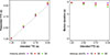 |
Figure A.1. Left panel: Scatter plot of the presented TTC at occlusion as a function of the intended TTC, across all trials presented in the experiment. The presented TTC was always slightly longer than the intended TTC (indicated by the diagonal). Purple: vehicle speed 10 km/h. Red: 30 km/h. Green: 50 km/h. Right panel: Scatterplot of the presented motion duration as a function of intended TTC. The intended duration of 3 s is indicated by the gray horizontal line. |
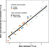 |
Figure A.2. Mean of the intra-individual standard deviation of the estimated TTCs, plotted as a function of the mean estimated TTC. Each data point corresponds to one of the experimental conditions (i.e., unique combinations of TTC, velocity, vehicle sound power, and type of power variation; same as the data points plotted in Fig. 3). Orange symbols: higher sound power. Blue symbols: lower sound power. Filled squares: blockwise source-power variation. Open circles: trial-to-trial power variation. The black line shows the best-fitting linear regression line, SD(TTCest)=0.22 s + 0.19 M(TTCest), R2 = 0.89. |
Cite this article as: Huisman T. DeLucia P.R. & Oberfeld D. 2026. The effect of vehicle sound power on auditory time-to-collision estimation. Acta Acustica, 10, 23. https://doi.org/10.1051/aacus/2026019.
All Tables
Results of the rmANOVA conducted on the complete dataset. Pvehicle: vehicle sound power (lower or higher, i.e., audio gain of 0 or 10 dB). ToPV: type of sound power variation. v: velocity. Pvehicle block 1: sound power presented in the first block. Displayed are F-values, numerator and denominator degrees of freedom, p-values, and the Huynh–Feldt correction factor . As measures of effect size, we report partial η2 (, dz [42] in the case of within-subjects effects with one numerator degree of freedom, and d [42] for the between-subjects effect. Bold font indicates significant effects (p < 0.05).
All Figures
|
Figure 1. The top-left panel shows one of the authors wearing the head-mounted display in the loudspeaker array. The upper ring contains 32 loudspeakers positioned at approximately ear height. The lower ring contains 8 loudspeakers angled up towards the participant. The subwoofer is not visible in the picture. The bottom-left panel shows a screenshot of the visual scene. Note that the approaching vehicle was not presented visually. The right panel shows a bird’s eye view of the simulated scene (to scale). The positions of sources and receiver are indicated in dark gray. The coordinates labelled LF, hood, RF, and RR represent the position of the four vehicle sound sources relative to the center of the front of the car, which played back the sound from the microphones positioned at the left front tire, hood, right front tire, and right rear tire, respectively. |
| In the text | |
|
Figure 2. Graphical illustration of blocks presented in each session. Bars represent individual trials, and the bar height represents the actual vehicle sound power (including the comparably small variability between trials in the same vehicle sound power condition due to e.g., differing speeds). The orange and blue bars indicate trials presenting the higher (audio gain 10 dB) and lower vehicle sound power (audio gain 0 dB), respectively. All participants started with the blockwise vehicle sound power variation. Half of the participants started with the lower sound power and the other half started with the higher sound power. In the second session, the higher and lower sound powers were presented interleaved (trial-to-trial power variation). |
| In the text | |
|
Figure 3. Mean estimated TTC as a function of the mean presented TTC. The different colors represent the two vehicle sound powers, with the higher sound power (audio gain 10 dB) presented in orange and the lower (audio gain 0 dB) in blue. The symbols and line types indicate the type of sound power variation, with circles and dotted lines corresponding to the trial-to-trial variation and squares and solid lines corresponding to the blockwise variation. The panels correspond to the three different velocities. Error bars show ±1 standard error of the mean across the 22 participants. |
| In the text | |
|
Figure 4. This figure only shows only data from the first session, in which the vehicle sound power was varied in a blockwise fashion. The left panel shows the mean estimated TTC as a function of the vehicle sound power presented in the first block that participants completed. Half of the 22 participants started with the block presenting the lower sound power (n = 11) and the other half with the higher sound power (n = 11). The colors indicate the vehicle sound power (orange = higher sound power, blue = lower sound power). Error bars show ±1 standard error of the mean (SEM). The right panel shows, for each participant, how the mean estimated TTC changed between their first and second block. The colors here indicate the sound power in the first block that participants completed (black = lower sound power presented in block 1, red = higher sound power presented in block 1). |
| In the text | |
|
Figure 5. The change in estimated TTC as a function of the change in LAeqOcc on a given trial n, relative to the TTC and LAeqOcc presented on the preceding trial n − 1, in the blocks with trial-to-trial variation in sound power. The changes were calculated between pairs of consecutive trials. The colors of the individual datapoints show the vehicle sound power of trial n. The solid black regression line was fitted based on data from pairs of trials with a decrease in LAeqOcc (LAeqOcc(n)< LAeqOcc(n − 1)). The dashed black regression line was fitted based on data from pairs of trials with an increase in LAeqOcc(LAeqOcc(n)≥LAeqOcc(n − 1)). Lastly, the gray regression line was fitted to all trials from the condition with trial-to-trial sound power variation. |
| In the text | |
|
Figure A.1. Left panel: Scatter plot of the presented TTC at occlusion as a function of the intended TTC, across all trials presented in the experiment. The presented TTC was always slightly longer than the intended TTC (indicated by the diagonal). Purple: vehicle speed 10 km/h. Red: 30 km/h. Green: 50 km/h. Right panel: Scatterplot of the presented motion duration as a function of intended TTC. The intended duration of 3 s is indicated by the gray horizontal line. |
| In the text | |
|
Figure A.2. Mean of the intra-individual standard deviation of the estimated TTCs, plotted as a function of the mean estimated TTC. Each data point corresponds to one of the experimental conditions (i.e., unique combinations of TTC, velocity, vehicle sound power, and type of power variation; same as the data points plotted in Fig. 3). Orange symbols: higher sound power. Blue symbols: lower sound power. Filled squares: blockwise source-power variation. Open circles: trial-to-trial power variation. The black line shows the best-fitting linear regression line, SD(TTCest)=0.22 s + 0.19 M(TTCest), R2 = 0.89. |
| In the text | |
Current usage metrics show cumulative count of Article Views (full-text article views including HTML views, PDF and ePub downloads, according to the available data) and Abstracts Views on Vision4Press platform.
Data correspond to usage on the plateform after 2015. The current usage metrics is available 48-96 hours after online publication and is updated daily on week days.
Initial download of the metrics may take a while.