


| Issue |
Acta Acust.
Volume 10, 2026
|
|
|---|---|---|
| Article Number | 52 | |
| Number of page(s) | 19 | |
| DOI | https://doi.org/10.1051/aacus/2026050 | |
| Published online | 30 June 2026 | |
Musical Acoustics
Quantifying the variability in Mansour nay: a stochastic approach combining vibroacoustic modelling and PCE-Kriging
1
Department of Mechanical Engineering, Alanya Alaaddin Keykubat University, Antalya 07425, Türkiye
2
Turkish Music, Istanbul Medeniyet University, Istanbul 34720, Türkiye
3
Department of Industrial Engineering, Alanya Alaaddin Keykubat University, Antalya 07425, Türkiye
* Corresponding author: This email address is being protected from spambots. You need JavaScript enabled to view it.
Received:
3
March
2026
Accepted:
19
May
2026
Abstract
The Mansour nay is a woodwind instrument made from a single piece of giant reed (Arundo donax L.). Because the body is natural and cannot be modified after construction, geometric variability across specimens is inevitable and directly affects the pitch frequencies produced by the instrument. Identifying which geometric parameters contribute most to this variability is essential for instrument makers selecting raw material and determining finger hole locations. In this study, 26 Mansour nay samples manufactured from giant reeds of different ages and geographic origins are investigated through audio-based pitch measurements, vibroacoustic finite element modelling, and uncertainty quantification. An Average Mansour Nay Model (AMNM) is constructed from the measured geometric properties of all samples and used as a reference for quantifying specimen-to-specimen deviations. Polynomial chaos expansion combined with Kriging (PCE-Kriging) is employed as a surrogate modelling technique suited to small datasets, and the expansion coefficients are used to rank the contribution of each geometric variable to the observed variability. The analysis identifies the top and bottom diameters as the dominant sources of pitch-frequency variation, with comparable influence, followed by the distances between finger holes, and then the total length. As a complementary methodological demonstration, the same PCE-Kriging framework is applied to the structural eigenfrequencies of the instrument measured under free boundary conditions, where the bottom diameter and mass emerge as the statistically significant variables. The acoustic findings provide quantitative guidance for giant reed selection and finger hole placement in nay making, and the overall methodology is transferable to other instruments made from natural materials where specimen variability is inherent.
Key words: Woodwind musical instruments / Uncertainty quantification / Polynomial chaos expansion-Kriging / Acoustic response
© The Author(s), Published by EDP Sciences, 2026
 This is an Open Access article distributed under the terms of the Creative Commons Attribution License (https://creativecommons.org/licenses/by/4.0), which permits unrestricted use, distribution, and reproduction in any medium, provided the original work is properly cited.
1. Introduction
Wind instruments are traditionally classified into two groups: woodwind instruments, played with a vibrating reed or by blowing air through an open hole, and brass instruments, played by lip vibration into a metal mouthpiece [1–3]. The nay is a woodwind instrument with an ancient history that can be considered an ancestor of the modern flute family [4]. Unlike most wind instruments that are assembled from multiple manufactured components, the nay is made from a single piece of 9-internode giant reed (Arundo donax L.) [5]. Since the body is natural and cannot be structurally modified after construction, luthiers must select candidate giant reeds based on experience, evaluating their length, wall thickness, and overall condition [6, 7]. After selection, the giant reeds are dried for approximately two years, during which moisture loss proceeds toward equilibrium moisture content and the material largely takes its final shape. Finger holes are then drilled according to a measurement system that defines a fixed tuning scheme (Fig. 1). The type known as the Mansour nay, with an average length of approximately 775 mm, is widely manufactured and used in Turkish music. Its scale spans eight notes within one octave, from G4 to G5, and corresponds to specific maqam pitches used in Turkish music theory; interested readers are referred to [8, 9] for further details.
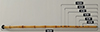 |
Figure 1. The measurement rule applied by luthiers in determining finger hole locations. |
The fundamental challenge in studying the Mansour nay, and more broadly any instrument made from natural material, is variability. Since giant reed is a natural material, no two specimens are geometrically or materially identical. Even when the total lengths are matched, the internal geometry (inner and outer diameters, wall thickness distribution along the internodes) and the mechanical properties of the material will differ from one specimen to the next. This variability propagates to the acoustic behaviour of the instrument and ultimately affects its pitch frequencies.
The physical relationship between the instrument’s material and its acoustic output requires careful framing. For a straight, narrow-bore woodwind such as the nay, the internal acoustic pressure field is essentially one-dimensional, and coupling between structural wall vibrations and the internal air column is negligible, as is well established for tube-like woodwinds such as the clarinet and flute [10]. The bore geometry, namely length, diameters, and tone hole positions, is therefore the primary determinant of pitch frequencies. The material nevertheless plays a secondary but non-negligible role, not through wall vibration, but through the properties of the internal bore surface: surface roughness, porosity, and hygroscopic behaviour during play influence the viscothermal losses that shape the damping of each acoustic resonance, and consequently the perceived timbre and playability. These material effects are not the focus of the present study; instead, we concentrate on the geometric sources of variability that can be assessed and controlled by the instrument maker at the reed-selection and finger-hole-drilling stages.
For luthiers, the practical consequence is that the process of selecting giant reeds and determining finger hole locations remains largely empirical, guided by tradition and experience rather than quantitative criteria. Identifying which physical variables are the dominant sources of variation would provide a rational basis for these decisions. Beyond instrument making, understanding the mechanical and acoustic properties of natural materials has implications for sustainability. Climate change and tightening environmental regulations are increasingly threatening the availability of wood species traditionally used in instrument manufacturing. Composite materials have already been introduced as alternatives in several instrument families [11–13], and the development of suitable replacements requires quantitative knowledge of the properties expected from the original natural material. The methodology developed in the present study contributes to this broader objective.
The role of material variability in musical instruments has been the subject of growing scientific interest. In the context of string instruments, Brauchler et al. [14] demonstrated that material variability in wood is a significant source of uncertainty in guitar making, and proposed geometry modifications predicted by finite element (FE) models to compensate for differences in material properties between guitar soundboards. The same group [15] also used possibilistic methods to identify material parameters in a parametrically reduced FE model of a classical guitar. Viala et al. [16] performed stochastic analyses on guitar soundboards with different bracing patterns, accounting for both material and climatic uncertainties, and showed that design choices dominate over material variability in the low-frequency dynamic behaviour. In a complementary study, Viala et al. [17] validated a physics-based model of a Spanish guitar soundboard against experimental data and performed screening analyses to rank the influence of material and climatic parameters on the dynamics. In a more recent model-based ranking study, Viala et al. [18] analysed the relative influence of geometry and materials on the dynamical behaviour of the violin and highlighted the predominance of geometrical choices. These studies demonstrate the value of combining computational models with stochastic methods for understanding variability in instruments made of natural materials. However, they focus exclusively on string instruments composed of multiple assembled parts (soundboard, braces, back plate), where design variables can be adjusted independently.
For wind instruments, computational modelling has primarily focused on bore geometry optimisation and acoustic characterisation. Ernoult et al. [19] used full waveform inversion to reconstruct the bore geometry of woodwind-like instruments from impedance measurements. Noreland et al. [20] optimised the tone hole geometry of a clarinet-like instrument to improve intonation. Cabaret et al. [21] developed an experimental database for the validation of resonator models, comparison of geometries and materials, and quantification of measurement errors in wind instruments. These studies address deterministic design problems, or validation of resonator models, rather than quantifying the variability across a population of instruments. To the authors’ knowledge, no study has applied uncertainty quantification (UQ) methods to a population of wind instruments made from natural material to identify which geometric variables drive the observed variation. Couineaux et al. [22] more generally developed a minimal physical model of the cristal Baschet combining FE modal analysis with friction-induced vibration models, illustrating the broader applicability of FE-based stochastic approaches to non-wind musical instruments.
The present study addresses this gap. Twenty-six Mansour nay samples are manufactured from giant reeds collected from four different geographic regions and with three different age ranges. All instruments are played by a professional performer, and their pitch frequencies are extracted from audio recordings. One sample is subsequently sacrificed for 3D scanning to obtain detailed internal geometry; consequently, all 26 samples are available for sound measurements, while 25 remain for experimental modal analysis (EMA). A finite element model is constructed from the scanned geometry and updated through EMA. An Average Mansour Nay Model (AMNM) is then built using the mean geometric dimensions of all 26 samples and used as a reference for quantifying deviations. Polynomial chaos expansion combined with Kriging (PCE-Kriging) [23–25] is employed as a surrogate modelling technique to identify the dominant sources of variability in both modal frequencies and pitch frequencies. The methodology is applicable to other instruments made of natural materials where specimen-to-specimen variability is an inherent concern.
The remainder of the paper is organised as follows. Section 2 describes the materials and experimental methods, including the sound measurements and the experimental modal analysis. Section 3 presents the computational modelling, covering the finite element model, the construction of the AMNM, and the vibroacoustic model. Section 4 introduces the PCE-Kriging methodology used for uncertainty quantification. Section 5 presents the results and discussion, and Section 6 concludes the paper.
2. Material and experimental methods
2.1. Samples
Twenty-six Mansour nay samples were manufactured by a professional luthier from giant reeds (Arundo donax L.) collected from four different regions in Türkiye (Hatay, Antalya, Adana, and Aydın) and with three different age ranges according to cutting date (0–1, 2–5, and 5–10 years). The giant reeds were collected in 2017, 2019, and 2020, corresponding to the three age ranges. The geographic and temporal diversity was introduced deliberately so that the resulting dataset would span a representative range of the natural variability encountered in nay making. All giant reeds were dried for a minimum of two years prior to manufacturing. The lengths of the finished instruments ranged from 753 mm to 783 mm. Each instrument consists of a one-piece 9-internode giant reed body, a Delrin mouthpiece, and two nickel silver bracelets. Finger holes of 9 mm diameter (confirmed by measurement as 9 ± 0.2 mm across all samples) were drilled according to the traditional measurement system shown in Figure 1.
A professional neyzen (nay performer) evaluated all 26 instruments and confirmed that each was deemed suitable for professional performance. This assessment, based on the Luthier’s experience during manufacturing and the Neyzen’s judgement during playing, reflects current practice in the craft. The 26 samples are shown in Figure 2.
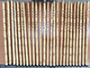 |
Figure 2. The 26 Mansour nay samples used in the study. The arrangement in the photograph is not ordered; sample numbers are defined in Figure 4 and Tables 4 and 7. |
One sample (Sample #01) was subsequently cut transversely and subjected to 3D scanning to obtain detailed internal geometry and wall thickness data (see Sect. 3.1). Since the sound measurements (Sect. 2.2) were completed before this step, all 26 samples have audio recordings. This sample was, however, no longer available for experimental modal analysis; consequently, 25 samples remained for the work described in Section 2.3.
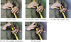 |
Figure 3. Playing Mansour nay to get pitch frequencies. |
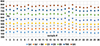 |
Figure 4. The variation of pitch frequencies among the 26 samples. |
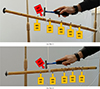 |
Figure 5. Experimental modal test under free boundary conditions. *S: set, **O: output. |
2.2. Sound measurements
Microphone signals were acquired in WAV format from all 26 playable samples at room temperature (24 ± 1 °C) using a Neumann TLM170R microphone with a cardioid polar pattern and a Roland Rubix 22 audio card. The cardioid pattern suppresses background noise and room reflections. The performer played the complete scale of the Mansour nay, G4, A4, B4, C5, D5, E5, F♯5, and G5, at a blowing angle of approximately 30° (Fig. 3). The blowing angle, defined as the angle between the performer’s head and the body of the nay, is one of the first elements taught during conservatory training, and experienced performers maintain it with considerable consistency through muscle memory. Nevertheless, angular variations of up to ±5° were observed when transitioning between notes. Multiple recordings were taken from each sample, and average values were retained in order to reduce the effect of systematic errors. An audio recording of the performance is provided as https://acta-acustica.edpsciences.org/10.1051/aacus/2026050/olm.
 |
Figure 6. Finite element model of the musical instrument. |
Material values used in the computational model of the Mansour nay. For Arundo donax, EL and density are the parameters calibrated by the sequential SOL 200 update on Sample #01; the remaining orthotropic constants are retained from the literature starting values.
The pitch frequencies were extracted from the audio recordings using MakamBox [26], an open-source pitch analysis tool developed for maqam music traditions. The fingering positions and corresponding maqam note names are illustrated in Figure 3; interested readers are referred to [8, 9] for details on the Turkish pitch system. The variation of pitch frequencies across the 26 samples is depicted in Figure 4. Each data point represents the mean pitch frequency of a given note for a given sample, and the spread across samples provides a first visual indication of the inter-specimen variability that is analysed quantitatively in Section 5. The Mansour nay is used both as a solo instrument and in ensemble with other Turkish art music instruments, where it must blend with instruments tuned to a fixed pitch reference. Absolute pitch accuracy is therefore a relevant quality criterion, and the pitch frequencies reported in this paper are interpreted as absolute frequencies rather than only as relative intervals.
2.3. Experimental modal analysis
Experimental modal analysis (EMA) was performed on all 25 playable samples. Prior to the experiments, a pre-test computational model was prepared to determine the optimal sensor and excitation locations. The critical output (accelerometer) locations were identified using the Min-MAC algorithm [27], which minimises the off-diagonal terms of the modal assurance criterion (MAC) matrix. The optimal excitation locations were determined using the normal mode indication function (NMIF) [28]. For the Mansour nay geometry, the Min-MAC algorithm yielded 10 output locations and the NMIF yielded 2 input locations, resulting in a multi-input multi-output (MIMO) experimental configuration with 20 degrees of freedom.
Experimental raw data were acquired using an 8-channel Sinus Soundbook mobile analyser, Dytran 3035BG miniature accelerometers, and a Dytran 5800B3 impact hammer. Due to the limited number of acquisition channels, the measurements were performed in two sets (Fig. 5). In Set 1, five accelerometers were placed along one generating line of the nay body; in Set 2, they were repositioned at a 90° offset around the circumference. The use of five accelerometers per set is the minimum number required to observe at least five bending modes with reliable spatial discrimination along the instrument axis; the corresponding added mass is taken into account in the model updating procedure described in Section 3.2. This arrangement ensures that bending modes in two orthogonal planes are captured. All tests were carried out under free boundary conditions, realised by suspending each instrument with thin wires (Fig. 5). Modal parameters, namely eigenfrequencies, eigenvectors, and damping ratios, were extracted from the measured frequency response functions (FRFs) using Brüel & Kjær nCode software.
The mass of the attached accelerometers alters the natural frequencies of the structure, and this effect differs between the two sets owing to the change in sensor positions. This mass loading effect is accounted for in the model updating procedure described in Section 3.2.
3. Computational modelling
3.1. Finite element model and 3D scanning
Sample #01 was cut transversely at each internode and subjected to 3D scanning to obtain accurate internal and external geometry, including wall thickness data. The resulting CAD model was imported into Siemens Simcenter 3D (version 2312), which is built on NX and employs MSC Nastran solvers.
The Mansour nay consists of four components (Fig. 6): a one-piece 9-internode giant reed body, a Delrin mouthpiece, and two nickel silver bracelets. Giant reed is modelled as an orthotropic material, whereas Delrin and nickel silver are treated as isotropic. The initial mechanical properties of all three materials are summarised in Table 1; those for giant reed were compiled from the literature [6, 7, 29, 30], while those for Delrin and nickel silver were taken from a materials property database [31]. The mesh size was determined through a convergence study using the fundamental frequency from normal mode analysis (Nastran SOL 103) as the convergence criterion. The final model comprises 236 463 elements and 479 112 nodes.
3.2. Model updating
The FE model of Sample #01 was updated to bring the computed eigenfrequencies into agreement with the experimentally measured values from EMA. The update was performed through frequency optimisation using Nastran SOL 200 [32], which in the Simcenter 3D implementation operates on one target eigenfrequency per optimisation run. The procedure was therefore applied sequentially: the first experimental eigenfrequency was set as the target, the optimisation was run, the identified material values were retained, and the procedure was repeated for subsequent eigenfrequencies in ascending order. In each run, the orthotropic mechanical properties of giant reed (elastic moduli, shear moduli, and Poisson’s ratios) were treated as design variables with ±50% bounds on their literature initial values. The mechanical properties of Delrin and nickel silver were held fixed at their literature values [31] throughout the update. The accelerometer masses used in each of the two experimental sets (Sect. 2.3) were included in the corresponding computational models to account for mass loading effects.
It should be noted that not all orthotropic material parameters are identifiable from bending-mode eigenfrequencies alone. The bending behaviour of a thin-walled tube-like structure is governed primarily by the longitudinal Young’s modulus and the density, through the product EI and the mass per unit length; the transverse and radial moduli, the shear moduli, and the Poisson’s ratios have only weak influence on bending-mode frequencies and therefore cannot be identified reliably by an update that uses bending modes as targets. In the present work, EL and the density are the parameters effectively calibrated by the sequential update, and the remaining orthotropic constants are reported close to their literature starting values. The final material values used in the computational model are summarised in Table 1.
3.3. Construction of the Average Mansour Nay Model (AMNM)
The masses, top and bottom outer diameters, wall thicknesses, total lengths, and internode lengths of all 26 samples were measured, a total of 14 geometric variables. Outer diameters were recorded at five locations per internode, giving 42 measurement points per sample.
Since the internal geometry could only be obtained from the single 3D-scanned specimen (Sample #01), a relationship between outer and inner diameter is needed for the remaining 25 samples. Examination of the 3D scan revealed that the wall thickness is approximately constant within each internode but varies from internode to internode. On the basis of this observation, a linear interpolation assumption was adopted: the change from the top inner diameter to the bottom inner diameter is assumed to be linear along the nine internodes. When tested against the true dimensions of Sample #01 (Tab. 2), this assumption yields an average error of 2.42% for the outer diameter and 2.88% for the inner diameter, which was considered acceptable for the purposes of constructing a representative average geometry (Fig. 7).
Outer and inner diameter measurements of the internodes of Sample #01 in millimetres.
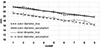 |
Figure 7. Diameter changes at the internodes of Sample #01; comparison of true and assumed values. |
Using this assumption, the internal geometries of all 26 samples were estimated. The average values of all 14 geometric variables were then computed, and the CAD geometry of Sample #01 was modified by substituting these average dimensions. The resulting model is referred to as the Average Mansour Nay Model (AMNM). The maximum, minimum, and average values of the 14 variables across all samples are shown in Figure 8.
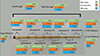 |
Figure 8. Maximum, average, and minimum values of the variables determined in the samples. |
The AMNM does not correspond to any physical specimen; it is a synthetic model whose geometry represents the central tendency of the population. When used as a reference in the stochastic analysis (Sect. 4), the deviation of each physical sample from the AMNM constitutes the “error” whose sources are to be identified.
The AMNM was imported into Simcenter 3D, and the same structural and acoustic analyses described above were repeated. For the model update of the AMNM, Sample #22 was selected as the reference dataset because it exhibited the lowest median deviation from the AMNM eigenfrequencies across all eight modes within the analysis bandwidth. The update was again performed with Nastran SOL 200, adjusting the orthotropic properties of giant reed to match the measured eigenfrequencies of Sample #22 while preserving the average geometry. After updating, the agreement between computed and experimental eigenfrequencies was within 1%.
3.4. Vibroacoustic model
For the acoustic response of the instrument, an acoustic finite element model incorporating fluid–structure interaction (FSI) at the giant reed body and the internal air cavity was constructed. A one-way (weak) coupling approach was adopted, in which the structural vibrations of the giant reed body can in principle affect the internal acoustic field, but the acoustic pressure in the cavity does not feed back to the structure. For a straight, narrow-bore woodwind such as the nay, this simplification is justified on physical grounds. The internal acoustic pressure field is predominantly one-dimensional along the bore axis and essentially axisymmetric in the cross-section, while the lowest wall-vibration modes of a thin-walled tube are bending modes with a cos(θ) or sin(θ) angular dependence. The inner product between an axisymmetric pressure field and a non-axisymmetric wall displacement vanishes at leading order, so pressure-driven wall motion is a higher-order effect and its feedback on the internal acoustic field is negligible, a property well established for tube-like woodwinds such as the clarinet and flute [10].
The frequency-domain simulation is driven by a dipole sound source located at the mouthpiece [10], representing the lateral airstream excitation produced by the performer at the blowing edge. For an end-blown flute such as the nay, the player directs a thin air jet across the mouthpiece opening; this jet oscillation acts on the air column through the flow–pressure asymmetry at the embouchure rather than through a net volume source, and is therefore more accurately represented by a dipole than by a monopole source. A more physically complete representation of the jet–edge interaction would require a nonlinear and player-specific model, which is outside the scope of the present study. The dipole representation is a standard first-order approximation for the excitation of end-blown flutes [10] and is sufficient for the purpose of capturing relative pitch-frequency variation across samples, which is the focus of the uncertainty quantification. The resulting model can be regarded as a linear passive resonator that cannot produce sound unless excited by an external source. The solver employed for the acoustic analysis is Nastran SOL 111.
In playing conditions, the internal acoustic cavity communicates with the ambient air through the open finger holes and the open end of the instrument. A zero acoustic pressure boundary condition is applied at each of these openings, which corresponds to neglecting the radiation impedance of the open holes and of the open end. This approximation is known to produce a small systematic underprediction of the resonance frequencies in absolute terms, because the radiation impedance would otherwise introduce a small end correction that shifts each resonance upward. In the present study, however, this systematic error is applied identically to the AMNM reference and to all 26 sample simulations, so it cancels in the specimen-to-specimen deviations that constitute the training data for the PCE-Kriging surrogate. The variable rankings obtained in Section 5 are therefore unaffected by the end-correction simplification.
Since the set of open holes changes for each note, a separate analysis was performed for each of the five distinct fingering configurations (Fig. 9): (a) G4 (rast), all holes closed; (b) A4, E5 (dugah, huseyni), one hole open; (c) B4, F♯5 (segah, evic), two holes open; (d) C5, G5 (çargah, gerdaniye), three holes open; (e) D5 (neva), five holes open.
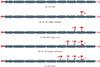 |
Figure 9. Acoustic response analysis of the acoustic model to obtain pitch frequencies for each fingering configuration. The arrows indicate the locations at which boundary conditions are imposed: the dipole source at the mouthpiece and the zero acoustic pressure condition at the open finger holes and the open bottom end. The structural part of the model is hidden for clarity. |
The pitch frequencies produced by the computational model were measured through a virtual microphone placed at the bottom opening of the instrument. The bottom opening is the dominant radiation region for fingering configurations with few holes open, because it is the terminal open end of the tube where the acoustic pressure field has its strongest gradient with respect to the external air. For configurations with multiple holes open, such as the D5 (neva) configuration with five holes open, the open holes also contribute to the radiated field, but the bottom-opening signal remains the primary observable and was retained throughout the analysis for consistency across configurations.
The bore of the instrument exhibits natural narrowing at the internode boundaries (visible in Fig. 9), which reflects the actual internal anatomy of the giant reed. These constrictions are preserved in the model and influence the resonance frequencies.
4. Uncertainty quantification via PCE-Kriging
The goal of the uncertainty quantification (UQ) analysis is to identify which geometric variables of the Mansour nay are the dominant sources of the discrepancies between the AMNM predictions and the experimentally measured frequencies across the 26 samples. To this end, a surrogate model is constructed using polynomial chaos expansion combined with Kriging (PCE-Kriging) [23–25]. This section describes the formulation of the surrogate model, the selection of input variables and their probability distributions, and the validation procedure. All computations were performed in MATLAB using the UQLab framework [33].
4.1. Problem formulation
Let x = (x1, x2, …, xM) denote the vector of M geometric input variables characterising a given Mansour nay sample (e.g. top diameter, bottom diameter, mass, internode lengths, finger hole distances) and let y denote a scalar response quantity of interest, either a structural eigenfrequency or an acoustic pitch frequency. For each sample, the response of the AMNM, denoted  , is computed using the finite element model described in Section 3. The discrepancy between the computed and experimentally measured response is defined as the error
 (1)
(1)
which serves as the dependent variable (output) of the surrogate model. The objective is to express this error as a function of the input variables, e ≈ f(x), and thereby to determine which inputs contribute most to the observed variability.
4.2. Polynomial chaos expansion
Polynomial chaos expansion (PCE) is a spectral method that approximates a computational model by projecting its output onto a basis of orthogonal polynomials [23]. For a model with M stochastic input variables, the PCE representation of the output is written as
 (2)
(2)
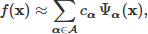
where cα are the expansion coefficients, Ψα(x) are multivariate orthogonal polynomials constructed as products of univariate polynomials, α is a multi-index indicating the polynomial degree in each variable, and 𝒜 is the set of retained multi-indices. The univariate polynomial families are chosen to be orthogonal with respect to the marginal probability distribution of each input variable; for instance, Hermite polynomials correspond to Gaussian distributions, and Jacobi polynomials correspond to Beta distributions [33]. A sparse truncation scheme is adopted so that only those polynomial terms whose total degree does not exceed a prescribed maximum (typically p = 3) are retained. This keeps the number of unknown coefficients manageable relative to the available sample size.
PCE captures the global trend of the model response as a function of the input variables.
4.3. Kriging
Kriging is a Gaussian-process-based interpolation method that models the output as the sum of a deterministic trend function and a stochastic residual [24]:
 (3)
(3)
where μ(x) is the trend (or mean) function and Z(x) is a zero-mean Gaussian process characterised by a covariance function (kernel). The covariance function encodes assumptions about the smoothness and correlation structure of the residual. Kriging provides not only a point prediction at any untried input but also an estimate of the prediction uncertainty, which is particularly valuable when the number of training points is small.
4.4. PCE-Kriging
PCE-Kriging combines the strengths of both methods: PCE provides a global polynomial approximation of the model response, and Kriging interpolates the local deviations that the polynomial cannot capture [23–25]. In practice, the construction proceeds in two steps. First, the optimal set of polynomial basis functions for the PCE is identified using a sparse regression algorithm (least-angle regression, LAR). Second, the selected polynomial basis is used as the trend function μ(x) in the Kriging model, and the Kriging hyperparameters (correlation lengths and variance) are calibrated by maximum likelihood estimation. The resulting surrogate model can be written as
 (4)
(4)
This hybrid formulation is particularly suited to the present problem for two reasons. First, the dataset is small (26 samples), which limits the applicability of purely data-driven methods that require large training sets. PCE-Kriging has been shown to outperform standalone PCE and standalone Kriging on small datasets because the polynomial trend captures the dominant global behaviour while the Kriging component accounts for residual local variations [23, 24]. Second, the orthogonal polynomial basis of the PCE component allows the relative importance of each input variable to be assessed directly through the expansion coefficients, without requiring additional sensitivity analyses.
4.5. Two-model workflow and definition of observables
The PCE-Kriging framework introduced in Section 4.1 is applied to two distinct modelling problems in this study. The two problems share the same set of candidate geometric input variables and the same surrogate modelling procedure, but they differ in the physical observable used as the model output and in the computational model from which the reference values are obtained.
In the acoustic model, the observable is the pitch frequency of each played note, obtained from audio recordings of a professional performer (Sect. 2.2). The reference value for each note is the pitch frequency predicted by the vibroacoustic finite element model applied to the AMNM geometry (Sect. 3.4). The discrepancy between the AMNM prediction and the measured pitch, taken across the 26 samples and the five fingering configurations, constitutes the error vector that the surrogate model is trained to reproduce. The acoustic model therefore characterises the inter-specimen variability of the pitch frequencies produced by the instrument under performance conditions.
In the structural model, the observable is the eigenfrequency of each bending mode within the analysis bandwidth, obtained from experimental modal analysis under free boundary conditions (Sect. 2.3). The reference value for each mode is the eigenfrequency predicted by the structural finite element model of the AMNM geometry (Sect. 3.2). The discrepancy between the AMNM prediction and the measured eigenfrequency, taken across the 25 samples and the eight bending modes, constitutes the error vector for this case. The structural model therefore characterises the inter-specimen variability of the free-structure dynamics of the instrument, and, as discussed in the introduction and in Section 5.3, is reported here as a methodological demonstration of the PCE-Kriging framework rather than as a musically relevant finding.
In both cases, the candidate geometric variables measured for the samples form the input space, and the surrogate modelling procedure of Sections 4.1–4.4 is applied independently to each problem. The ranking of input variables obtained from the two models may therefore differ, and any difference reflects the distinct physical mechanisms by which the geometric variables affect each observable.
4.6. Input variables and probability distributions
The 14 geometric variables measured for each of the 26 samples (Sect. 3.3) form the candidate input set for the structural model. Before constructing the surrogate model, a preliminary screening was performed to identify variables that vary systematically across the sample population. Nonparametric rank-based tests (including Kruskal–Wallis) were applied to each variable using geographic region and cutting year as grouping factors. The full screening results are presented in Table 3. At the 5% significance level by geographic region, four variables pass the screening: bottom diameter (p = 0.034), mass (p = 0.048), and the lengths of internodes 5 (p = 0.015) and 6 (p = 0.037). No variable shows statistically significant variation by cutting year.
Screening of candidate geometric variables for the structural model. The Kruskal–Wallis test was applied to each of the 14 variables to test for differences across the four geographic regions and the three cutting years of the sample population. Bold p-values indicate statistical significance at the 5% level.
Comparison of computed pitch frequencies of the AMNM and the pitch frequencies derived from audio recordings of 26 samples (in Hz).
Of these four retained candidates, the bottom diameter and the mass were selected as stochastic inputs for the PCE-Kriging surrogate model. This choice reflects the physics of a thin-walled tapered tube: the bending eigenfrequencies of the instrument depend primarily on the cross-sectional stiffness and the mass per unit length, both of which are captured by these two variables. The individual internode lengths contribute to the eigenfrequencies primarily through their collective effect on the total length and the distributed mass, which are already represented through the total length and the mass, respectively.
For each retained variable, the most appropriate parametric probability distribution was fitted to the measured data using maximum likelihood estimation. The choice of distribution family (Gaussian, Student-t, Gumbel, Beta, etc.) was guided by the empirical distribution shape and confirmed by goodness-of-fit tests. The fitted distributions and their moment parameters are reported alongside the results in Section 5.
When two or more input variables are correlated, as is the case, for example, with the bottom diameter and mass, the statistical dependence is modelled through a copula function. Specifically, the Clayton copula
 (5)
(5)
was employed, where u1 and u2 are the marginal cumulative distribution function values of the two variables. The copula parameter θ was estimated from the data and accounts for the lower-tail dependence between the correlated variables.
4.7. Surrogate model coefficients and interpretation
Once the PCE-Kriging model is constructed, the expansion coefficients cα in equation (4) quantify the contribution of each polynomial term, and hence each input variable or combination of variables, to the total error. These are unstandardised regression coefficients: a larger absolute value of cα indicates a stronger influence of the corresponding variable (or variable interaction) on the discrepancy between the AMNM and the experimental data. By examining which coefficients are dominant, the variables that drive the inter-specimen variability can be ranked. It should be noted that a large coefficient indicates statistical influence on the modelled observable but does not automatically imply a practically relevant perceptual consequence; the interpretation of the coefficients in terms of their practical significance is deferred to Section 5.3.
4.8. Model validation
The predictive accuracy of the surrogate model is assessed through leave-one-out (LOO) cross-validation [33]. In this procedure, the model is trained on N − 1 samples and used to predict the response of the excluded sample; this is repeated for each of the N samples, and the average prediction error is computed. The LOO error provides an unbiased estimate of the generalisation performance without requiring a separate validation dataset, which is important given the limited sample size.
5. Results and discussion
This section presents the results of the PCE-Kriging analysis described in Section 4, applied first to the acoustic pitch frequencies (Sect. 5.1) and then to the structural eigenfrequencies (Sect. 5.2), which are reported as a methodological case study. The practical implications of the findings are discussed in Section 5.3.
5.1. Uncertainty quantification in the acoustic model
Before presenting the uncertainty quantification results, it is useful to recall the first-order physics of the pitch frequencies. The Mansour nay is an open-ended wind instrument: the top is an open blowing edge at which the acoustic pressure is at (or close to) atmospheric, and the bottom is the open end of the tube. To a first approximation, the playable resonance frequencies of such an open–open tube are given by
 (6)
(6)
where c is the speed of sound in air, n is the mode index, Leff is the effective acoustic length from the blowing edge to the first open finger hole (or to the bottom opening when all holes are closed), and Δ is the combined end correction from the two open ends, which depends on the bore diameter. For a thin-walled tube of internal radius r, each open end contributes an end correction of approximately 0.6 r to the acoustic length. Consequently, pitch frequencies depend most strongly on the effective length Leff, which in turn is controlled by the position of the first open finger hole and by the total length of the nay; and they depend, through the end correction Δ, on the bore diameter. This simple picture anticipates the two most important outcomes of the uncertainty quantification reported below: the top and bottom diameters, through their effect on the end correction, emerge as dominant contributors to the observed pitch variability, and the finger hole distances, through their effect on Leff, emerge as the next most important group of variables.
The AMNM was subjected to acoustic response analysis using Nastran SOL 111 to compute the reference pitch frequencies, as described in Section 3.4. The five vibroacoustic models with different boundary conditions (Fig. 9) yield the acoustic response curves shown in Figure 10. The second peaks in each response curve correspond to the fundamental pitch frequencies: G4 (rast, 380 Hz), A4 (dugah, 432 Hz), B4 (segah, 486 Hz), C5 (çargah, 518 Hz), and D5 (neva, 586 Hz). The third peaks of the dugah, segah, and çargah models correspond to the register pitches E5 (huseyni, 642 Hz), F♯5 (evic, 720 Hz), and G5 (gerdaniye, 764 Hz), respectively.
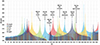 |
Figure 10. The computed pitch frequencies of the AMNM. The dB scale shown is relative to the default internal reference of the Simcenter acoustic solver. |
The named notes in Figure 10 correspond to the second mode of the tube for the all-closed G4 (rast) configuration and to progressively higher modes for configurations with open holes. The fundamental mode of the all-closed tube, which lies approximately one octave below G4, is not conventionally played and is not labelled; additional resonance peaks visible in Figure 10 correspond to tube resonances that fall outside the Turkish music scale and are not part of the standard repertoire. An experienced performer can nonetheless produce the fundamental by reducing blowing pressure and adjusting embouchure, which provides a potential direction for future experimental validation.
The comparison of computed AMNM pitch frequencies and the pitch frequencies derived from audio recordings of the 26 samples is given in Table 4.
For the acoustic model, the candidate input variable set is larger than for the structural model because the finger hole distances now directly affect the acoustic resonance frequencies. The variables considered are: mass, total length, top diameter, bottom diameter, and the six finger hole distances (4/26, 5/26, 6/26, 8/26, 9/26, and 10/26), giving a total of 10 input variables.
To reduce the dimensionality while preserving the information content, a factor analysis was performed. The rotated factor analysis with a statistically accepted explained variance of 0.84 shows that the 10 variables can be grouped into five factors:
(i) Factor 1: distances between the finger holes, except 4/26; (ii) Factor 2: top diameter; (iii) Factor 3: bottom diameter and mass; (iv) Factor 4: total length; (v) Factor 5: the distance between finger hole 4/26 and the bottom diameter.
The probability distributions of these five factors, fitted using UQLab [33], are given in Table 5.
Probability distributions of the five factors (acoustic model).
PCE-Kriging expansion coefficients (acoustic model).
Comparison of computational eigenfrequencies of the AMNM and experimental eigenfrequencies of 25 samples (in Hz).
The PCE-Kriging model was constructed with these five factors as inputs and the pitch frequency errors (differences between AMNM computed values and audio-recorded values) as the output. The LOO cross-validation error is 0.32 Hz, confirming that the surrogate model predicts the pitch frequency discrepancies with high accuracy.
The expansion coefficients of the PCE-Kriging model are given in Table 6. The coefficients indicate the following ranking of variable importance, from highest to lowest impact: (1) Top diameter (Factor 2, coefficient =9.98) and bottom diameter + mass (Factor 3, coefficient =9.98), equally dominant; (2) Finger hole distances except 4/26 (Factor 1, coefficient =4.35); (3) Total length (Factor 4, coefficient =3.58); (4) Distance of finger hole 4/26 and bottom diameter (Factor 5, coefficient =0.07), negligible.
5.2. Uncertainty quantification in the structural model: a methodological case study
The same PCE-Kriging framework applied to the acoustic observable in Section 5.1 is now applied to the structural observable defined in Section 4.5, namely the bending eigenfrequencies of the instrument under free boundary conditions. The purpose of this subsection is methodological rather than acoustic. As discussed in the introduction, the coupling between wall bending vibrations and the internal air column is negligible for a straight, narrow-bore woodwind, and the free-boundary eigenfrequencies reported here therefore do not correspond to a musically audible effect of the nay in performance. They are nevertheless useful for two reasons. First, they provide an independent test of the PCE-Kriging framework on a second observable computed from the same sample set, which allows the robustness of the surrogate modelling approach to be assessed on a dataset of the same small size. Second, the ranking of geometric variables that emerges from the structural analysis is of physical interest in its own right, and it demonstrates how the framework would be applied to an instrument for which wall vibration is musically significant, such as a string instrument soundbox or a percussion body.
The eigenfrequencies of the AMNM, computed using Nastran SOL 103 after the model update described in Section 3.3, are compared with the experimentally measured natural frequencies of the 25 samples in Table 7. All eight modes within the analysis bandwidth are bending modes that appear sequentially about two orthogonal planes (y and z) perpendicular to the instrument axis (x). Due to the nearly axisymmetric geometry, bending modes occur in pairs at slightly different frequencies: modes 1–2 constitute the first bending pair, and modes 3–4 the second. The third bending pair appears to correspond to modes 6 and 7, whose frequencies are close in both the AMNM prediction (760 Hz and 779 Hz) and the experimental measurements. Mode 5, at 694 Hz in the AMNM, does not fit the regular bending-pair sequence and is most likely a different mode type, possibly a bending–torsion coupled mode or a higher-order lateral mode, rather than a companion of mode 6. Mode 8 is the fourth bending pair. The mode shapes of the AMNM are shown in Figure 11.
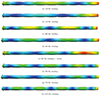 |
Figure 11. The mode shapes of the AMNM. |
A systematic discrepancy should be noted for mode 7. The AMNM prediction of 779 Hz lies substantially below the experimental values, which range from 939 Hz to 1154 Hz across the 25 samples, corresponding to relative differences of 21% to 48%. All other modes show relative differences within approximately 9% to 18%. This pattern is not consistent with a simple specimen-to-specimen variability and suggests instead that the numerical and experimental modes identified as “mode 7” may not correspond to the same physical mode shape. Closely spaced modes in a nearly axisymmetric structure are difficult to pair reliably by frequency ordering alone, and a rigorous pairing would require a modal assurance criterion between computed and measured mode shapes, which was not performed in this study. The mode 7 data point is therefore included in Table 7 for completeness and contributes to the PCE-Kriging training together with the other modes, but the reader is cautioned that its contribution to the surrogate model may reflect a pairing artefact rather than a physical variability. As discussed in Section 5.3, the structural analysis is in any case reported as a methodological demonstration rather than as a musically relevant finding.
The discrepancy between the AMNM eigenfrequencies and the experimental values of each sample constitutes the error vector used in the PCE-Kriging model. The screening of the 14 candidate geometric variables described in Section 4.6 (Tab. 3) identified bottom diameter and mass as the two variables retained as stochastic inputs on physical grounds. The finger hole locations were examined separately. The descriptive statistics of the finger hole distances are given in Table 8. Spearman’s rank correlation coefficients between the finger hole distances range from 0.83 to 0.97, indicating that all six finger hole positions are highly correlated. The Kruskal–Wallis test showed no statistically significant difference in finger hole locations according to either geographic origin or cutting year at the 5% level, confirming that the professional luthier’s drilling process introduces negligible variation.
Descriptive statistics of finger hole locations (in cm).
The note with the highest positional variation is G4 (rast, position 26/26), which is expected because this is the full tube length; it is not controlled by a drilled hole but by the natural length of the reed and the position of the bottom end.
The bottom diameter and mass are modelled as random variables and their probability distributions are fitted using UQLab [33] and MATLAB. The fitted distributions and their moment parameters are given in Table 9. The statistical dependence between the two variables is modelled through the Clayton copula defined in Section 4 (Eq. (5)).
Probability distributions of statistically significant variables (structural model).
The PCE-Kriging surrogate model was then constructed with these two input variables and the eigenfrequency errors as the output. The leave-one-out (LOO) cross-validation error of the model is 0.08 Hz, indicating excellent predictive accuracy. The expansion coefficients of the surrogate model are given in Table 10. The bottom diameter has a substantially larger coefficient (1.40) than the mass (0.05), indicating that it is the dominant source of the discrepancy between the AMNM eigenfrequencies and the experimentally measured values. This result is physically intuitive: the bottom diameter directly governs the internal cross-sectional area at the wider end of the instrument, which strongly affects both the structural stiffness distribution and the enclosed air volume.
PCE-Kriging expansion coefficients (structural model).
5.3. Discussion
The results of Sections 5.1 and 5.2 can be interpreted from both a physical and a practical standpoint.
For the acoustic model, the top and bottom diameters emerge as the most influential variables, with equal coefficients. This can be understood from the acoustic perspective: the bore profile, characterised by the taper from the top (mouthpiece end) to the bottom (open end), is the primary determinant of the resonance frequencies of the air column. The top diameter governs the input impedance at the excitation point, while the bottom diameter governs the radiation impedance at the open end. Their combined effect on the resonance frequencies exceeds that of the finger hole positions (Factor 1), which are themselves the third most important variable group. The total length (Factor 4) has a moderate effect, while the distance of finger hole 4/26 and the bottom diameter (Factor 5) is negligible.
For the structural model, the dominance of the bottom diameter is consistent with the mechanics of a tapered cylindrical shell: the wider end contributes disproportionately to the bending stiffness and to the enclosed mass of air, and small variations in this dimension propagate to all modal frequencies. The mass, while statistically significant, has a much smaller coefficient, suggesting that its effect on the eigenfrequencies is secondary.
Several limitations of the present study should be acknowledged explicitly. First, the experimental modal analysis was performed under free boundary conditions, whereas in performance the instrument is held by the player, which modifies the boundary conditions, adds damping, and alters the observability of individual modes. The structural eigenfrequencies reported here therefore characterise the instrument as a free structure and should not be interpreted as properties of the played instrument. As discussed in the introduction, the coupling between wall vibration and the internal air column is negligible for a straight, narrow-bore woodwind, and the structural results in Section 5.2 are presented as a methodological demonstration of the PCE-Kriging framework rather than as acoustically relevant findings. The framework itself is transferable to instruments where wall vibration does play a musically significant role, such as string instrument soundboxes or percussion bodies.
Second, the pitch frequencies used as the acoustic observable were extracted from recordings of a professional performer playing each instrument, rather than from input impedance measurements of the resonator alone. The played pitch reflects the combined response of the instrument, the player’s embouchure, blowing pressure, and any compensation the performer applies. This is appropriate for the practical question addressed in this study, namely which geometric variables produce perceptible pitch differences across instruments that are about to be delivered to performers. It is not equivalent to a characterisation of the acoustic resonator in isolation. All recordings were carried out at a controlled room temperature of 24 °C ± 1 °C with a single experienced performer, which minimises inter-performer variability but does not eliminate the performer’s contribution to the measured pitch.
Third, the study focuses on geometric sources of variability and does not quantify the acoustic consequences of material properties. As noted in the introduction, material effects such as internal surface roughness, porosity, and hygroscopic behaviour during play are expected to influence viscothermal losses and therefore timbre and playability, but these fall outside the scope of the present work. The practical recommendations that follow are formulated in terms of geometric parameters that the instrument maker can assess and control at the reed-selection and finger-hole-drilling stages.
A sensitivity analysis was performed to verify that the variable ranking obtained in Sections 5.1 and 5.2 is not an artefact of the absolute-error definition adopted in equation (1). The analysis was repeated with the relative error  substituted for the absolute error, using a polynomial-regression surrogate on the same input set and the same error outputs. The Spearman rank correlation between the two rankings is essentially unity for both the acoustic and the structural models, and the three most influential variables are unchanged in both cases. The variable ranking is therefore insensitive to the choice between absolute and relative error. We note further that the variation ranges analysed in this study arise from the specific population of Arundo donax samples examined and characterise the material population within the instrument, not the instrument concept in a universal sense.
From a practical perspective, the acoustic findings provide quantitative guidance for instrument makers. In the reed selection stage, giant reeds with comparable top and bottom diameters are expected to produce instruments with more consistent pitch behaviour, since these two variables together account for the largest share of the observed pitch variability. In the subsequent finger hole drilling stage, the linear bore assumption introduced in Section 3.3 provides a practical route for estimating the internal bore profile from external calliper measurements alone, which is directly applicable in the workshop. These recommendations address geometric variability only; effects attributable to the acoustic properties of Arundo donax itself, such as internal surface roughness, porosity, and hygroscopic behaviour during play, are recognised as relevant to timbre and playability but fall outside the scope of the present work and remain an open direction for future study.
The finding that finger hole 4/26, the hole closest to the open end, has negligible influence on pitch frequency variation is noteworthy. This hole produces the note G4 (rast), which corresponds to the full effective tube length and is known to exhibit the largest pitch variation across samples (Tab. 8). The G4 pitch is governed primarily by the overall tube geometry rather than by the hole position, which explains why variations in the 4/26 distance do not propagate to the other pitches. Additionally, the formation of extra internode knots near the bottom end of some aged reeds [34] further increases the variability of this particular note. In performance practice, performers routinely tune the G4 note by adjusting the embouchure, which is consistent with the observation that this note is inherently less stable than the others.
6. Conclusion
This study has investigated the geometric sources of variability in 26 Mansour nay samples by combining audio-based pitch measurements, vibroacoustic finite element modelling, and uncertainty quantification through PCE-Kriging surrogate modelling. The Average Mansour Nay Model (AMNM), constructed from the measured geometric properties of all samples, serves as the reference against which specimen-to-specimen deviations are quantified.
The principal acoustic finding is that the top diameter and the bottom diameter of the bore, together with the mass, are the dominant geometric contributors to pitch frequency variability across instruments. Their combined influence exceeds that of the finger hole distances, which rank third, followed by the total length. The PCE-Kriging model achieves a leave-one-out cross-validation error of 0.32 Hz on the pitch frequency discrepancies, which confirms the predictive accuracy of the surrogate model on this small dataset.
As a methodological demonstration, the same PCE-Kriging framework was applied to the structural eigenfrequencies of the instrument measured under free boundary conditions. The bottom diameter and mass emerge as the statistically significant variables in this case, with a leave-one-out error of 0.08 Hz. These structural results are reported as a case study of the uncertainty quantification approach rather than as musically relevant findings, since the coupling between wall vibration and the internal air column is negligible for a straight, narrow-bore woodwind. The framework itself is transferable to instruments where wall vibration is musically significant, such as string instrument soundboxes or percussion bodies.
For instrument makers, the acoustic findings translate into practical guidance at two stages of nay making. At the reed-selection stage, giant reeds with comparable top and bottom diameters are expected to produce instruments with more consistent pitch behaviour, since these two variables together account for the largest share of the observed pitch variability. At the finger-hole-drilling stage, the linear bore assumption introduced in Section 3.3 provides a practical route for estimating the internal bore profile from external calliper measurements, which allows hole positions to be adjusted for the specific geometry of each reed. These recommendations address geometric variability only. Effects attributable to the acoustic properties of Arundo donax itself, such as internal surface roughness, porosity, and hygroscopic behaviour during play, are recognised as relevant to timbre and playability but fall outside the scope of the present work and remain an open direction for future study.
Beyond the specific case of the Mansour nay, the combined vibroacoustic modelling and PCE-Kriging methodology is transferable to other musical instruments made from natural materials where specimen-to-specimen variability is inherent. The approach is particularly suited to small datasets, where purely data-driven methods are constrained by the limited number of training points.
Funding
This study was supported by Scientific and Technological Research Council of Türkiye (TÜBİTAK) under the Grant number 221M499. The authors thank TÜBİTAK for their support.
Conflicts of interest
The authors declare that they have no conflicts of interest in relation to this article.
Data availability statement
Data are available on request from the authors.
Supplementary material
An audio recording of the performance is provided as supplementary material. Access Supplementary Material
References
- Dunn, F., Hartmann, W.M., Campbell, D.M., Fletcher, N.H.: Springer Handbook of Acoustics. Springer, 2015. [Google Scholar]
- Gazengel, B., Dalmont, J.-P.: Mechanical response characterisation of saxophone reeds, in: Proceedings of Forum Acusticum, Aalborg, Denmark, 2011. [Google Scholar]
- Campbell, M., Gilbert, J., Myers, A.: The Science of Brass Instruments. Springer, 2021. [Google Scholar]
- Ribble, D.B.: The shakuhachi and the ney: a comparison of two flutes from the far reaches of Asia. Minutes of Kochi Medical University 19 (2003) 1–13. [Google Scholar]
- Yarkın, N., Tan, A.: A study of the reference pitches in Ottoman-Turkish music through an analysis of historical neys. Ethnomusicology Journal 4, 2 (2021) 273–286. [Google Scholar]
- Akahoshi, H., Obataya, E.: Effects of wet-dry cycling on the mechanical properties of Arundo donax L. used for the vibrating reed in woodwind instruments. Wood Science and Technology 49, 6 (2015) 1171–1183. [Google Scholar]
- Weidenfeller, B., Lambri, O.A., Bonifacich, F.G., Arlic, U., Gargicevich, D.: Damping of the woodwind instrument reed material Arundo donax L. Materials Research 21 (2018) e20170795. [Google Scholar]
- Gedik, A.C., Bozkurt, B.: Evaluation of the Makam scale theory of Arel for music information retrieval on traditional Turkish art music. Journal of New Music Research 38, 2 (2009) 103–116. [Google Scholar]
- Wimmer, B., Gómez, E.: Temporal evolution of Makam and Usul relationship in Turkish Makam. Musicological Annual 58, 2 (2022) 107–119. [Google Scholar]
- Wolfe, J.: The acoustics of woodwind musical instruments. Acoustics Today 14, 1 (2018) 50–56. [Google Scholar]
- Damodaran, A., Mansour, H., Lessard, L., Scavone, G., Babu, A.S.: Application of composite materials to the chenda, an Indian percussion instrument. Applied Acoustics 88 (2015) 1–5. [Google Scholar]
- Quintavalla, M., Gabrielli, F., Canevari, C.: Grading materials for stringed instruments soundboards: an approach considering the orthotropic elastic and damping properties. Applied Acoustics 187 (2022) 108521. [Google Scholar]
- Brezas, S., Katsipis, M., Orphanos, Y., Kaselouris, E., Kechrakos, K., Kefaloyannis, N., Hapadaki, H., Sarantis-Karamesinis, A., Petrakis, S., Theodorakis, I., Iliadis, E.: An integrated method for the vibroacoustic evaluation of a carbon fiber bouzouki. Applied Sciences 13, 7 (2023) 4585. [Google Scholar]
- Brauchler, A., Gonzalez, S., Vierneisel, M., Ziegler, P., Antonacci, F., Sarti, A., Eberhard, P.: Model-predicted geometry variations to compensate material variability in the design of classical guitars. Scientific Reports 13 (2023) 12766. [CrossRef] [PubMed] [Google Scholar]
- Brauchler, A., Hose, D., Ziegler, P., Hanss, M., Eberhard, P.: Distinguishing geometrically identical instruments: possibilistic identification of material parameters in a parametrically model order reduced finite element model of a classical guitar. Journal of Sound and Vibration 535 (2022) 117071. [CrossRef] [Google Scholar]
- Viala, R., Placet, V., Cogan, S.: Model-based evidence of the dominance of the guitar brace design over material and climatic variability for dynamic behaviours. Applied Acoustics 182 (2021) 108275. [CrossRef] [Google Scholar]
- Viala, R., Pérez, M.A., Placet, V., Manjón, A., Foltête, E., Cogan, S.: Towards model-based approaches for musical instruments making: validation of the model of a Spanish guitar soundboard and characterisation features proposal. Applied Acoustics 172 (2021) 107591. [Google Scholar]
- Viala, R., Placet, V., Foltête, E., Cogan, S.: Model based ranking of the influence of geometry and materials on the dynamical behavior of the violin highlights predominance of geometrical choices. Scientific Reports 14 (2024) 29589. [Google Scholar]
- Ernoult, A., Chabassier, J., Rodriguez, S., Humeau, A.: Full waveform inversion for bore reconstruction of woodwind-like instruments. Acta Acustica 5 (2021) 47. [CrossRef] [EDP Sciences] [Google Scholar]
- Noreland, D., Kergomard, J., Laloë, F., Vergez, C., Guillemain, P., Guilloteau, A.: The logical clarinet: numerical optimisation of the geometry of woodwind instruments. Acta Acustica united with Acustica 99 (2013) 615–628. [CrossRef] [Google Scholar]
- Cabaret, J., Dalmont, J.-P., Ernoult, A., Fréour, V., Viala, R.: Creation of an experimental database, for the validation of resonator models, comparison of geometries and materials, and quantification of measurement errors, in: Proceedings of Forum Acusticum, Turin, Italy, 2023. [Google Scholar]
- Couineaux, F., Ablitzer, F., Gautier, F.: Minimal physical model of the cristal Baschet. Acta Acustica 7 (2023) 49. [CrossRef] [EDP Sciences] [Google Scholar]
- Aversano, G., D’Alessio, G., Coussement, A., Contino, F., Parente, A.: Combination of polynomial chaos and Kriging for a reduced-order model of reacting flow applications. Results in Engineering 10 (2021) 100223. [Google Scholar]
- Schöbi, R., Sudret, B., Marelli, S.: Rare event estimation using polynomial-chaos kriging. ASCE-ASME Journal of Risk and Uncertainty in Engineering Systems. Part A: Civil Engineering 3, 2 (2017) D4016002. [Google Scholar]
- Zhou, T., Peng, Y.: Reliability analysis using adaptive polynomial-chaos kriging and probability density evolution method. Reliability Engineering and System Safety 220 (2022) 108283. [Google Scholar]
- Atıcı, B.M., Bozkurt, B.: A culture-specific analysis software for Makam music traditions, in: Proceedings of the Fifth International Workshop on Folk Music Analysis (FMA), Paris, France, 2015. [Google Scholar]
- Li, D.S., Fritzen, C.P., Li, H.N.: Extended MinMAC algorithm and comparison of sensor placement methods, in: Proceedings of IMAC-XXVI, Orlando, FL, USA, 2008. [Google Scholar]
- Allemang, R.J., Phillips, A.W.: Experimental modal parameter evaluation methods, in: R. Allemang, P. Avitabile (Eds.). Handbook of Experimental Structural Dynamics. Springer, 2020. [Google Scholar]
- US Department of Agriculture, Forest Service: Wood Handbook – Wood as an Engineering Material. General Technical Report FPL-GTR-190, Madison, WI, 2010. [Google Scholar]
- Fiore, V., Scalici, T., Valenza, A.: Characterisation of a new natural fiber from Arundo donax L. as potential reinforcement of polymer composites. Carbohydrate Polymers 106 (2014) 77–83. [Google Scholar]
- MatWeb Material Property Data, www.matweb.com (accessed 2025). [Google Scholar]
- Mottershead, J.E., Link, M., Friswell, M.I., Schedlinski, C.: Model updating, in: R. Allemang, P. Avitabile (Eds.). Handbook of Experimental Structural Dynamics. Springer, 2022. [Google Scholar]
- Marelli, S., Sudret, B.: UQLab: a framework for uncertainty quantification in MATLAB, in: Vulnerability, Uncertainty, and Risk: Quantification, Mitigation, and Management. ASCE, 2014, pp. 2554–2563. [Google Scholar]
- Tan, A.: The problem of extra node on the ney instrument. PESA International Journal of Social Sciences 4, 1 (2018) 142–147. [Google Scholar]
Cite this article as: Oktav A. Tan A. & Başaran M.A. 2026. Quantifying the variability in Mansour nay: a stochastic approach combining vibroacoustic modelling and PCE-Kriging. Acta Acustica, 10, 52. https://doi.org/10.1051/aacus/2026050.
All Tables
Material values used in the computational model of the Mansour nay. For Arundo donax, EL and density are the parameters calibrated by the sequential SOL 200 update on Sample #01; the remaining orthotropic constants are retained from the literature starting values.
Outer and inner diameter measurements of the internodes of Sample #01 in millimetres.
Screening of candidate geometric variables for the structural model. The Kruskal–Wallis test was applied to each of the 14 variables to test for differences across the four geographic regions and the three cutting years of the sample population. Bold p-values indicate statistical significance at the 5% level.
Comparison of computed pitch frequencies of the AMNM and the pitch frequencies derived from audio recordings of 26 samples (in Hz).
Comparison of computational eigenfrequencies of the AMNM and experimental eigenfrequencies of 25 samples (in Hz).
Probability distributions of statistically significant variables (structural model).
All Figures
|
Figure 1. The measurement rule applied by luthiers in determining finger hole locations. |
| In the text | |
|
Figure 2. The 26 Mansour nay samples used in the study. The arrangement in the photograph is not ordered; sample numbers are defined in Figure 4 and Tables 4 and 7. |
| In the text | |
|
Figure 3. Playing Mansour nay to get pitch frequencies. |
| In the text | |
|
Figure 4. The variation of pitch frequencies among the 26 samples. |
| In the text | |
|
Figure 5. Experimental modal test under free boundary conditions. *S: set, **O: output. |
| In the text | |
|
Figure 6. Finite element model of the musical instrument. |
| In the text | |
|
Figure 7. Diameter changes at the internodes of Sample #01; comparison of true and assumed values. |
| In the text | |
|
Figure 8. Maximum, average, and minimum values of the variables determined in the samples. |
| In the text | |
|
Figure 9. Acoustic response analysis of the acoustic model to obtain pitch frequencies for each fingering configuration. The arrows indicate the locations at which boundary conditions are imposed: the dipole source at the mouthpiece and the zero acoustic pressure condition at the open finger holes and the open bottom end. The structural part of the model is hidden for clarity. |
| In the text | |
|
Figure 10. The computed pitch frequencies of the AMNM. The dB scale shown is relative to the default internal reference of the Simcenter acoustic solver. |
| In the text | |
|
Figure 11. The mode shapes of the AMNM. |
| In the text | |
Current usage metrics show cumulative count of Article Views (full-text article views including HTML views, PDF and ePub downloads, according to the available data) and Abstracts Views on Vision4Press platform.
Data correspond to usage on the plateform after 2015. The current usage metrics is available 48-96 hours after online publication and is updated daily on week days.
Initial download of the metrics may take a while.