© The Author(s), Published by EDP Sciences, 2023

1 Introduction

One of the big challenges for sound reinforcement is to provide high-quality sound for the largest parts of a predefined audience area [1]. High-quality, high-power supply of large audience areas with consistently reinforced sound pressure levels has been considering line-source loudspeaker arrays driven by identical signals for several decades, nowadays. The wavefront sculpture technology (WST [2, 3]) as contemporary line-source theory is based on adjusting the length of the most relevant, binary Fresnel zone for all distances from the stage. Despite the simplicity of its model and a handful of criteria it needs, it provides a powerful and practical theory for line-source loudspeaker arrays. Furthermore, Straube et al. [4, 5], Hölter et al. [6] and Thompson et al. [7–9] discuss the modeling and optimization of the line-source array curvature to obtain tilt angles between the discrete elements, adapted to the listening area. Line-source arrays could also be applied in surround sound applications, and for instance Toole [10] of p. 330 describes the application of line sources compared to point-source loudspeaker setups.

As an alternative way to obtain a desired sound level curve over the listening area, beamforming based on constrained least square optimization was suggested by Beuningen et al. [11]. Beamformers can be found in applications with microphone arrays [12] and with loudspeaker arrays [13–15], and they require individual delays and amplification per transducer, often also filtering.

Moreover, delay and sum beamformers, or phased arrays as they are called when used for narrow-band signals, are also found in antenna theory, radar applications, or optics [16–18]. For a linear antenna array, Shanks [19] applied the stationary phase approximation to determine from the array’s radiation integral the phase and amplitude function required to form a cosecant-squared beam. Chiang et al. [20] used the same approximation method to estimate the beampatterns of in-phase curvilinear arrays, and Chakraborty et al. [21] applied the approximation to a linear array, obtained and solved a first-order differential equation, e.g., to form a cosecant beam. The cosecant beam is equivalent to a 0 dB attenuation target per doubling of the distance, when employing a vertical array below/above a horizontal plane.

Stationary-phase approximation has not only proven to be a powerful tool in antenna beamforming, but it is also used in wave field synthesis [22–24] and yields relatively simple signal processing (gains, delays, common pre-filter). What is more, Schultz [25] suggested the Fourier transform and wave field synthesis as theoretical background for line-source loudspeaker arrays.

In cinema sound practice, SMPTE RP 2096-1 [26] defines a rectangular area of roughly a third of the radius (±1/5 times the width by ±1/6 times the depth of a hall), in which the loudspeaker sound level should be flat within ±3 dB. This confines the maximum mixing imbalance of directional sounds to 6 dB in this area and is still soft enough to accept the mixing imbalance at off-center listening positions accomplished by two ideal point source loudspeakers in the free field, at opposite sides. Providing for a more constant coverage with distance, Nettingsmeier et al. [27] demonstrated an enlarged listening area (sweet area), when using eight short line-source arrays for third-order ambisonic surround play-back. Gölles et al. [28] showed that curved line sources designed for a direct-sound coverage of 0 dB attenuation per doubling of the distance potentially improves directional localization in a large listening area, above a length-dependent frequency limit. For less perfect coverage targets, Zotter et al. [29] found that direct sound objects rendered with −1 dB roll-off per doubling of the distance may limit the mixing imbalances acceptably (≤3 dB) within 75% of the loudspeaker layout’s radius. For a large listening area preserving the envelopment of a diffuse sound scene, by contrast, a substantially different optimal coverage criterion was found by Riedel et al. [30, 31], requiring that horizontally surrounding loudspeakers should exhibit a −3 dB attenuation per doubling of the distance for optimal results.

We propose an extended theoretical basis for the design of line-source curving and phasing. Its result is broadband for line sources that are (i) sufficiently tall, cf. equation (A.1), and (ii) densely spaced, cf. equation (A.2), or waveguided. The target is to support desired sound-pressure roll-off profiles of −6β dB per doubling of distance based on either curvature or delay, or both, and potentially multiple of such profiles, simultaneously, with the design parameter β. The proposed theory employs a stationary-phase-approximated contour integral over delayed Green’s functions and yields a second-order nonlinear differential equation. We propose two algorithms to numerically find optimal geometry and delay curves, followed by simulation studies and measurements on a miniature line array prototype as a proof of concept.

2 Continuous curvature and phase

We evaluate the sound pressure p of a curved source fed by a progressive time delay τ given as length w = c τ by an integral of a Green’s function $G\left(r\right)=\frac{e^{-\mathrm{ik}(r+w)}}{4\pi r}$ over the natural length parameter s of the unknown source contour C,

$$p={\int }_{s\in C}^{}\frac{e^{-\mathrm{ik}(r+w)}}{4\pi r}\mathrm{d}s.$$(1)

The imaginary unit i yields i² = −1, the wave number is $k=\frac{2\pi f}{c},$ the speed of sound is c = 343 m/s, and f is the regarded frequency.

2.1 Integrals defining contour and delay

We define the convex curve $\mathit{x}\left(\mathrm{s}\right)={\left[\begin{array}{ccc}x\left(s\right)& 0& z\left(s\right)\end{array}\right]}^T$ as parametric curve depending on the inclination angle $\vartheta \left(s\right)$ at every length coordinate s on the source, cf. Figure 1,

$$\mathit{x}={\int }_0^{\mathrm{s}}\mathit{t} \mathrm{d}s+{\mathit{x}}_0, \hspace{1em}\hspace{1em}\mathit{t}={\left[\begin{array}{ccc}\sin \vartheta & 0& \cos \vartheta \end{array}\right]}^T,$$(2)

and the distance to a receiver at ${\mathit{x}}_{\mathrm{r}}={\left[\begin{array}{ccc}{x}_{\mathrm{r}}& y_{\mathrm{r}}& 0\end{array}\right]}^T$ is

$$r=\left|\right|\mathit{x}-{\mathit{x}}_{\mathrm{r}}\left|\right|=\sqrt{{\left(\mathit{x}-{\mathit{x}}_{\mathrm{r}}\right)}^T\left(\mathit{x}-{\mathit{x}}_{\mathrm{r}}\right)}.$$(3)

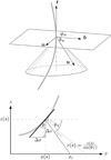Figure 1 Continuous arc-shaped source (solid grey) with accompanying Frenet trihedron (top) at the point $\mathit{x}\left(s\right) ={\left[\begin{array}{ccc}x\left(s\right)& 0& z\left(s\right)\end{array}\right]}^T,$ showing the steering angle ${\vartheta }_{\mathrm{w}}$ and inclination ϑ; see Sections 2.2–2.4 for total inclination ${\vartheta }_{\mathrm{T}}$ and the stationary-phase cone for ${\vartheta }_{\mathrm{w}}$ containing the direction u of the polar angle φw (bottom: side view).

Moreover, w shall integrate the sine of a local delay-and-sum steering angle ${\vartheta }_{\mathrm{w}}$ measured down from the normal plane of t, hence with negative sign, cf. Figure 1,

$$w=-{\int }_0^s\sin {\vartheta }_{\mathrm{w}} \mathrm{d}s.$$(4)

The Frenet–Serret formulas describe $\dot{\mathit{x}}$ as tangential vector $\mathit{t}=\dot{\mathit{x}}$, and $\ddot{\mathit{x}}=\kappa \mathit{n}$ as normal vector n scaled by curvature $\kappa = \dot{\vartheta }$, in our case $\mathit{n}={\left[\begin{array}{ccc}\cos \vartheta & 0& -\sin \vartheta \end{array}\right]}^T,$ and a bi-orthogonal vector $\mathit{b}=\mathit{t}\times \mathit{n}={\left[\begin{array}{ccc}0& 1& 0\end{array}\right]}^T$, so that ||t|| = ||n|| = ||b|| = 1 and t ⊥ n ⊥ b, cf. equation (2) and Figure 1.

2.2 Stationary-phase approximation

At high frequencies, the integrand of equation (1) oscillates rapidly. Therefore stationary phase approximation is appropriate, which evaluates the integrand’s stationary-phase points $\dot{r}+\dot{w}=0$; with derivatives abbreviated as $\frac{\mathrm{d}a}{\mathrm{d}s}=\dot{a}$, $\frac{{\mathrm{d}}^{2}a}{\mathrm{d}{s}^2}=\ddot{a}$. In typical designs, there should only be a single stationary-phase point of minimum delay $(r+w)/c$ to the receiver and therefore the pressure is approximated by,

$$p\approx \frac{e^{-\mathrm{ik}(r+w)-i\frac{\pi }{4}}}{\sqrt{8\pi k}}\frac{1}{\sqrt{r^2(\ddot{r}+\ddot{w})}}, \hspace{1em}\hspace{1em}\mathrm{at}\hspace{1em}\dot{r}=-\dot{w}.$$(5)

2.3 Target coverage

Our goal is to find the curvature and delay length w at each position s on the source such that the sound pressure

$$\left|p\right|\propto r^{-\beta }$$(6)

decays by −6β dB per doubling of distance on the listening plane that lies at z_r = 0. For an equalized magnitude square, we allow a gain g and desire

$$8\pi k{\left|p\right|}^2=\frac{1}{r^2(\ddot{r}+\ddot{w})}={\left(\frac{g}{r^{\beta }}\right)}^2 , \hspace{1em}\hspace{1em}\mathrm{at} \dot{r} = -\dot{w} .$$(7)

2.4 Stationary-phase direction

We derive $\frac{r^2}{2}$ with regard to s to describe stationary-phase directions $\dot{r} = -\dot{w}$ pointing from the corresponding point on the array emitting the first wave front received to the receiver on the listening plane at z_r = 0,

$$\frac{\mathrm{d}{r}^2}{2\mathrm{d}s}=r\dot{r}={(\mathit{x}-{\mathit{x}}_{\mathrm{r}})}^T\dot{\mathit{x}}, \hspace{1em}\Rightarrow \dot{r}=\frac{{(\mathit{x} - {\mathit{x}}_{\mathrm{r}})}^T}{r}\mathit{t}.$$(8)

We use $\dot{w}=-\sin {\vartheta }_{\mathrm{w}}$, introduce a unit-length vector $\mathit{u}=-\frac{\mathit{x}-{\mathit{x}}_{\mathrm{r}}}{r}$ to stationary-phase receivers ${\mathit{x}}_{\mathrm{r}}=\mathit{x}+r\mathit{u}$ requiring $-\dot{r}=\dot{w}$, so ${\mathit{u}}^T\mathit{t}=-\sin {\vartheta }_{\mathrm{w}}$, and these stationary-phase receivers lie on a cone of local stationary-phase directions, cf. Figure 1,

$$\mathit{u}=-\mathit{t} \sin {\vartheta }_{\mathrm{w}}+\mathit{n} \cos {\vartheta }_{\mathrm{w}} \cos {\phi }_{\mathrm{w}}+\mathit{b} \cos {\vartheta }_{\mathrm{w}} \sin {\phi }_{\mathrm{w}}=\left[\begin{array}{c}-\sin \vartheta \sin {\vartheta }_{\mathrm{w}}+\cos \vartheta \cos {\vartheta }_{\mathrm{w}} \cos {\phi }_{\mathrm{w}}\\ \cos {\vartheta }_{\mathrm{w}} \sin {\phi }_{\mathrm{w}}\\ -\cos \vartheta \sin {\vartheta }_{\mathrm{w}}-\sin \vartheta \cos {\vartheta }_{\mathrm{w}} \cos {\phi }_{\mathrm{w}}\end{array}\right].$$(9)

Below, we design the x-axis sound pressure contour at y_r = 0 for receivers at z_r = 0, simplifying the direction u with φ_w = 0 to

$$\mathit{u}{|}_{{\phi }_{\mathrm{w}}=0}=\left[\begin{array}{c}\cos (\vartheta +{\vartheta }_{\mathrm{w}})\\ 0\\ \sin (\vartheta +{\vartheta }_{\mathrm{w}})\end{array}\right],$$(10)

where the total inclination is gathered as ${\vartheta }_{\mathrm{T}}=\vartheta +{\vartheta }_{\mathrm{w}}$.

2.5 Stationary-phase magnitude

We derive $\frac{r^2}{2}$ once more from equation (8) to describe $r\ddot{r}$,

$$\frac{\mathrm{d}}{\mathrm{d}s}\left(\frac{{\mathrm{d}r}^2}{2\mathrm{d}s}\right)={\dot{r}}^2+r\ddot{r}={\dot{\mathit{x}}}^T\dot{\mathit{x}} + {(\mathit{x}-{\mathit{x}}_{\mathit{r}})}^T\ddot{\mathit{x}},$$(11)

and with ${\dot{r}}^2={\dot{w}}^2={\sin }^2 {\vartheta }_{\mathrm{w}}$, ${\sin }^2 {\vartheta }_{\mathrm{w}}=1-{\cos }^2 {\vartheta }_{\mathrm{w}}$, $\dot{\mathit{x}} = \mathit{t}$, ||t|| = 1, $\mathit{x}-{\mathit{x}}_{\mathrm{r}}=-r\mathit{u}$, $\ddot{\mathit{x}}=\dot{\vartheta }\mathit{n}$, $\mathit{t}\perp \mathit{n}\perp \mathit{b}$, as well as $\ddot{w}=-{\dot{\vartheta }}_{\mathrm{w}} \cos {\vartheta }_{\mathrm{w}}$, we get a part of ${\left|p\right|}^2$ in equation (7)

$$r\left(\ddot{r}+\ddot{w}\right)={\parallel \mathit{t}\parallel }^2 -{\dot{r}}^2+r\dot{\vartheta } {\mathit{u}}^T\mathit{n}+r \ddot{w}=1-\left[1-{\cos }^2 {\vartheta }_{\mathrm{w}}\right]-r\dot{\vartheta } \cos {\vartheta }_{\mathrm{w}} \cos {\phi }_{\mathrm{w}}-r{\dot{\vartheta }}_{\mathrm{w}} \cos { \vartheta }_{\mathrm{w}},$$(12)

and hereby the equalized magnitude squared

$$8\pi k{\left|p\right|}^2=\frac{1}{r^2}\frac{1}{\frac{{\cos }^2 {\vartheta }_{\mathrm{w}}}{r}-(\dot{\vartheta } \cos {\phi }_{\mathrm{w}}+{\dot{\vartheta }}_{\mathrm{w}}) \cos {\vartheta }_{\mathrm{w}}}.$$(13)

We assume receivers at z = 0, so ${\left[\begin{array}{ccc}0& 0& 1\end{array}\right]}^T\left[\mathit{x}+r\mathit{u}\right]=0$ retrieves r by the contributions of t, n to z in equation (9)

$$r=\frac{z}{\cos \vartheta \sin {\vartheta }_{\mathrm{w}}+\sin \vartheta \cos {\vartheta }_{\mathrm{w}} \cos {\phi }_{\mathrm{w}}}.$$(14)

2.6 Optimum total curving

To design the sound pressure response at y_r = 0, we choose φ_w = 0, yielding with ${\vartheta }_{\mathrm{T}}=\vartheta +{\vartheta }_{\mathrm{w}}$

$$\begin{array}{c}8\pi k{\left|p\right|}^2=\frac{1}{r {\cos }^2 {\vartheta }_{\mathrm{w}}-r^2{\dot{\vartheta }}_{\mathrm{T}} \cos {\vartheta }_{\mathrm{w}}}=\frac{g^2}{r^{2\beta }},\\ \mathrm{with} r=\frac{z}{\sin {\vartheta }_{\mathrm{T}}}. \end{array}$$(15)

For the current positions z, total angle ${\vartheta }_{\mathrm{T}}$, distance r from equation (15), the required angular curvature complies with the constraint equation (7) when it becomes

$${\dot{\vartheta }}_{\mathrm{T}}=-\frac{r^{2\beta }}{g^2}\frac{1}{r^2 \cos {\vartheta }_{\mathrm{w}}}+\frac{\cos {\vartheta }_{\mathrm{w}}}{r}.$$(16)

Its numerical integration using a phase/geometry split b, gain g², and start inclination ${\vartheta }_{\mathrm{offs}}$ defines Algorithm 1, where S denotes the source length and N is the number of discrete elements. The total inclination ${\vartheta }_{\mathrm{T}}$ is split into geometry and delay parts by the factors a, b, linearly, and a constant inclination offset ${\vartheta }_{\mathrm{offs}}$ is additionally added to adjust the inclination for a straight line-source with phasing only. Geometry and phase inclination parts become

$$\vartheta =a\left({\vartheta }_{\mathrm{T}}-{\vartheta }_{\mathrm{offs}}\right)+{\vartheta }_{\mathrm{offs}}, \hspace{1em}{ \vartheta }_{\mathrm{w}}=b \left({\vartheta }_{\mathrm{T}}-{\vartheta }_{\mathrm{offs}}\right)\hspace{1em}\mathrm{with} a+b=1.$$(17)

2.7 Top inclination, gain, curving split

The aiming to the audience area typically lies within $0\le {\vartheta }_{\mathrm{T}}\le \frac{\pi }{2}$ and reduces from a most horizontal aiming $\frac{\pi }{2}$ thinkable to a most upwards aiming 0 thinkable. For this reason, the total inclination decreases ${\dot{\vartheta }}_{\mathrm{T}}\le 0$ and clarifies the negative sign of ${\dot{\vartheta }}_{\mathrm{T}}$. We recognize in equation (15) that ${\dot{\vartheta }}_{\mathrm{T},0}=0$ yields the loudest sound pressure

$$g^2=\frac{r_0^{2 \beta -1}}{{\cos }^2\left({\vartheta }_{\mathrm{w},0}\right)}.$$(18)

Algorithm 1. Curving of geometry and/or phase

  procedure CURVING(x_r,0, z₀, b, β, S, N, [g², ${\vartheta }_{\mathrm{offs}}$])

    constant:

     Δs = −S/N

     ${\vartheta }_{\mathrm{T},0}$ = f(x_r,0, z₀)   ▷ according to eq. (19)

     a = 1 − b    ▷ to ensure a + b = 1

     $r_0=\sqrt{x_{\mathrm{r},0}^2+z_0^2}$    ▷ cf. Figure 2

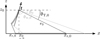Figure 2 Uniform starting conditions for both curved and phased sources: top end at x0 = 0 at s = 0, inclined by ${\vartheta }_0$, supplying the most distant listening position at xr,0, with the starting value ${\vartheta }_{\mathrm{T},0}={\vartheta }_0+{\vartheta }_{\mathrm{w},0}$. The lower end should lie at a length s = −S and supply the closest listeners at xr,S. To start at the top point, it is useful to work with a reversed integration direction −ds.

     $[{\vartheta }_{\mathrm{offs}}={\vartheta }_{\mathrm{T},0}]$    ▷ default inclination offset

     $\left[g^2=\frac{r_0^{2\beta -1}}{{\cos }^2\left[b\right({\vartheta }_{\mathrm{T},0}-{\vartheta }_{\mathrm{offs}})}\right]$    ▷ default eq. (18)

    initialization:

     w = zeros(1,N)

     x = zeros(1,N)

     z = zeros(1,N)

     r = r₀, ${\vartheta }_{\mathrm{T}}={\vartheta }_{\mathrm{T},0}$, z[1] = z₀

    for n = 1...N − 1 do

     $\vartheta =a({\vartheta }_T-{\vartheta }_{\mathrm{offs}})+{\vartheta }_{\mathrm{offs}}$    ▷ cf. eq. (17)

     ${\vartheta }_w=b({\vartheta }_T-{\vartheta }_{\mathrm{offs}})$    ▷ cf. eq. (17)

     x[n + 1] ← x[n] + $\sin \left(\vartheta \right)$ Δs    ▷ num.int. (2)

     z[n + 1] ← z[n] + $\cos \left(\vartheta \right)$ Δs    ▷ num.int. (2)

     w[n + 1] ← w[n] − $\sin \left({\vartheta }_{\mathrm{w}}\right)$ Δs    ▷ num.int. (4)

     $r\leftarrow \frac{z\left[n\right]}{\sin {\vartheta }_{\mathrm{T}}}$    ▷ according to eq. (15)

     ${\dot{\vartheta }}_{\mathrm{T}}\leftarrow f(r, {\vartheta }_{\mathrm{w}}, g^2, \beta )$    ▷ according to eq. (16)

     ${\vartheta }_{\mathrm{T}}\leftarrow {\vartheta }_{\mathrm{T}} + {\dot{\vartheta }}_{\mathrm{T}} \Delta s$    ▷ numerical integration

    end for

    return w, x, z

  end procedure

We need to ensure that the curvature ${\dot{\vartheta }}_{\mathrm{T}}<0$ stays negative yielding a convex contour and a single stationary-phase point for each observing point as implied in equation (5). Moreover, a geometrically concave solution with $\dot{\vartheta }>0$ would be impractical for line-source arrays whose splay angles $\alpha =-\dot{\vartheta } \mathrm{STEP}$ are non-negative. Choosing as a consequence both ${\dot{\vartheta }}_{\mathrm{T},0}=0$ and ${\dot{\vartheta }}_0=0$ at the top of the source, the beam-steering curvature ${\dot{\vartheta }}_{\mathrm{w},0}=0$ must also vanish to preserve ${\dot{\vartheta }}_{\mathrm{T}}=\dot{\vartheta }+{\dot{\vartheta }}_{\mathrm{w}}$.

This total inclination ${\vartheta }_{\mathrm{T},0}$ at the top of the source at x = x₀ = 0 and z = z₀ should be adjusted to ensure the top is the minimum-distance point supplying the remotest position x_r,0 in the audience as in Figure 2,

$${\vartheta }_{\mathrm{T},0}=\arctan \left(\frac{z_0}{x_{\mathrm{r},0}}\right).$$(19)

The top inclination is suggested to be purely geometrical ${\vartheta }_{\mathrm{T},0}={\vartheta }_{\mathrm{offs}}$ per default, so that its beam steering is neutral and broadside ${\vartheta }_{\mathrm{w},0}=0$ for any choice of a, b.

The simplest choices for a, and b are: (i) a = 1, b = 0 for a line source without phasing ${\vartheta }_{\mathrm{w}}\equiv 0$ but with curving $\dot{\vartheta }\ne 0$, or (ii) a = 0, b = 1 for a straight-line source without curving $\dot{\vartheta } \equiv 0$ but with phasing ${\dot{\vartheta }}_{\mathrm{w}}\ne 0$. We will also demonstrate the usefulness of mixtures in a later section, targeting the case in which multiple criteria for β should be fulfilled. For instance, the control of the curved array with equal signals fulfills the criterion β₁ = 0, and ${\beta }_2=\frac{1}{2}$ can be accomplished by additional delays.

3 Simulation studies

In this section, the differential equation will be solved numerically as outlined in Algorithm 1. It applies stepwise updates to ${\vartheta }_{\mathrm{T}}$ based on ${\dot{\vartheta }}_{\mathrm{T}}$ from equation (16). The algorithm’s step size Δs should be appropriately small to solve the problem accurately, by choosing a large N. In default of the optional argument g, Algorithm 1 uses equation (18) to define g².

The simulations below show the result of summing individual point sources described by Green’s function positioned along the continuous source contour at 1 mm intervals. This summation is performed for frequencies ranging from 20 Hz to 20 kHz with a linear resolution of 248 points, to which and a third-octave band averaging was applied. To show broadband sound pressure curves over the listening area, results were A-weighted [32] and summarized. In addition to the A-weighted on-axis sound pressure curves, a level map of a phased line source with β = 0 demonstrates the coverage including off-axis listening positions, below. Furthermore the directivity factor is discussed, calculated as result of theoretically simplified considerations, and simulated by (delayed) point sources positioned along the desired contour.

3.1 Curved line source

For curved line sources without phasing (${\vartheta }_{\mathrm{w}}\equiv 0$), a = 1 and b = 0, the design equation (15) simplifies to

$$8\pi k{\left|p\right|}^2=\frac{1}{r}\frac{1}{1-r\dot{\vartheta }}={\left(\frac{g}{r^{\beta }}\right)}^2,$$(20)

and the differential equation (16) to

$$\dot{\vartheta }=-\frac{r^{2\beta -2}}{g^2}+\frac{1}{r}\hspace{1em}\hspace{1em}\mathrm{with} r=\frac{z}{\sin \vartheta }.$$(21)

3.1.1 Comparison to literature

In a recent paper [28], we presented a second-order differential equation for β = 0, yielding an optimally curved arc source. While its result is perfectly equivalent for β = 0, the main difference lies in the formulation of the integration with regard to the x axis instead of the natural parameter s, which complicates generalization to β > 0 or comparison to literature. Equation (20) is shown above as it matches the classic equation obtained by Urban et al. [3], which states after re-writing the variables STEP = Δs, $\alpha =-\Delta \vartheta$, d = r, with $I\approx \frac{1}{\rho c}{\left|p\right|}^2$,

$$I\propto \frac{1}{r}\frac{1}{1-r\frac{\Delta \vartheta }{\Delta s}}.$$(22)

Remarkably, equation (22) resulting from a binary Fresnel-zone-based approach only differs from stationary-phase approximation equation (20) by the missing limit Δs → 0.

A later publication [5] and variable-curvature line-source tutorials [33] chose to show a simplified relation

$$I\propto -\frac{1}{r^2\frac{\Delta \vartheta }{\Delta s}},$$(23)

which is instructive and intuitively accessible. By letting $I\propto \frac{1}{g^2{r}^{2\beta }}$ and replacing $\frac{\Delta \vartheta }{\Delta s}\approx \dot{\vartheta }$, it implies

$$\dot{\vartheta }\approx -r^{2\beta -2 }{g}^{-2},$$(24)

and hereby yields the expression

$$r^{2-2\beta }\alpha \approx \mathrm{const}.$$(25)

The equation demands for cabinets pointing at large distances that the splay angle between them must be small so that more cabinets radiate into the same direction. The exponent β defines the desired distance decay. Despite its easier accessibility, however, equation (25) is inaccurate compared to equation (22) whenever β → 0 gets small. While for β = 0.5 and small Δs, it makes no substantial difference which formula is used for calculation, because either $1-r \frac{\Delta \vartheta }{\Delta s}=\mathrm{c}\mathrm{onst}.$ or $r \frac{\Delta \vartheta }{\Delta s}=\mathrm{c}\mathrm{onst}.$ approximate $I\propto \frac{1}{r}$, only with a different overall gain.

Without simplification, the equation (22) as defined in [3] yields upon targeting $I\propto \frac{1}{g^2{r}^{2\beta }}$ an approximation

$$\frac{\alpha }{\mathrm{STEP}}=g^2{r}^{2\beta -2}-\frac{1}{r}$$(26)

of equation (21), as long as STEP = Δs stays sufficiently small. In particular, the original paper used the cabinet height for STEP and the splay angles for $\alpha =-\Delta \vartheta$, i.e. a fixed geometric discretization determined by the hardware elements, as opposed to keeping it a free parameter adjusted for fine-enough discretization Δs → 0, when numerically solving a differential equation.

3.1.2 Curved line source: results

The differential equation of equation (21) is solved numerically by the proposed Algorithm 1 with uniform parameters x_r,0 = 10 m, z₀ = 2.072 m, b = 0 and source length S = 1.312 m for all decays, giving the number of discrete elements N = 1313 for a step size Δs = 1 mm. Equation (19) specifies the total inclination on top of the source ${\vartheta }_{\mathrm{T},0}=11.31\mathrm{°}$ and for β = 0, the gain parameter is calculated by equation (18) yielding a value of $g= \frac{1}{\sqrt{10.2124}}$. For the other decay values, g was set manually to g = 0.443 for β = 0.25 and g = 0.599 for β = 0.5, in order to supply the same listening positions 0 ≤ x_r ≤ 10 m with unchanged source length S.

Figure 3 shows the source contour for different decays and Figure 4 the resulting A-weighted sound pressure profiles with dB offsets to make the β = {0, 0.25, 0.5} curves to go through {0, −3.5, −7} dB at the distance of x_r = 4 m. The levels do not follow the theoretical roll-off curves −6β dB per doubling of the distance beyond x_r > 7 m as stationary phase approximation assumes an infinite line integral although the actual length is finite.

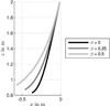Figure 3 Curved line source contours for different decays β.

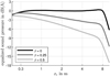Figure 4 A-weighted sound pressure levels of curved line sources for different decays β with mixed x-axis scaling, linear for xr ≤ 1 and logarithmic for xr > 1, with the target range 0 ≤ xr ≤ 10 m.

Another parameter to be considered for radiation characteristics is the directivity factor Q. Figure 5 shows the directivity index DI = 10 lg Q for both cases, curved and phased line source with different decays β. The radiation of the source was calculated at 10 m distance as summation of individual point sources with Δs = 1 mm. For low frequencies, omnidirectional radiation is seen, which coincides with theoretical considerations for frequencies below 130 Hz ($\frac{\lambda }{2}$). At frequencies above 500 Hz, the curves for different decay values differ, with small decay values leading to higher directivity. With $a\approx \frac{r_0}{r_{\mathrm{S}}},$ Sections A.3 and A.4 we find

$$\mathrm{DI} \approx \{\begin{array}{c}10\lg \left(1+\frac{k\mathrm{S}}{\pi }\right),\hspace{1em}\hspace{1em}\&\hspace{1em}\hspace{1em}\mathrm{for}\hspace{1em}f<\frac{c}{2∆x},\\ 3+10\lg \frac{a}{\ln a},\hspace{1em}\hspace{1em}\&\hspace{1em}\hspace{1em}f\to \mathrm{\infty }\hspace{1em}\mathrm{for} \beta =\frac{1}{2},\\ 3+10\lg \frac{a}{1-a^{-1+2\beta }}, \&\hspace{1em}\hspace{1em}f\to \mathrm{\infty }\hspace{1em}\mathrm{for} \beta \ne \frac{1}{2}.\end{array}$$(27)

The results are shown as dotted lines in Figure 5 and show the same trends as the simulated solid lines, where a = 7 corresponds to the ratio of distances, within which the level curves fulfill the decay profile, cf. Figure 4. The horizontal extent Δx is 9.83 cm for β = 0, it is 19.82 cm for β = 0.25, and 32.14 cm for β = 0.5.

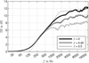Figure 5 Directivity index for curved (thin) and phased (bold) line sources with different decays β compared to equation (27) (dotted).

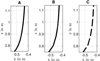Figure 6 Discretization of a continuously curved line source (A) according to the β = 0 example from Figure 3 to: a polygon of straight-line sources with splay angles rounded to integer degrees (B) and gaps between these straight-line segments (C); graphs are rotated by ${\vartheta }_{\mathrm{offs}}$ and limited to z < 1.15 m for easy readability.

Professional line-source array systems typically contain multi-way transducers, of which the larger layout of the low- and mid-frequency transducers is horizontally directional, instead of radiating axisymmetrically. Similarly, their vertical high frequency line-source transducers, e.g. f > 1 kHz, are typically equipped with horizontal waveguides or wedge-shaped horns that limit horizontal radiation to 110°, so roughly a third of the 360° panorama, or to 70° which is roughly its fifth. The modeled DI can be adapted correspondingly with an increase by +5 dB for 110° or +7 dB for 70° horizontal coverage.

3.1.3 Discretization of source and splay angles

Later we will use a prototype of a line array to show the effectiveness of the formalism in practice. Since is solved with the same parameters as in Section 3.1.2 and the resulting continuous source is then composed by point sources that are positioned along the contour, cf. Figure 7A. To simulate a practical device built from discrete elements, the contour was discretized into a polygon of 8.2 cm straight-line segments in Figure 7B. The splay angles are chosen so that the error made in the total inclination caused by using integer ° values for the splay angles is kept minimal. The same procedure is executed for Figure 7C but with shorter 6.2 cm straight-line segments with the same splay angles but leaving gaps in between. Due to discretization with integer-degrees splay angles, the lost control of small curvatures yields a boost of the sound pressure level between 7 m and 8 m for β = 0 in our example, cf. Figure 7. Gaps between the straight-line source elements weaken the attenuation of spatial aliasing. It occurs at frequencies above $f>\frac{c}{0.082}\approx 4.2 \mathrm{kHz}$ where the inter-element spacing exceed a wavelength, which causes a noticeable downwards leakage of sound to listeners at x_r < 3 m with broadside steering ${\vartheta }_{\mathrm{w}}=0$.

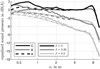Figure 7 A-weighted sound pressure level for different decays β and different discretization with mixed x-axis scaling, linear for xr ≤ 1 and logarithmic for xr > 1, as above; continuous line source (dotted), discrete point sources with 8.2 cm (dashed), straight 6.2 cm line-sources at the same spacing with inclination increments rounded to integer ° values (solid).

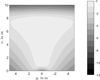Figure 8 Simulated A weighted sound pressure map of a phased line source for β = 0 over a listening area of 10 m × 10 m.

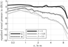Figure 9 A-weighted sound pressure levels of a phased source with different decays β for a target range 0 ≤ xr ≤ 10 m, with a continuous source Figure 6A or discrete segments Figure 6C of integer sample delays (48 kHz sample rate); the x-axis is scaled linearly for xr ≤ 1 and logarithmically for xr > 1.

3.2 Phased straight-line source

With a = 0, we get the differential equation for the beamforming angle of a straight-line source from equation (16),

$${\dot{\vartheta }}_{\mathrm{w}}=-\frac{r^{2\beta -2}}{g^2 \cos {\vartheta }_{\mathrm{w}}}+\frac{\cos {\vartheta }_{\mathrm{w}}}{r}\hspace{1em}\hspace{1em}\mathrm{with}\hspace{1em}r=\frac{z}{\sin {\vartheta }_{\mathrm{T}}}.$$(28)

3.2.1 Phased straight-line source: results

The differential equation (28) is solved numerically by Algorithm 1 with uniform parameters x_r,0 = 10 m, z₀ = 2.117 m, b = 1, ${\vartheta }_{\mathrm{w},0}=0$ and source length S = 1.312 m for all decay values, resulting in the number of discrete elements N = 1313 for a step size Δs = 1 mm. Equation (19) defines the inclination on top of the source ${\vartheta }_{\mathrm{T},0}={\vartheta }_{\mathrm{offs}}=11.365$° and for β = 0, the gain parameter is calculated by equation (18) yielding a value of $g=\frac{1}{\sqrt{10.2124}}$. For the other decay values, g was set manually, g = 0.449 for β = 0.25 and g = 0.614 for β = 0.5. Figure 10 shows the delay lengths for different decay values, and Figure 9 describes the resulting A-weighted sound pressure curves for a continuously phased source (dotted lines) compared to direct sound pressures curves of a discrete phased source with enclosure height 8.2 cm, gaps in between and rounded delays being accurate to 1 sample at f_s = 48 kHz. The SPL plots for the continuous source exhibit the same trend as those for the purely curved source. For very close listening positions, the curves differ due to discretization and spatial aliasing. The delays also cause a comb filter, which is greatest at β = 0 due to the temporal structure of the summed impulse response and has the opposite effect to spatial aliasing. The A-weighted sound pressure for β = 0 including off-axis listening positions can be found as a level map in Figure 8 over a 10 m × 10 m listening area. The coverage for which level changes stays below 1 dB reaches a limit of |φ_w| = 27.5° for closer observation points. For farther observation points (5 m < x_r < 7.8 m) the coverage gets wider up to maximum of |φ_w| = 35° for r = 8.5 m.

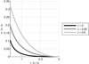Figure 10 Delay length w for different decays β.

3.2.2 Comparison to literature

Electronically steered line arrays for sound reinforcement can be found in literature, however not fixed to using delays, only. Meyer [14, 34] employs individual filters to control each array loudspeaker and proposes to mount the line arrays along the ceiling. Different designs are used with regard to the arrays’ throw distance, short-throw vs. long-throw array, and to keep the direct sound coverage of the audience flat. Van der Werff [15] discusses wall-mounted line arrays with non-uniformly spaced transducers, as nested array, with individual filtering with IIR low-pass filter designs. The goal of his work is to increase the direct-to-reverberant ratio in large halls by achieving a flat direct sound pressure level profile of 0 dB per distance doubling, and the design was verified in EASE 1.2. And finally, Duran Audio’s Digital Directivity Synthesis is a well-known DSP-assisted method based on least-squares for uniformly spaced line arrays [11]. Its optimization of the desired direct sound pressure level profiles takes transducer directivity into account. The method requires the implementation of FIR filters as signal processing done for each loudspeaker.

Algorithm 2. Two-target curving of geometry and phase

  procedure TWOBETA(x_r,0, z₀, β₁, β₂, S, N, $g_1^2,g_2^2$, ${\vartheta }_{\mathrm{offs}}$)

    constant:

     Δs = −S/N

     ${\vartheta }_0$ = f(x_r,0, z₀)    ▷ according to eq. (19)

     $r_0=\sqrt{x_{r,0}^2+z_0^2}$    ▷ cf. Figure 2

    initialization:

     w = zeros(1,N)

     x = zeros(1,N)

     z = zeros(1,N)

     r₁ = r₂ = r₀, $\vartheta \left[1\right]={\vartheta }_0$, z[1] = z₀

    for n = 1...N − 1 do

     w[n + 1] ← w[n] − $\sin \left({\vartheta }_{\mathrm{w}}\right)$ Δs    ▷ num.int. (4)

     x[n + 1] ← x[n] + $\sin \left(\vartheta \right)$ Δs    ▷ num.int. (2)

     z[n + 1] ← z[n] + $\cos \left(\vartheta \right)$ Δs    ▷ num.int. (2)

     $r_1\leftarrow \frac{z\left[n\right]}{\sin \vartheta }, \hspace{1em}{r}_2\leftarrow \frac{z\left[n\right]}{\sin (\vartheta +{\vartheta }_{\mathrm{w}})}$    ▷ cf. eq. (15)

     $\dot{\vartheta }\leftarrow f(r_1, g_1^2, {\beta }_1)$    ▷ according to eq. (21)

     $\vartheta \leftarrow \vartheta +\dot{\vartheta } \Delta s$    ▷ numerical integration

     ${\dot{\vartheta }}_{\mathrm{w}}\leftarrow f(r_2, {\vartheta }_{\mathrm{w}}, \dot{\vartheta }, g_2^2, {\beta }_2)$    ▷ acc. to eq. (29)

     ${\vartheta }_{\mathrm{w}}\leftarrow {\vartheta }_{\mathrm{w}}+ {\dot{\vartheta }}_{\mathrm{w}} \Delta s$    ▷ numerical integration

    end for

    return w, x, z

  end procedure

3.3 Curved and phased line source

To support two simultaneous coverage designs (preserving mixing-balance and envelopment) for a large audience area, phasing delays are used in combination with geometrical curving. In addition to a decay β₁ accomplished by driving the cabinets of a curved array with identical signals, delays between individually driven cabinets can be used to satisfy an alternative decay β₂.

First, equation (21) is solved for a purely curved source (b = 0) with β₁ as shown in Algorithm 1, and afterwards the required delay lengths for another choice of β₂ is calculated preserving the geometrical curvature $\dot{\vartheta }$,

$${\dot{\vartheta }}_{\mathrm{w}}=-\frac{r^{2{\beta }_2}}{g^2}\frac{1}{r^2\cos {\vartheta }_{\mathrm{w}}}+\frac{\cos {\vartheta }_{\mathrm{w}}}{r}-\dot{\vartheta },$$(29)

which is summarized in Algorithm 2.

As this design and algorithm will be analyzed in measurements using prototypical hardware in the next section, graphical analysis of the results will be shown below.

4 Experimental setup

To show the effectiveness of the formalism in practice, the reproducible miniature line array presented in [35] was used, cf. Figure 11. The trapezoidal shape was chosen so that a maximum tilt angle of 10 degrees can be set. SB Acoustics SB65WBAC25-4 were used as the 2.5-inch full-range speakers.

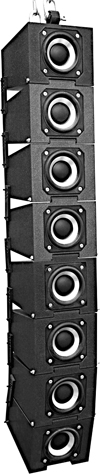Figure 11 Miniature Line Array of eight 3D printed enclosures (closed 0.4 l boxes).

For the measurements, 12 enclosures are lined up for which we obtain the continuous source contour and delay lengths from Algorithm 1. The measurements took place in an auditorium (30 m × 9 m × 3.5 m) with a reverberation time of T₆₀ ≈ 0.82 s. To focus on verifying the direct sound design, the impulse responses were truncated to the first 300 samples (6.25 ms at f_s = 48 kHz). The gain values g for β = 0 are calculated by equation (18), for the other decay values g was set manually, g = 0.46 for β = 0.25 and g = 0.65 for β = 0.5. The solution is then discretized using a step size of 8.2 cm which corresponds to the distance between two neighbouring drivers. In order to record the position-dependent direct sound pressure level curves, impulse responses were measured along 20 positions (on-axis) starting at x_r = 1 m and ending at x_r = 10.5 m. Pressure zone microphones were positioned on the ground to avoid floor reflections in the measurements. We applied equalization to obtain a flat frequency response between 200 Hz and 20 kHz for the single array element. Moreover, a filter with magnitude increasing by $\sqrt{f}$ until the spatial aliasing frequency was employed to equalize the otherwise pink sound pressure of a linear arrangement of ideal point sources, cf. equation (7). The results are averaged in third octaves and the curves are plotted as A-weighted sum.

4.1 Curved line source

Figure 12 shows the A weighted sum over distance (on-axis) for different decays β compared to the simulated curves with the same discretization as in Figure 6C. The measured results show almost identical curves to the simulation and the artefacts caused by discretization of source and splay angles are observed.

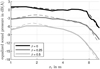Figure 12 A-weighted measured sound pressure of curved arrays (solid) with different decays over distance compared to the simulated discretized source (dashed) with rounded splay angles keeping the error made in total inclination minimal.

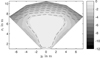Figure 13 Measured A weighted sound pressure map of a phased array with β = 0 compared to simulated contours in steps of 1 dB (dashed).

4.2 Phased line source

Figure 14 shows the A-weighted on-axis sound pressure curves in comparison to the simulated for different decays β. Also here, the measured results follow almost the theoretical simulated based on point source summation. The noticeable differences are close to the source where the beamforming no longer reaches closer listening positions and spatial aliasing affects the results. Figure 13 presents the measured coverage (solid) including off-axis listening positions of a phased array with β = 0 compared to the simulated (dashed). We observe a lower sound pressure for lateral listening positions because the linearly arranged point sources in the simulation do not take the horizontal directivity of the drivers into account.

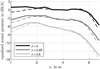Figure 14 A-weighted measured sound pressure of phased arrays (solid) with different decays over distance compared to the simulated discretized source (dashed) with rounded delays at fs = 48 kHz.

4.3 Mixed curve and phase design

For the mixed design, we take the curved line source from Section 4.1 with β₁ = 0 and use the corresponding time of flight to satisfy β₂ = 0.5 according to Algorithm 2. The rounded delays at f_s = 48 kHz were inserted in the off-line analysis. Figure 15 shows the A-weighted sound pressure profile of a purely curved source with β = 0 and compares the A-weighted profile of a curved line source with β = 0.5 with the curve of the mixed design.

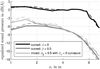Figure 15 A-weighted measured sound pressure of curved arrays (solid) with decays β = 0 and β = 0.5 and mixed array with β1 = 0 and β2 = 0.5 over distance compared to simulated discretized sources (dashed).

The profile for a purely curved source and the one of the mixed design differ in the vicinity of the source only, because the impulse responses of the enclosures differ in time structure in this area, yielding a different sum. Nevertheless, both follow the simulated −3 dB per doubling of distance.

5 Conclusion

This paper presented design equations for continuously curved and phased line sources with the target to accomplish desired sound pressure roll-offs. The stationary phase approximation was applied to the contour integral of a Green’s function with delay (phasing) to obtain a second-order nonlinear differential equation for curving and phasing. The discretized results are directly applicable to design curvature and phasing of discrete line source arrays. Simulations of the continuous source based on summation of point sources positioned along the line source contour showed the ideal −6β dB profiles per doubling of the distance. Furthermore, the simulations revealed the effects caused by the discretization of the source. The theoretical results were underlined by measurements of a line array prototype. Moreover, the results showed that a two-target design based on curving and phasing is feasible.

Future work should consider psychoacoustic evaluations of line sources with different β profiles for medium-sized immersive sound reinforcement for 50–250 listeners to assess improvements in envelopment and direct-sound mix. Experiments should also take frequency-response homogeneity into account, which is often optimized as a trade-off with the coverage parameter β, see also [33].

Acknowledgments

Our research was funded by the Austrian Science Fund (FWF): P 35254-N, Envelopment in Immersive Sound Reinforcement (EnImSo). The authors thank Thomas Musil for his design improvements on our miniature line array.

Conflict of interests

The authors declared no conflicts of interests.

Data Availability Statement

The research data associated with this article are included in the supplementary material of this article [36].

Appendix

A.1 Line array near field

When observing a line source of the length S at the normal distance r to one of its ends, the distance to its other end is $\sqrt{r^2 +S^2}$. A distance difference $\sqrt{r^2 +S^2}-r$ to both ends that may exceed a $\frac{\pi }{2}$ phase shift towards r → 0 defines the acoustic near field, within which the distance decay can differ from $\frac{1}{r}$, with $k=\frac{2\pi f}{c}$ and $\sqrt{1 + x}\approx 1 + \frac{x}{2}$,

$$\mathrm{kr}\sqrt{1+\frac{S^2}{r^2}}-\mathrm{kr}=\frac{\pi }{2}$$

$$k\frac{S^2}{2r}\approx \frac{\pi }{2},\hspace{1em}\hspace{1em}\Rightarrow r=\frac{2f{S}^2}{c}.$$(A.1)

Example: The near field extends to 10 m for a source of the length 1 m at a frequency of f = 5c = 1.7 kHz.

A.2 Line array aliasing

A line array composed of discrete elements of the height and spacing h driven in phase radiates waves focused to directions perpendicular to the line. It exhibits uncontrolled radiation due to spatial aliasing at and above the frequency at which also waves propagating along the line fit the in-phase control,

$$\mathrm{kh}\ge 2\pi ,\hspace{1em}\hspace{1em}\Rightarrow f\ge \frac{c}{h}.$$(A.2)

Example: The frequency should stay below 3 kHz for $h=\frac{c}{3000}=11.4 \mathrm{cm}$ to avoid spatial aliasing.

A.3 Directivity index of a line source

For very low frequencies f → 0, any phased/curved line source has vanishing extent in terms of wavelengths and the directivity index is zero DI → 0 dB.

Any phased/curved line source exhibits a length S as its larger geometric extent. Its directivity index first rises when the length S exceeds half a wavelength $\frac{\lambda }{2}=\frac{1}{2}\frac{c}{f}$

$$f_1=\frac{c}{2S}.$$(A.3)

Around this frequency, the directivity function is well approximated by a line source of the length S, with $\frac{1}{S}{\int }_{-\frac{S}{2}}^{\frac{S}{2}}{e}^{\mathrm{ikz}\sin \vartheta }\mathrm{d}z=\frac{1}{S}\frac{2 \sin (k\frac{S}{2}\sin \vartheta )}{k\sin \vartheta }$. The directivity factor of an axisymmetric radiation is 2 divided by the squared directivity pattern integrated along the inclination d sin ϑ,

$$Q=\frac{2S^2}{4{\int }_0^1\frac{{\sin }^2\left(k\frac{S}{2}\sin \vartheta \right)}{k^2{\sin }^2 \vartheta }\mathrm{d} \sin \vartheta }$$(A.4)

$$=\frac{k^2{S}^2}{\mathrm{kS} \mathrm{Si}\left(k\mathrm{S}\right)+\cos \left(k\mathrm{S}\right)-1},$$(A.5)

and at low frequencies we approximate the sine integral Si(kS) by kS and cosine cos(kS) by 1, yielding Q ≈ 1, and the asymptotic value of Si(kS) is $\frac{\pi }{2}$ at high frequencies, where we may neglect cos(kS) + 1 and get $Q\approx \frac{\mathrm{kS}}{\pi }$, or in total

$$Q\approx 1+\frac{\mathrm{kS}}{\pi }.$$(A.6)

After the linear increase of the directivity factor above $\frac{\mathrm{kS}}{\pi }>1$, a slight saturation will be reached when the second extent of the curved/phased line source $\Delta x=x_{\mathrm{S}}-S \cos {\vartheta }_0$ or Δx = w_S exceeds half a wavelength

$$f_2=\frac{c}{2\Delta x}=\frac{S}{\Delta x}{f}_1,$$(A.7)

which is conveniently denoted as frequency f₁ scaled by the approximate aspect ratio $\frac{S}{\Delta x}$ of the source.

A.4 Directivity index of a directional point source with predefined coverage

To estimate the directivity index, we consider the far-field sound pressure of a directional point source,

$$p\left(r\right)=\frac{e^{-\mathrm{ikr}}}{4\pi r}g(\sin \vartheta )$$(A.8)

mounted at the height z₀ above the audience and exhibiting a roughly axisymmetric directivity function g around the vertical axis. Listeners at ear height are reached if the distance r relates to the variable inclination angle by

$$r=\frac{z_0}{\sin \vartheta },$$(A.9)

and a correspondingly re-formulated directivity factor depending on this r can be tailored so that listeners receive

$$\left|p\left(r\right)\right|={\left(\frac{r_0}{r}\right)}^{\beta }, \hspace{1em}\hspace{1em}\mathrm{with} g\left(r\right)=4\pi r{\left(\frac{r_0}{r}\right)}^{\beta },$$(A.10)

and hereby a well-controlled direct-sound level decaying with −6β dB per doubling of the distance. To avoid radiation to angles outside ${\vartheta }_{\mathrm{s}}\le \vartheta \le {\vartheta }_0$, the directivity function must vanish elsewhere, accordingly, and we may substitute $r_{\mathrm{s}}=\frac{r_0}{a}$and choose r_s = z₀ for simplicity,

$$g\left(r\right)=0, \hspace{1em}\hspace{1em}\mathrm{for} r<\frac{r_0}{a}\hspace{0.5em}\mathrm{and}\hspace{0.5em}r>r_0.$$(A.11)

The characterization of a directivity pattern relies on observation at a direction-independent distance, e.g. r₀, but we may keep r as unrelated variable defining the directivity function g by the angle-dependent distance to the listeners,

$$\left|p\right(r_0\left)\right|=\frac{g\left(r\right)}{4\pi r_0}={\left(\frac{r_0}{r}\right)}^{\beta -1}.$$(A.12)

With the directivity pattern integrated along the inclination $\cos \vartheta \mathrm{d}\vartheta =-\mathrm{d} \sin \vartheta =\frac{z_0}{r^2}\mathrm{d}r=\frac{r_0}{a}\frac{\mathrm{d}r}{r^2}$ the directivity factor of the axisymmetric radiation is

$$Q=\frac{2}{{\int }_0^{\pi }{\left|p\right|}^2\cos \vartheta \mathrm{d}\vartheta }=\frac{2a{r}_0^{1-2\beta }}{{\int }_{\frac{r_0}{a}}^{r_0}{r}^{-2\beta }\mathrm{d}r}=\{\begin{array}{c}\frac{2a(1-2\beta )}{1-a^{-1+2 \beta }},\hspace{1em}\hspace{1em} \beta \ne \frac{1}{2},\\ \frac{2a}{\ln \left(a\right)},\hspace{1em}\hspace{1em}\hspace{1em}\hspace{1em}\hspace{1em}\hspace{1em}\beta =\frac{1}{2}.\end{array}$$(A.13)

For curved/phased line-source arrays, this rough asymptotic approximation can be assumed to hold for high frequencies f > f₂, where the directivity function vanishes outside the angular range ${\vartheta }_{\mathrm{s}}\le \vartheta \le {\vartheta }_0$.

References

All Figures

Figure 1 Continuous arc-shaped source (solid grey) with accompanying Frenet trihedron (top) at the point $\mathit{x}\left(s\right) ={\left[\begin{array}{ccc}x\left(s\right)& 0& z\left(s\right)\end{array}\right]}^T,$ showing the steering angle ${\vartheta }_{\mathrm{w}}$ and inclination ϑ; see Sections 2.2–2.4 for total inclination ${\vartheta }_{\mathrm{T}}$ and the stationary-phase cone for ${\vartheta }_{\mathrm{w}}$ containing the direction u of the polar angle φw (bottom: side view).

In the text

Figure 2 Uniform starting conditions for both curved and phased sources: top end at x0 = 0 at s = 0, inclined by ${\vartheta }_0$, supplying the most distant listening position at xr,0, with the starting value ${\vartheta }_{\mathrm{T},0}={\vartheta }_0+{\vartheta }_{\mathrm{w},0}$. The lower end should lie at a length s = −S and supply the closest listeners at xr,S. To start at the top point, it is useful to work with a reversed integration direction −ds.

In the text

	Figure 3 Curved line source contours for different decays β.
In the text

	Figure 4 A-weighted sound pressure levels of curved line sources for different decays β with mixed x-axis scaling, linear for xr ≤ 1 and logarithmic for xr > 1, with the target range 0 ≤ xr ≤ 10 m.
In the text

	Figure 5 Directivity index for curved (thin) and phased (bold) line sources with different decays β compared to equation (27) (dotted).
In the text

	Figure 6 Discretization of a continuously curved line source (A) according to the β = 0 example from Figure 3 to: a polygon of straight-line sources with splay angles rounded to integer degrees (B) and gaps between these straight-line segments (C); graphs are rotated by ${\vartheta }_{\mathrm{offs}}$ and limited to z < 1.15 m for easy readability.
In the text

	Figure 7 A-weighted sound pressure level for different decays β and different discretization with mixed x-axis scaling, linear for xr ≤ 1 and logarithmic for xr > 1, as above; continuous line source (dotted), discrete point sources with 8.2 cm (dashed), straight 6.2 cm line-sources at the same spacing with inclination increments rounded to integer ° values (solid).
In the text

	Figure 8 Simulated A weighted sound pressure map of a phased line source for β = 0 over a listening area of 10 m × 10 m.
In the text

	Figure 9 A-weighted sound pressure levels of a phased source with different decays β for a target range 0 ≤ xr ≤ 10 m, with a continuous source Figure 6A or discrete segments Figure 6C of integer sample delays (48 kHz sample rate); the x-axis is scaled linearly for xr ≤ 1 and logarithmically for xr > 1.
In the text

	Figure 10 Delay length w for different decays β.
In the text

	Figure 11 Miniature Line Array of eight 3D printed enclosures (closed 0.4 l boxes).
In the text

	Figure 12 A-weighted measured sound pressure of curved arrays (solid) with different decays over distance compared to the simulated discretized source (dashed) with rounded splay angles keeping the error made in total inclination minimal.
In the text

	Figure 13 Measured A weighted sound pressure map of a phased array with β = 0 compared to simulated contours in steps of 1 dB (dashed).
In the text

	Figure 14 A-weighted measured sound pressure of phased arrays (solid) with different decays over distance compared to the simulated discretized source (dashed) with rounded delays at fs = 48 kHz.
In the text

	Figure 15 A-weighted measured sound pressure of curved arrays (solid) with decays β = 0 and β = 0.5 and mixed array with β1 = 0 and β2 = 0.5 over distance compared to simulated discretized sources (dashed).
In the text

References

- W. Ahnert, D. Noy: Sound reinforcement for audio engineers, Taylor & Francis Ltd, 2023. [Google Scholar]
- C. Heil, M. Urban, Sound fields radiated by multiple sound sources arrays, in: 92nd AES Conv, Vienna, 1992. [Google Scholar]
- M. Urban, C. Heil, P. Bauman: Wavefront sculpture technology. Journal of the Audio Engineering Society 51, 10 (2003) 912–932. [Google Scholar]
- F. Straube, F. Schultz, M. Makarski, S. Spors, S. Weinzierl: Evaluation strategies for the optimization of line source arrays, in: 59th AES Conf, Montreal, Canada, 2015. [Google Scholar]
- F. Straube, F. Schultz, D.A. Bonillo, S. Weinzierl: An analytical approach for optimizing the curving of line source arrays. Journal of the Audio Engineering Society 66, 1/2 (2018) 4–20. [CrossRef] [Google Scholar]
- A. Hölter, F. Straube, F. Schultz, S. Weinzierl: Enhanced polygonal audience line curving for line source arrays, in: 150th AES Convention, 2021. [Google Scholar]
- A. Thompson: Line array splay angle optimisation, in: Reproduced Sound 22 Conference, Oxford, 2006. [Google Scholar]
- A. Thompson, Improved methods for controlling touring loudspeaker arrays, in: 127th AES Convention, New York, USA, 2009. [Google Scholar]
- A. Thompson, J. Baird, B. Webb, Numerically optimized touring loudspeaker arrays – practical applications, in: 131st AES Convention, New York, USA, 2011. [Google Scholar]
- F. Toole, Sound Reproduction: Loudspeakers and Rooms, in: Audio Engineering Society Presents Series, Elsevier, 2008. [Google Scholar]
- G. van Beuningen, E. Start: Optimizing directivity properties of DSP controlled loudspeaker arrays, in: Reproduced Sound 16 Conference, Stratford upon Avon, 2000. [Google Scholar]
- D. Ward, R. Kennedy, R. Williamson: Constant directivity beamforming, in: Microphone Arrays, Springer, Berlin, Heidelberg, 2001, pp. 3–17. [CrossRef] [Google Scholar]
- M. Goodwin, G. Elko: Constant beamwidth beamforming, in: IEEE ICASSP, Vol. 1, Minneapolis, USA, 1993, pp. 169–172. [CrossRef] [Google Scholar]
- D.G. Meyer: Digital control of loudspeaker array directivity. Journal of the Audio Engineering Society 32, 10 (1984) 747–754. [Google Scholar]
- J. van der Werff, Design and implementation of a sound column with exceptional properties, in: 96th AES Convention, Amsterdam, Netherlands, 1994. [Google Scholar]
- R. Mailloux: Phased array antenna handbook, 3rd edn., Artech House, 2017. [Google Scholar]
- T. Taylor: Design of line-source antennas for narrow beamwidth and low side lobes. Transactions of the IRE Professional Group on Antennas and Propagation 3, 1 (1955) 16–28. [CrossRef] [Google Scholar]
- P. McManamon, T. Dorschner, D. Corkum, L. Friedman, D. Hobbs, M. Holz, S. Liberman, H. Nguyen, D. Resler, R. Sharp, E. Watson: Optical phased array technology. Proceedings of the IEEE, 84, 2 (1996) 268–298. [CrossRef] [Google Scholar]
- H. Shanks: A geometrical optics method of pattern synthesis for linear arrays. IRE Transactions on Antennas and Propagation 8, 5 (1960) 485–490. [CrossRef] [Google Scholar]
- B. Chiang, D.H.-S. Cheng: Curvilinear arrays. Radio Science 3, 5 (1968) 405–409. [CrossRef] [Google Scholar]
- A. Chakraborty, B. Das, G. Sanyal: Determination of phase functions for a desired onedimensional pattern. IEEE Transactions on Antennas and Propagation 29, 3 (1981) 502–506. [CrossRef] [Google Scholar]
- E. Start: Direct sound enhancement by wavefield synthesis. Ph.D. dissertation Technical University Delft, 1997. [Google Scholar]
- G. Firtha: A generalized wave field synthesis framework with application for moving virtual sources. Ph.D. dissertation Budapest University of Technologies and Economics, 2019. [Google Scholar]
- P. Grandjean, A. Berry, P.-A. Gauthier: Sound field reproduction by combination of circular and spherical higher-order ambisonics: part I — a new 2.5-d driving function for circular arrays. Journal of Audio Engineering Society 69, 3 (2021) 152–165. [CrossRef] [Google Scholar]
- F. Schultz: Sound field synthesis for line source array applications in large-scale sound reinforcement. Ph.D. dissertation University of Rostock, 2016. [Google Scholar]
- SMPTE RP 2096–1:2017, Recommended practice – cinema sound system baseline setup and calibration, 2017. [Google Scholar]
- J. Nettingsmeier, D. Dohrmann: Preliminary studies on large-scale higher-order ambisonic sound reinforcement systems, in: Ambisonics Symposium, Lexington, KY, 2011. [Google Scholar]
- L. Gölles, F. Zotter: Optimally curved arc source for sound reinforcement, in: Fortschritte der Akustik, DAGA, Vienna, 2021. [Google Scholar]
- F. Zotter, S. Riedel, L. Gölles, M. Frank: Acceptable imbalance of sound-object levels for off-center listeners in immersive sound reinforcement, in: Fortschritte der Akustik, DAGA, Hamburg, 2023. [Google Scholar]
- S. Riedel, F. Zotter: Surrounding line sources optimally reproduce diffuse envelopment at offcenter listening positions JASA Express Letters 2, 9 (2022) 094404. [CrossRef] [PubMed] [Google Scholar]
- S. Riedel, L. Gölles, F. Zotter, M. Frank: Modeling the listening area of envelopment, in: Fortschritte der Akustik, DAGA, Hamburg, 2023. [Google Scholar]
- ÖVE/ÖNORM EN 61672–1: Electroacoustics – Sound level meters – Part 1: Specifications, OVE/Austrian Standards Institute, Vienna, AT, Standard, 2015. [Google Scholar]
- F. Montignies: Understanding line source behaviour – for better optimization, in: VCLS Tutorial, AES, 2020. [Google Scholar]
- D.G. Meyer: Multiple-beam, electronically steered line-source arrays for sound-reinforcement applications. Journal of the Audio Engineering Society 38, 4 (1990) 237–249. [Google Scholar]
- L. Gölles, F. Zotter, L. Merkel: Miniature line array for immersive sound reinforcement, in: Proceedings of AES SIA Conf., Huddersfield, 2023. [Google Scholar]
- L. Gölles and F. Zotter: Supplementary material for theory of continuously curved and phased line sources for sound reinforcement. [Online]. Available at https://phaidra.kug.ac.at/o:129841. [Google Scholar]
Cite this article as: Gölles L. & Zotter F. 2023. Theory of continuously curved and phased line sources for sound reinforcement. Acta Acustica, 7, 52.