| Issue |
Acta Acust.
Volume 9, 2025
|
|
|---|---|---|
| Article Number | 39 | |
| Number of page(s) | 14 | |
| Section | Audio Signal Processing and Transducers | |
| DOI | https://doi.org/10.1051/aacus/2025023 | |
| Published online | 25 June 2025 | |
Scientific Article
Abnormal noise detection of electric machines based on HPSS-CIS and CNN-CBAM
1
College of Mechanical Engineering, Xi’an Jiaotong University Xi’an 710049 PR China
2
School of Mechanical and Electrical Engineering, Xi’an Polytechnic University Xi’an 710049 PR China
* Corresponding author: This email address is being protected from spambots. You need JavaScript enabled to view it.
Received:
22
November
2024
Accepted:
25
May
2025
Abstract
For a long time, the traditional motor manufacturing industry relies on the artificial hearing method to identify whether there is abnormal noise in the motor, thus leading to low efficiency and poor accuracy consistency. To solve these problems, a new prediction method based on the algorithm of harmonic percussion sound separation (HPSS) and continuous interphase sampling (CIS) of cochlear implants and the CNN-CBAM (Convolutional neural network based on Convolutional Block Attention Module) model, is proposed in this paper. Firstly, the original sound signals are separated into harmonic and percussive components by the HPSS algorithm, and then each component is processed by the CIS algorithm of cochlear implant to obtain electrode stimulation signal that can simulate human hearing. Subsequently, the classification task of motors are achieved by a deep learning model that combines CNN and CBAM. The proposed method is verified that the highest accuracy of 99.27% is achieved in the motor data set. Afterward for feature extraction, the results of ablation experiments with HPSS-CIS show that the average accuracy of this method is more than 4.5% higher than that of any single component. In addition, for the human auditory feature extraction method after HPSS processing, the CIS method is compared with the widely used Mel filter bank, and shows better performance.
Key words: Harmonic percussion sound separation / Continuous interphase sampling / Convolutional block attention module / Abnormal noise detection
© The Author(s), Published by EDP Sciences, 2025
 This is an Open Access article distributed under the terms of the Creative Commons Attribution License (https://creativecommons.org/licenses/by/4.0), which permits unrestricted use, distribution, and reproduction in any medium, provided the original work is properly cited.
1 Introduction
Tough competition in the market between producers of household appliances has resulted in increasing demands for higher quality, (almost) 100% fault-free products, longer lifetimes and lower prices [1]. With the improvement of people's living standards, the comfort and operation noise of home appliances have become one of the important factors that people pay attention to when choosing between different brands of products. As the power source of household air conditioners, the motor is the most important component that affects the sound quality of the air conditioner. However, due to processing, installation and other factors of error in the production process, newly produced motors may be defective, resulting in abnormal motor noise, which will seriously affect the user's experience. Air conditioning motor manufacturers must ensure that their air-conditioning motors leave the factory with a qualified rate, so they need to accurately assess the sound quality of the motor from the factory to prevent abnormal noise motors from flowing into the market, which will affect the competitiveness of their products and brand influence. The diagnosis of motor abnormal sound is essentially a classification of the sound of different motors.
At present, motor abnormality detection based on acoustic signals first obtains motor operation acoustic signals, then extracts features from the acoustic signals that can reflect the state of the motor, and realizes detection and classification work by analyzing the features [2]. Paulo et al. [3] proposed a method using sound and vibration signal analysis to detect faults in induction motors during steady state operation. They calculate the frequency marginal of the Gabor time-frequency representation of the IMFs of the signal after CEEMD to obtain the frequency domain feature of the signal for the diagnosis of rotor faults and motor faults. While this empirically based approach lacks interpretability, its applicability to other systems or fault types remains limited, thereby restricting its generalization capability. Barman et al. [4] computed STFT on the collected audio data to extract time-frequency features and used Convolutional Neural Network (CNN) for sound classification task. They conducted simulation experiments of real motor abnormal audio to obtain three different noises: factory, music and babble, and confirmed the effectiveness of the proposed method by comparing it with KNN and SVM. However, the reliance on simulated signals for classification introduces significant limitations, as such data often lack the acoustic complexity, contextual variability, and noise characteristics inherent in actual industrial environments. Ayhan Altinors et al. [5] extracted six statistic features from the preprocessed signals and then utilized machine learning methods such as DT, SVM and KNN to accomplish the detection and diagnosis of heterophones in a dataset of UAV motors that were collected from a quiet laboratory and published publicly. Lu et al. [6] used a method based on transient sound signal analysis and angular resampling to accurately estimate the phase information of the faulty pulses of variable speed motor bearings. This physics-based modeling approach relies heavily on prior knowledge and exhibits limited adaptability under variable operating conditions. Germen et al. [7] used wavelet transform to extract sound features of induction motors and successfully detected and classified a variety of faults through a self-organizing neural network. Existing studies have primarily focused on directly diagnosing motor faults, aiming to determine whether a motor is defective. In a word, current methods for motor fault diagnosis are predominantly based on signal processing and data-driven techniques, which often assume that all abnormal sounds stem directly from specific component defects. While these methods perform well in controlled environments, they frequently struggle to generalize to complex and diverse acoustic scenarios encountered in real-world production. In practical engineering, not all abnormal auditory experiences can be directly attributed to identifiable faults, and some subtle or irregular sounds may be overlooked or misclassified [8]. Consequently, despite their effectiveness in detecting standard faults, existing approaches often fail to match the nuanced and context-aware perception of experienced human listeners. This highlights a key limitation of current methods – their inability to fully capture the subjective and perceptual nature of abnormal noise detection. Therefore, researchers have increasingly turned to feature extraction methods grounded in human auditory perception. Among these, MFCC have emerged as the most widely adopted. Son J et al. [9] extracted MFCC features of real normal sound signals and subsequently these features were used to train an intelligent abnormality detection model constructed by a convolutional self-encoder and one-class SVM, which will be used for quality detection of washing machine motors through reconstruction loss of sound features. Suman et al. [10] proposed an algorithm based on an adaptive Kalman filter and MFCC. This algorithm evaluates automobile motor sounds and identifies potential motor faults through acoustic signals. Chuphal et al. [11] employed MFCC as a feature extractor and trained a specialized ANN model to distinguish between normal and abnormal electric motor sounds, demonstrating the effectiveness of MFCC features in anomaly sound detection algorithms. These studies demonstrate the popularity and effectiveness of MFCC-based features when paired with various classification models in motor sound analysis. Nevertheless, MFCC prioritizes the spectral envelope of a sound over fine-grained, perceptually relevant variations. As such, it fails to capture temporal dynamics and subtle anomalies that can be perceptually obvious to human listeners [12]. This study introduces a new hearing-motivated approach that better aligns with how anomalies are perceived in actual industrial settings.
People's common perception of noise in mechanical equipment such as motors is often on a psychoacoustic level, such as whistling, fluctuating, jittering, and rough sound [13, 14]. Whistling sounds are highly correlated with harmonic components in the audio signal, while jittering noise exhibits prominent impact components, vibration and rough noise are associated with the modulation effects in the audio signal [15, 16], which is consistent with the signals of motor rattles detected in the actual production line. Therefore, it is very meaningful to enhance or separate the percussive and harmonic components from the mixed-noise motor signals for preprocessing. In fact, in the field of speech signal processing, most music signals are composed of harmonics and percussion signals. The separation of harmonics and percussion components is called harmonic percussive sound separation (HPSS), which can perform accurate and efficient analysis of musical signals [17]. Uhle et al. [18] performed singular value decomposition (SVD) followed by independent component analysis (ICA) to separate drum sounds from the mixture. Gillet et al. [19] presented a drum-transcription algorithm based on band-wise decomposition using sub-band analysis. Some researchers have adopted matrix decomposition techniques, such as non-negative matrix decomposition (NMF). Helen et al. [20] proposed a two-stage process consisting of matrix decomposition step and basic classification step. Kim et al. [21] adopted the matrix co-decomposition technique, in which the spectrum of mixed sound and drum sound only is jointly decomposed. Canada Quesada et al. [22] used NMF with smoothness and sparsity constraints. The algorithm based on the assumption that the harmonic and impact components are anisotropic. The harmonic component has temporal continuity and spectral sparsity, while the shock component has spectral continuity and temporal sparsity. FitzGerald proposed an algorithm based on median filter [23], in which the median filter is applied to the spectrum graph in the form of rows and columns, respectively for the extraction of harmonics and percussive sound. González-Martínez et al. [24] use the HPSS resultant features as CNN input, and the harmonic content of the input sounds was effectively analyzed to differentiate monaural snoring from non-snoring sound.
Currently, manufacturing plants rely on human subjective auditory judgement to inspect and classify motors, in other words, to assess whether a motor produces abnormal noise from the perspective of the users [25]. We aim to design an intelligent model that closely resembles the human auditory perception system. However, manual listening suffers from inefficiency and auditory fatigue, and is not applicable to large-scale assembly line production operations [26]. We aim to design an intelligent model that closely resembles the human auditory perception system. Therefore, we also introduced the CIS algorithm, which has been widely applied in cochlear implants [27], to enhance the model's ability to perceive and classify abnormal motor sounds. The block diagram of the proposed methodology is presented in Figure 1. The main contributions of this paper are summarized as follows:
-
The NMF-based HPSS method is proposed to be applied as a feature enhancement method for practical industrial production, to extract harmonic and percussive components from motor fault signals.
-
The CIS method was utilized to convert motor operation sound signals into electrode stimulation signals from the corresponding electrodes in the cochlea to simulate the human user's auditory system.
-
An intelligent diagnostic model based on CNN and CBAM is constructed for the detection and identification of abnormal noise in motors. A deep learning model is utilized to learn the classification process from features processed by the HPSS-CIS algorithm to human auditory labels.
The following section provides a brief introduction to NMF-based HPSS methods and CIS Algorithm, and presents the main architecture of the CNN-CBAM model. Section 3 presents process of experimental data collection and analysis, and comparative analysis of model effectiveness is carried out in Section 4. The major conclusions of the work are discussed in Section 5. Subsequent is a statement about the source of the dataset in this paper.
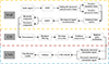 |
Figure 1. The flowchart of HPSS-CIS and CNN-CBAM. |
2 Methodology
The proposed methodology's flowchart is illustrated in Figure 1.
The complete process consists of five parts, each of which is explained separately in subsequent subsections. Firstly, the collected original audio signal to be diagnosed is decomposed into harmonic components and percussion components by the HPSS algorithm. Next, both components are processed by the CIS algorithm to transform them into multichannel electrode stimulation signals. Finally, the obtained electrode stimulation signals were classified and diagnosed using the constructed deep learning model of CNN-CBAM.
2.1 NMF-based HPSS
Harmonic Percussive Source Separation (HPSS) processing can separate the different components of sound signal and enhance fault manifestation, which will be more conducive to the detection and classification of heterophonic signals. According to the anisotropy assumption of harmonic signals and percussive signals, it is considered that the spectrum of harmonic component has harmonic and sparse structure in frequency dimension and is harmonic in temporal dimension. Correspondingly, the spectrum of impulse component has opposite characteristics in two dimensions. In recent years, the preprocessing method of separating speech has obtained good recognition results in audio classification models.
Lee and Seung introduced the multiplicative update rule of NMF for KL divergence [28]. As we iteratively update the parameters in NMF approach, a non-negative matrix which is a time-frequency spectrogram of STFT in this paper, can be represented as a multiplication operation of two non-negative submatrices that are denoted as spectral bases and temporal bases respectively:
 (1)
(1)
where, F represents the M×N spectrogram of the original signal, W represent the M×K spectral base matrix, H represent the K×N activation matrix, K represents the number of base vectors.
The update rule can be represented as:
 (2)
(2)
 (3)
(3)
where,  represents the estimated spectrogram.
  represent the estimated spectral base matrix,
  represent the estimated activation matrix. Wm,k represents the element at the mth row and kth column of the W matrix, and the same applies to Hk,n, Fm,n,
  ,
,  ,
,  .
.
According to the Dirichlet prior, equations (2) and (3) are updated to a weighted sum form with hyperparameters. The weighted sum formula is added to the update equations of standard non-negative matrix factorization, and the update equation for the activation matrix is as follows:
![Mathematical equation: $$ {{\hat {H}}}_{k,n}^{H} \leftarrow \alpha {\widetilde {H}}_{k,n}^{H} + \left ({1 - \alpha } \right ){\widetilde {H}}_{k,n - 1}^{H},\ n \in \left [ {1,N} \right ] $$](/articles/aacus/full_html/2025/01/aacus240138/aacus240138-eq10.gif) (4)
(4)
![Mathematical equation: $$ {{\hat {H}}}_{k,n}^{P} \leftarrow \beta {\widetilde {H}}_{k,n}^{P} + \left ({1 - \beta } \right ){\widetilde {H}}_{k,n - 1}^{P},\ n \in \left [ {1,N} \right ] $$](/articles/aacus/full_html/2025/01/aacus240138/aacus240138-eq11.gif) (5)
(5)
 (6)
(6)
where,  represents the estimated harmonic activation matrix during the update process,
  represent the estimated percussive activation matrix during the update process. α and β represents the weighting factors.
Correspondingly, the spectral basis matrix update equation is as follows:
![Mathematical equation: $$ {{\hat {W}}}_{m,k}^{H} \leftarrow \gamma {\widetilde {W}}_{m,k}^{H} + \left ({1 - \gamma } \right ){\widetilde {W}}_{m - 1,k}^{H},\ m \in \left [ {1,M} \right ] $$](/articles/aacus/full_html/2025/01/aacus240138/aacus240138-eq15.gif) (7)
(7)
![Mathematical equation: $$ {{\hat {W}}}_{m,k}^{P} \leftarrow \delta {\widetilde {W}}_{m,k}^{P} + \left ({1 - \delta } \right ){\widetilde {W}}_{m - 1,k}^{P},\ m \in \left [ {1,M} \right ] $$](/articles/aacus/full_html/2025/01/aacus240138/aacus240138-eq16.gif) (8)
(8)
 (9)
(9)
where,  represents the estimated harmonic spectral base matrix during the update process,
  represent the estimated percussive spectral base matrix during the update process. γ and δ represents the weighting factors.
Weighting factors are used to suppress or amplify differences between adjacent elements to enhance continuity and sparsity, and a weighting factor higher than 1 increases the variability. Based on the discontinuity principle of the spectral base of the shock component and temporal base of the harmonic components, β and γ are set to be higher than 1, and α and δ are set to be less than 1 to smooth the fluctuation of each basis matrix of the iterative process. After one iteration, the estimation spectrogram of harmonic component and the shock component are reconstructed by the following equation:
 (10)
(10)
 (11)
(11)
The spectrogram of the harmonic component and the shock component are obtained after several iterations of the above process, and then the audio signals of the harmonic and shock components are obtained by the inverse Fourier transform.
2.2 The algorithm of CIS
The CIS algorithm of Cochlear implant, which has high reliability and visualization as a simulation of human hearing, can provide deaf people with the ability to restore a certain level of hearing function, and has been widely used in real-life situations.
Wilson et al. put forward the continuous interval sampling scheme (CIS) in 1991 to overcome the mutual interference between channels caused by simultaneous stimulation of the CA coding scheme [29]. In this paper, we perform CIS processing on each of the two components obtained from the raw signals after HPSS pre-separation in order to convert them into multichannel electrode stimulation signals that satisfy the auditory perception of the human ear. The main processes are shown below:
Step 1.:
The audio signal component is input into the Chebyshev II filter to obtain filtered signals of different frequency bands; The central frequency of each band corresponds to the frequency position of the stimulation electrode on the cochlear basement membrane to simulate the frequency distribution function of the human ear. The frequency band distribution of the filter is given by the Greenwood cochlear frequency-position function, and the formula is as follows:
 (12)
(12)
where f corresponds to the cochlear frequency point, A and k are constants, and L is the position from the top of the cochlear basement membrane, which α is a constant coefficient related to the position L. In this paper, the value of A is 165.4, the value of k is 2.1.
Step 2.:
Hilbert-transform and low-pass filter are used to convert the filtered signals with different frequencies into envelope signals, and the cut-off frequency of each channel is 200 Hz; In order to meet the requirements of cochlear stimulation threshold, the extracted envelope is then limited by a low-pass filter. The filter is a third-order Butterworth type with a cut-off frequency of 200 Hz. The following formula is envelope signal extraction:
 (13)
(13)
 (14)
(14)
where, x(t) is the input signal,  is the Hilbert transform of x(t), y(t) is the envelope signal.
Step 3.:
Due to the limitation of the dynamic range, the envelope signal of each channel is nonlinearly compressed to improve the dynamic range of the envelope value of the sub-band envelope signal; Logarithmic compression is adopted to realize the dynamic range mapping of acoustic electric amplitude and simulate the auditory range generated by the amplitude of electrical stimulation.
 (15)
(15)
where, Y(t) is the nonlinear compressed envelope signal, C and D are constants respectively, which are used to limit the compressed sound amplitude Y between the lowest auditory threshold level and the maximum comfortable auditory level.
Step 4.:
Biphase-pulse modulation is performed on the compressed envelope signal Y(t) to obtain the stimulation electrode signal. A two-phase matrix window of N points is defined as follows:
 (16)
(16)
 (17)
(17)
where, N is the biphasic matrix pulse window length, ω(n) is the unit biphasic matrix pulse,  is the electrode stimulation signal, T is the pulse rate (the number of pulses within 1 s).
2.3 CNN-CBAM
The convolutional neural network (CNN) is a type of feedforward neural network that utilizes convolutional computation and depth structure. The sharing of parameters in the convolution kernel within the hidden layer of the CNN and the sparse connections between layers facilitate the learning of lattice features, including pixels and audio, by the convolutional neural network. This is achieved with minimal computation, yielding stable results and requiring no extraneous feature engineering for the data.
The widely used classical CNN module mainly consists of a convolutional layer, a pooling layer and an activation function. The convolution layer operates by using a consistent convolution kernel to traverse the input with a fixed step size. At each traversed location, the convolution kernel and the neuron of the previous layer perform convolution operations. The calculation formula is specific and as follows:
 (18)
(18)
where, w is the weight of convolution kernel, x is the convolution region of the starting point.
The main function of pooling layer is to concentrate the feature map. In order to effectively remove a large amount of irrelevant noise information from the time domain signal, maximum pooling is chosen to filter the features and speed up the computation. The activation function is a nonlinear function, which can perform nonlinear transformation on the input value to enhance the network's ability to express nonlinearity. The ReLU function, also known as the linear correction unit, is now the most widely used formula in the field of machine learning, and is also the choice of this paper.
 (19)
(19)
When technicians perform manual listening tests on factory motors, they do not usually focus their attention all the time to analyze seriously the long-term smooth noise of the motor. Only when the motor suddenly makes an abnormal sound, the human ear will focus on the sudden change in sound and identify the fault of the motor. And the attention mechanism allows the neural network to selectively focus on the important information in the input, improving the performance and generalization of the model.
CBAM is a lightweight convolutional attention module that can be embedded into CNNs to enhance the network's representational and perceptual capabilities, and it contains two sub-modules, the channel attention module and the spatial attention module [30]. In the convolutional neural network, given an intermediate feature map input, CBAM derives the channel attention and spatial attention sequentially, and then multiplies the attention weight matrix with the input feature map for adaptive feature refinement. The structure of a complete CNN-CBAM block is shown in Figure 2.
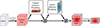 |
Figure 2. The structure of CNN-CBAM block. |
2.4 Evaluation metrics
To evaluate the performance of the model, accuracy, recall, specificity, precision, and F1 score are used the indicator formulas are as follows:
 (20)
(20)
 (21)
(21)
 (22)
(22)
 (23)
(23)
where, TP is true positive, FP is false positive, FN is false negative, and TN is true negative.
Accuracy indicates the ratio of samples whose predictions match the label to the total sample. Precision characterizes the ability of the classification model to return only relevant instances. Recall represents the ability of the classification model to identify all relevant instances. F1-score is a reconciled average of precision and recall.
3 Experimental procedure
3.1 Data acquisition
The experimental data in this paper comes from motors with abnormal sound faults accumulated during the production process of the factory motor production line. The technicians set up the labels according to the type of motor noises after manual listening and collected samples of the audio signal using microphone sensors.
The experiment was conducted in the semi-anechoic chamber of the factory motor assembly line, and the acquisition device is shown in Figure 3. The type of motor to be tested is brushless direct current motor, the rated voltage is 220 V, the rated power is 33 W, and the speed is 1000 r/min. The two microphone sensors are used to collect the sound signals from the motor during normal operation, and the microphone sensors are located within a range of about 10 cm from the motor to achieve the collection of sound signals from the motor. The sampling time is 1 s, and the sampling frequency of sensor is 23 759 Hz. The motor bearing model is 6202 SKF with the rotational frequency of the output shaft as the 1st order frequency, the characteristic order of bearing failure is shown in Table 1.
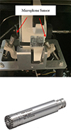 |
Figure 3. Signal acquisition test stands and microphone sensors. |
Air-conditioner motor bearing failure order.
The abnormal noise from the air conditioning motor mainly comes from improper processing of internal components and assembly processes, such as rotor imbalance, bearing failure, and foreign objects entering the motor cavity. In the dataset obtained from the test, the labels of the good motor operation sound signal samples are noted as ZC, totaling 132 pieces, and the labels of the abnormal sound samples are noted as YC, totaling 428 pieces, where YC contains four types. The five types of typical sound signals are shown in Figure 4. And the auditory perception, signal frequency characteristics and number of each type of signal are shown in Table 2.
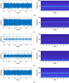 |
Figure 4. The five types of typical sound signals. (a) ZC. (b) YC1. (c) YC2. (d) YC3. (e) YC4. |
The dataset of five types of different sounds.
In the field of psychoacoustics, fluctuation and roughness can be used to describe the amplitude change of noise perceived by the human ear resulting from modulation. Fluctuating sounds are used to describe the phenomenon of jittery sound perceived by the human ear during slow modulation at modulation frequencies less than 20 Hz. Rough sounds reflect the sound produced by rapid modulation at frequencies in the range of 20–200 Hz, which the human ear cannot directly perceive as temporal fluctuations of the signal. YC1 is a periodic fluctuating sound that is slowly modulated by the motor's rotational frequency, YC2 is a periodic shock sound of the 2nd order rotational frequency, YC3 is a rough sound of rapid modulation caused by bearing outer ring failure, and YC4 (Whistling sound) is a high-frequency harmonic sound.
3.2 Feature extraction
Time-frequency analyses of typical abnormal sound signals show that the abnormal features are mainly reflected in the harmonic and shock components of the signals. Pre-extraction of harmonic and percussive components of the sound signal will contribute to the diagnostic and classification tasks of abnormal sounds.
Next, an actual motor audio signal is processed by HPSS. FFT window length is 256 sampling points, frame shift is 128 sampling points, and window function is Hamming window. The maximum number of iterations is 100. α, β, γ, and δ is set to 0.7, 1.1, 1.05, and 0.9, respectively.
An actual motor audio signal is separated into harmonic and percussive components as shown in Figure 5. The NMF-based HPSS algorithm can effectively separate the harmonic components and shock components in the original signal of motor abnormal sound, and the sub-components will be used for further signal processing.
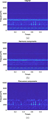 |
Figure 5. Time frequency diagram after NMF algorithm decomposition. (a) Original signal. (b) Harmonic component. (c) Percussive component. |
Next, the five types of motor sound signals were processed by HPSS-CIS to obtain electrode stimulation signals. The number of frequency channels is 10, and the range of frequency f is 500–10 000 Hz, the results of frequency band division calculated according to equation (12) are shown in Table 3.
Frequency band division.
The biphasic matrix pulse rate (the number of pulses within 1 s) is set to be 1000 pps, and the window length was 2 points. The electrode stimulation signals for the five types of sounds are shown in Figure 6.
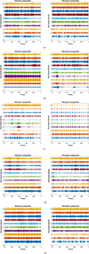 |
Figure 6. Five types of electrical stimulation signals after HPSS-CIS. (a) ZC. (b) YC1. (c) YC2. (d) YC3. (e) YC4. |
In the five signals shown, we can see that: YC1 has clear modulated harmonics in bands 1–5 of the harmonic component relative to ZC; the abnormal features of YC2 are mainly shown in the percussion component; YC3 has clear rapid modulated signal, in bands 2–4 of the harmonic component and bands 3, 4 of the percussion component; compared to ZC, YC4 has the smoother component in the harmonic band where the abnormal sound occurs, e.g., bands 1, 3, and 10 of the harmonic components in Figure 6e. We can visually distinguish between different heterophonic types using the output electrode stimulation signals and the results are interpretable.
4 Comparative analysis of model effectiveness
In this study, we use the HPSS-CIS algorithm to simulate the transformation process of sound signals during the input of motor sounds through the human cochlea to the neural process of the brain, and use the neural network model of CNN-CBAM to learn the black-box process of the brain on the electrical stimulation signals, in order to realize as much as possible the consistent decision-making between humans and machines on the same sound signals. The whole process of the test is as follows:
Step 1.: The audio signals of all motors operating at rated speeds were collected in a semi-anechoic chamber, while professionals listened and recorded labels for each sample;
Step 2.: The motor audio signal is separated from the harmonic impulse to obtain harmonic signal components and impulse signal components;
Step 3.: The harmonic component and impulse component are processed by CIS algorithm respectively to obtain electric pulse stimulation signal;
Step 4.: The multichannel electrode stimulated signals were used as inputs to the CNN-CBAM network. And 75% of the dataset is used for model training;
Step 5.: Evaluate model performance using the test set.
Concretely, the HPSS-CIS algorithm parameters are described in Section 3.2. After data acquisition and feature extraction, a classification model based on deep learning is constructed for the intelligent detection of abnormal motor sounds. The original abnormal sound signals of motor faults were transformed into 20-channel time-domain features after HPSS and CIS processing, which were inputted into the model of CNN-CBAM for training and testing. The parameters of the constructed CNN-CBAM model are shown in Figure 7. As shown in Table 2, the dataset contains 560 samples. 75% of the dataset will be divided as the training set, and the remaining 25% as the test set. After signal processing of the samples, the training set is inputted into the neural network to train to get the classification model. The Adam optimizer is used to iterate the network parameters, the number of iterations is set to 250, and learning rate is 0.001 and the dropout of the model parameters set to 0.2.
 |
Figure 7. The Architect of CNN-CBAM model. |
In order to set the appropriate number of model parameters, a grid search method was used for the 1D convolution kernel size and the number of channels. The convolution kernel size ranges from [4,8,16,32] and the number of channels ranges from [8,16,32,64], and each parameter configuration is repeated 5 times to take the average accuracy as the performance of the model, and the results are shown in Figure 8.
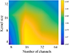 |
Figure 8. Grid search to find optimal model parameter settings. |
Taking the best parameter hyperparameters for model training, we obtained a model that can be used to classify abnormal motor sounds. And this model is used to predict the classification results of the test set, and showed satisfactory performance. Of the 140 test set samples, 33 samples labeled ZC were normal motors, and 107 samples labeled YC were motors that contained abnormal noises. The accuracy of the proposed method is up to 99.27%. Of all the samples in the test set, only one anomaly sample was misclassified as another anomaly label, and there was no case of false alarm, which satisfied the industrial actual needs of motor production, and the confusion matrix for the classification results is shown in Figure 9.
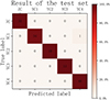 |
Figure 9. The optimal classification results of the proposed method. |
In order to evaluate the contribution of all components of the proposed method, we performed comparative experiments on each of the two parts, the audio signal processing methods and the deep learning models.
The ablation test of the HPSS-CIS method was performed to analyze the contribution of each single component to the diagnosis of abnormal sound. In the ablation experiments of the HPSS-CIS algorithm, the entire algorithm was subjected to three treatments of removing the HPSS-CIS algorithm, removing the CIS algorithm, and removing the HPSS algorithm, which are equivalent to using the time-domain features, the features of HPSS, and the features of CIS inputted into a deep learning model to make a prediction and compared with the HPSS-CIS, respectively.
All the processed features are inputted into the CNN-CBAM model, and all models were set to the optimal hyperparameters. Each model was trained on train set and predicted on the test set ten times, and the indicators of evaluation were averaged as the performance of that method.
The results of method ablation test are shown in Table 4. After using the HPSS algorithm and the CIS algorithm, the average accuracy of the model increased by 2.21% and 1.43%, respectively, compared to the original time-domain signal, while the score of remaining three indicators were also improved. Meanwhile, the HPSS-CIS method, which combines two signal processing methods, has optimal performance in all four evaluation metrics, and improves the average accuracy of the model by more than 4.5% compared to any single component.
Method ablation test of the HPSS-CIS.
Two widely used current sound feature extraction methods in speech recognition, i.e., Mel-frequency cepstral coefficients (MFCC) [31] and Mel-spectrogram [32], utilize the Mel filter bank and Mel scale to simulate the nonlinear frequency response of the human ear auditory system. Mel frequency conversion equation is as follows:
 (24)
(24)
where, f is linear frequency/Hz.
Therefore, the Mel filter bank method was chosen for comparison with the CIS method used in this paper. The separated components of HPSS are processed separately with Mel filter bank, and the output features are noted as HPSS-Mel.
Consistent with the previous ablation experiment, the optimal hyperparameters were chosen for models of all kinds of features. Each model was trained on train set and predicted on the test set ten times, and the indicators of evaluation were averaged as the performance of that feature. The results of each method are shown in Table 5.
Performance of different audio feature extraction methods.
As shown in Table 5, the HPSS-CIS method shows the best performance in all four indicators of evaluation, compared to HPSS-Mel. And relatively, the average misclassification rate was decreased from 4.73% to 2.29%. This is very meaningful for the classification of motor noises in industry.
Finally for model selection, we selected Bi-GRU (Bidirectional Gate Recurrent Unit) and classical CNN model to compare with the CNN-CBAM model, under four different prediction metrics. The gated recurrent unit (GRU) is evolved from the LSTM and continues the long-time temporal memory capability of the LSTM while speeding up the computation. Meanwhile, the bidirectional GRU structure can extract both forward and backward information to find the underlying temporal relationship of the signal more accurately. The comparison of GRU with CNN and its variants allows for a better determination of which neural network framework is more effective for abnormal sound diagnosis in this paper. On the other hand, the effectiveness of CBAM can be fully demonstrated by comparing CNN-CBAM with classical CNNs.
In the experiment, the training set and test set are randomly divided for the training and testing of the three models. The process is repeated ten times, and the average of the evaluation metrics for each model is used to characterize the performance of that model. The results for all deep learning models are shown in Table 6.
Performance comparison of three deep learning models.
As shown in Table 6, the Bi-GRU model has the lowest scores on four evaluation metrics, and its average accuracy is reduced by more than 23.71% compared to CNN and CNN-CBAM. And with the introduction of the CBAM attention mechanism, the average accuracy of the CNN model increases by 4.14%, and achieves the most superior results in all four evaluation indicators, which verifies the validity of the chosen model of CNN-CBAM.
5 Conclusion
In this paper, a method based on HPSS-CIS and CNN to detect and classify the abnormal sound of air conditioning motor is proposed. The collected motor audio signal is decomposed into harmonic component and impact component by non-negative matrix, and the two components are processed into electrode stimulation signals of each frequency division band by cochlear implant CIS algorithm. The frequency division conforms to the nonlinearity of cochlea. Combined with CNN's powerful voice signal processing capability and attentional mechanism of CBAM, the highest accuracy of abnormal sound classification can reach up to 99.27% on the obtained dataset through experiments, which result can meet the engineering requirements.
Ablation tests of the HPSS-CIS verify that, the HPSS-CIS method which combines two signal processing methods improves the average accuracy of the model by more than 4.5% compared to any single component. Meanwhile, for the human auditory feature extraction method after HPSS processing, the CIS method is compared with the widely used Mel filter bank in this paper, and shows superior performance in all four indicators of evaluation, the average misclassification rate was decreased from 4.73% to 2.29%. Finally, the effectiveness of the constructed CNN-CBAM model is verified by comparing with CNN and Bi-GRU models.
In addition to providing an automated solution for the detection and categorization of motor noises, this study also provides an engineering idea to guide product quality control and improvement based on the user's auditory perception rather than the direct type of fault, which may have promising applications in other types of motors, engines, and other devices that may cause serious noise impacts on the user's experience, in addition to the motor types mentioned in this paper. The current results of the method presented in this paper are based on heterodyne data of the same type of air conditioning motors, and the sample size of the dataset is small, thus making it difficult to thoroughly argue for the generalizability of the study's conclusions. This problem can also be solved by obtaining more data samples for optimization in the future.
Funding
This work supported by the Joint Funds of the National Natural Science Foundation of China (Grant No. U2267206) and State Key Laboratory of Manufacturing System Engineering in Xi’an JiaoTong University.
Conflicts of interest
The authors declare that they have no known competing financial interests or personal relationships that could have appeared to influence the work reported in this paper.
Data availability statement
Our data comes from Guangdong Midea Refrigeration Equipment Co., Ltd. China. We have signed a confidentiality agreement, so we cannot share data.
References
- R. El Idrissi, A. Bacha, F. Lmai: Fault diagnosis using Bayesian networks for a single-phase inverter based on MOSFET semiconductors. Materials Today: Proceedings (2024). https://doi.org/10.1016/j.matpr.2024.01.043 [Google Scholar]
- P. Kundu: Review of rotating machinery elements condition monitoring using acoustic emission signal. Expert Systems with Applications 252 (2024) 124169 [CrossRef] [Google Scholar]
- P.A. Delgado-Arredondo, D. Morinigo-Sotelo, R.A. Osornio-Rios, J.G. Avina-Cervantes, H. Rostro-Gonzalez, R. de Jesus Romero-Troncoso: Methodology for fault detection in induction motors via sound and vibration signals. Mechanical Systems and Signal Processing 83 (2017) 568–589 [CrossRef] [Google Scholar]
- A.D. Barman, S. Mondal: Experiment on spectrogram feature based CNN for sound anomaly detection, in: 2023 8th International Conference on Computers and Devices for Communication (CODEC). IEEE, 2023, pp. 1–2 [Google Scholar]
- A. Altinors, F. Yol, O. Yaman: A sound based method for fault detection with statistical feature extraction in UAV motors. Applied Acoustics 183 (2021) 108325 [CrossRef] [Google Scholar]
- S. Lu, X. Wang, Q. He, F. Liu, Y. Liu: Fault diagnosis of motor bearing with speed fluctuation via angular resampling of transient sound signals. Journal of Sound and Vibration 385 (2016) 16–32 [CrossRef] [Google Scholar]
- E. Germen, M. Başaran, M. Fidan: Sound based induction motor fault diagnosis using Kohonen self-organizing map. Mechanical Systems and Signal Processing 46 (2014) 45–58 [CrossRef] [Google Scholar]
- S.S. Ahmed, A.M. Gadelmoula: Industrial noise monitoring using noise mapping technique: a case study on a concrete block-making factory. International Journal of Environmental Science and Technology 19 (2022) 851–862 [CrossRef] [Google Scholar]
- J. Son, C. Kim, M. Jeong: Unsupervised learning for anomaly detection of electric motors. International Journal of Precision Engineering and Manufacturing 23 (2022) 421–427 [CrossRef] [Google Scholar]
- A. Suman, C. Kumar, P. Suman: Early detection of mechanical malfunctions in vehicles using sound signal processing. Applied Acoustics 188 (2022) 108578 [CrossRef] [Google Scholar]
- M. Chuphal, K. Singh, A. Bisht, V. Sharma, S. Awasthi, S. Vats: Anomaly detection in electro-mechanical devices using MFCC, in: 2024 2nd International Conference on Disruptive Technologies (ICDT). IEEE, 2024, pp. 986–991 [Google Scholar]
- M.S. Sidhu, N.A.A. Latib, K.K. Sidhu: MFCC in audio signal processing for voice disorder: a review. Multimedia Tools and Applications 84 (2025) 8015–8035 [Google Scholar]
- A.J. Torija, Z. Li, P. Chaitanya: Psychoacoustic modelling of rotor noise. The Journal of the Acoustical Society of America 151 (2022) 1804–1815 [CrossRef] [PubMed] [Google Scholar]
- F.C. Hirono, J. Robertson, A.J.T. Martinez: Acoustic and psychoacoustic characterisation of small-scale contra-rotating propellers. Journal of Sound and Vibration 569 (2024) 117971 [CrossRef] [Google Scholar]
- E. Zwicker, H. Fastl: Psychoacoustics: Facts and Models. Vol. 22. Springer Science & Business Media, 2013 [Google Scholar]
- M. Yüksel, O. Önen, B.U. Seeber: Acoustics, psychoacoustics, and properties of sound, in: Otology Updates. Springer Nature Switzerland, Cham, 2025, pp. 113–124 [Google Scholar]
- J. Park, K. Lee: Harmonic-percussive source separation using harmonicity and sparsity constraints, in: ISMIR, 2015, pp. 148–154 [Google Scholar]
- C. Uhle, C. Dittmar, T. Sporer: Extraction of drum tracks from polyphonic music using independent subspace analysis, in: Proc. ICA., 2003, pp. 843–847 [Google Scholar]
- O. Gillet, G. Richard: Drum track transcription of polyphonic music using noise subspace projection, in: ISMIR, 2005, pp. 92–99 [Google Scholar]
- M. Helen, T. Virtanen: Separation of drums from polyphonic music using non-negative matrix factorization and support vector machine, in: 2005 13th European Signal Processing Conference. IEEE, 2005, pp. 1–4 [Google Scholar]
- M. Kim, J. Yoo, K. Kang, S. Choi: Nonnegative matrix partial co-factorization for spectral and temporal drum source separation. IEEE Journal of Selected Topics in Signal Processing 5 (2011) 1192–1204 [CrossRef] [Google Scholar]
- J.J. Carabias-Orti, T. Virtanen, P. Vera-Candeas, N. Ruiz-Reyes, F.J. Canadas-Quesada: Musical instrument sound multi-excitation model for non-negative spectrogram factorization. IEEE Journal of Selected Topics in Signal Processing 5 (2011) 1144–1158 [CrossRef] [Google Scholar]
- D. Fitzgerald: Harmonic/percussive separation using median filtering, in: 13th International Conference on Digital Audio Effects (DAFX10), Graz, Austria, 2010 [Google Scholar]
- F.D. González-Martínez, J.J. Carabias-Orti, F.J. Cañadas-Quesada, N. Ruiz-Reyes, D. Martínez-Muñoz, S. García-Galán: Improving snore detection under limited dataset through harmonic/percussive source separation and convolutional neural networks. Applied Acoustics 216 (2024) 109811 [CrossRef] [Google Scholar]
- T. Zhao, W. Ding, H. Huang, Y. Wu, Adaptive multi-feature fusion for vehicle micro-motor noise recognition considering auditory perception. Sound and Vibration 57 (2023) 133–153 [CrossRef] [Google Scholar]
- P. Gonzalez, G. Buigues, A.J. Mazon: Noise in electric motors: a comprehensive review. Energies 16 (2023) 5311 [CrossRef] [Google Scholar]
- A. Dhanasingh, I. Hochmair: Signal processing & audio processors. Acta Oto-Laryngologica 141 (2021) 106–134 [CrossRef] [Google Scholar]
- D. Lee, H.S. Seung: Algorithms for non-negative matrix factorization, in: Advances in Neural Information Processing Systems. Vol. 13. MIT Press, 2000 [Google Scholar]
- B.S. Wilson, D.T. Lawson, M. Zerbi, C.C. Finley, R.D. Wolford: New processing strategies in cochlear implantation. Otology & Neurotology 16 (1995) 669–675 [Google Scholar]
- J. Qin, S. Zhang, Y. Wang, F. Yang, X. Zhong, W. Lu: Improved skeleton-based activity recognition using convolutional block attention module. Computers and Electrical Engineering 116 (2024) 109231 [CrossRef] [Google Scholar]
- X. Hu, J. Lou, T. Chen, J. Ma, G. Li: Quality evaluation method of the DC motor based on VMD and MFCC, in: 2023 China Automation Congress (CAC). IEEE, 2023, pp. 1710–1714 [Google Scholar]
- S. Shan, J. Liu, S. Wu, Y. Shao, H. Li: A motor bearing fault voiceprint recognition method based on Mel-CNN model. Measurement 207 (2023) 112408 [CrossRef] [Google Scholar]
Cite this article as: Zhao Q. Wang X. Luo K. He D. & Liu X. 2025. Abnormal noise detection of electric machines based on HPSS-CIS and CNN-CBAM. Acta Acustica, 9, 39. https://doi.org/10.1051/aacus/2025023.
All Tables
All Figures
|
Figure 1. The flowchart of HPSS-CIS and CNN-CBAM. |
| In the text | |
|
Figure 2. The structure of CNN-CBAM block. |
| In the text | |
|
Figure 3. Signal acquisition test stands and microphone sensors. |
| In the text | |
|
Figure 4. The five types of typical sound signals. (a) ZC. (b) YC1. (c) YC2. (d) YC3. (e) YC4. |
| In the text | |
|
Figure 5. Time frequency diagram after NMF algorithm decomposition. (a) Original signal. (b) Harmonic component. (c) Percussive component. |
| In the text | |
|
Figure 6. Five types of electrical stimulation signals after HPSS-CIS. (a) ZC. (b) YC1. (c) YC2. (d) YC3. (e) YC4. |
| In the text | |
|
Figure 7. The Architect of CNN-CBAM model. |
| In the text | |
|
Figure 8. Grid search to find optimal model parameter settings. |
| In the text | |
|
Figure 9. The optimal classification results of the proposed method. |
| In the text | |
Current usage metrics show cumulative count of Article Views (full-text article views including HTML views, PDF and ePub downloads, according to the available data) and Abstracts Views on Vision4Press platform.
Data correspond to usage on the plateform after 2015. The current usage metrics is available 48-96 hours after online publication and is updated daily on week days.
Initial download of the metrics may take a while.