| Issue |
Acta Acust.
Volume 9, 2025
|
|
|---|---|---|
| Article Number | 38 | |
| Number of page(s) | 16 | |
| Section | Acoustic Materials and Metamaterials | |
| DOI | https://doi.org/10.1051/aacus/2025022 | |
| Published online | 25 June 2025 | |
Scientific Article
Derivation, verification and validation of a length correction factor for folded quarter-wavelength resonators
1
KU Leuven, Department of Mechanical Engineering, Division LMSD Wetenschapspark 27 3590 Diepenbeek Belgium
2
Flanders Make@KU Leuven Leuven Belgium
3
KU Leuven, Department of Mechanical Engineering, Division LMSD Celestijnenlaan 300B 3001 Leuven Belgium
* Corresponding author: This email address is being protected from spambots. You need JavaScript enabled to view it.
Received:
28
December
2024
Accepted:
16
May
2025
Abstract
Acoustic metamaterials that consist of multiple λ/4-resonators in series or parallel can be tuned to realise high broadband absorption in a given frequency range. These resonators are often folded to obtain a structure with a (deep) sub-wavelength thickness, which allows an optimal use of the available space and enables low-frequency sound absorption in confined spaces. However, folding a resonator can lead to a significant change in resonance frequency, resulting in an off-design acoustic performance. Hence, in this paper, the effect of a single 90° fold on the resonance frequency of rectangle and slit-like λ/4-resonators is investigated numerically. Based on these numerical simulations, a length correction factor δ is derived to account for this effect in the analytical model. The use of the correction factor is verified for various single-fold resonator configurations and against existing length formulas. The length correction factor is then experimentally validated for rectangle resonators by means of impedance tube measurements on 3D printed samples. It is found that using the proposed length correction factor allows for an accurate prediction of the resonance frequency of the discussed resonator geometries.
Key words: Acoustic metamaterial / Quarter-wavelength resonator / Folding / Length correction factor / 3D printing
© The Author(s), Published by EDP Sciences, 2025
 This is an Open Access article distributed under the terms of the Creative Commons Attribution License (https://creativecommons.org/licenses/by/4.0), which permits unrestricted use, distribution, and reproduction in any medium, provided the original work is properly cited.
1 Introduction
To meet indoor noise regulations, sound abatement techniques that intervene at the transfer path are widely applied. An example of such techniques are sound absorbing panels, which lower the indoor sound pressure level by reducing the intensity of the reflected sound waves. These panels commonly consist of either porous layers (e.g. mineral wool) or resonance-based absorbers (e.g. Helmholtz-, λ/2- and λ/4-resonators). However, since the needed layer thickness or resonator length scales with the wavelength [1–4], conventional sound absorbing panels become bulky when targeting low-frequency sound, which poses issues in confined spaces such as vehicle interiors and airplane cabins.
In order to provide a high-performing and space-efficient solution to low-frequency sound problems, academic research has been focussing on acoustic metamaterials (AMMs), which exploit the same physical principles as conventional sound absorbing structures, but are characterized by a more complex geometry, which enables them to realise high absorption while maintaining a (deep) sub-wavelength thickness [5–36].
A commonly used type of AMMs are folded quarter-wavelength acoustic metamaterials (QW-AMMs), which can consist of solely folded λ/4-resonators (usually in a parallel assembly) or can be a combination of a folded λ/4-resonator and other absorber concepts [6–21].
The acoustic performance of such QW-AMMs can be modelled using either computationally extensive finite element simulations or an analytical model. This model requires several inputs, including the effective resonator length.
How this length must be calculated depends on the resonator's folding layout. For labyrinth folded λ/4-resonators, a distinction is made based on the assumed sound propagation path. If the sound waves are assumed to propagate along a zigzag path, as in a.o. [7–14, 19], the effective resonator length can be calculated using Pythagoras’ theorem. If the sound waves are assumed to propagate along a circular path near the fold, the effective length is calculated as the sum of the centreline length and a correction factor [20]. For λ/4-resonators with separate 90° folds, things are less straightforward: for this type of resonators, no consensus is found in literature on how the effective length must be calculated. For example, Zhang Z. et al. propose in [21] to assume the effective length equal to the centreline length. However, the accuracy of this approach is found to largely depend on the resonator layout. In hindsight, an adapted version of the formula presented in [20] could have been applied, but also the accuracy of this approach is expected to be highly dependent on the folding layout since this present formula does not account for the nearness of the fold to the resonator opening, although this parameter is found to be important [37]. In [18], on the other hand, Qinhao, L. and Guoqing, D. applied Pythagoras’ theorem to calculate the effective resonator length. However, it is unclear how the trajectory within each channel is determined. Additionally, the effective length of some channels is greater than the centreline length, which is not in line with the experimental findings in a.o. [21]. Lastly, one can also attempt to calculate the effective length of λ/4-resonators with separate 90° folds by combining the aforementioned formulas, as done in [17]. In their work, Wang Y. et al. propose a length formula which combines the Pythagoras’ theorem, the centreline assumption and a correction factor. Although good agreement between the analytical and numerical results is found, it is unclear on which physics the assumed sound propagation path and proposed length correction are based.
Due to the issues with determining the effective resonator lengths, QW-AMMs that consist of λ/4-resonators with separate 90° folds are barely studied in literature. This is unfortunate, since these structures show much potential, as shown in [21]. They also offer a larger freedom of design as compared with labyrinth folded resonators and, thus, lend themselves better for optimal use of the available space, which might result in a better acoustic performance. Hence, to facilitate the design and encourage further development of this type of QW-AMMs, this paper takes first steps towards the definition of a formula to calculate the effective length of a λ/4-resonator with separate 90° folds by (i) investigating the effect of a single 90° fold on the effective length of rectangle and slit-like λ/4-resonators and (ii) deriving a length correction factor δ to account for this effect into the analytical model, similar to as performed by Cambonie T. et al. for a bent resonator and by Catapane G. et al. for labyrinth resonators [20, 38]. The eventual expression for δ is verified numerically and experimentally validated.
The remainder of this paper is structured as follows. In Section 2, the basic analytical model used to predict the absorption coefficient of rectangular and slit-like λ/4-resonators is explained. Section 3 covers the stepwise derivation of δ and the numerical verification of δ against other single-fold resonator configurations and state-of-the-art length (correction) formulas. In Section 4, the experimental validation of δ by means of impedance tube measurements on 3D printed samples is discussed. Section 5 concludes this paper with an overview of the main results.
2 Analytical model
The effectiveness of a sound absorber is usually expressed in terms of the absorption coefficient α, which is defined as the ratio of the absorbed intensity to the incident intensity under normal incidence. This ratio can be rewritten in terms of impedances as given by equation (1):
 (1)
(1)
with ϱ0 the ambient density, c0 the ambient sonic speed and Ztot the input impedance of the sound absorber [3]. The frequency at which α reaches its maximum value is called the resonance frequency fR of the absorber. If the sound absorber consists of a single and rigid λ/4-resonator embedded in a finite baffle, Ztot is given by equation (2):
 (2)
(2)
with j the imaginary unit, Ab the cross-section area of the baffle, Ar the cross-section area of the resonator,  the impedance of the medium inside the resonator,
  the wavenumber of the sound waves inside the resonator, L′ the effective resonator length, ω the angular frequency and ɛ the so-called end correction used to account for 3D effects occurring at the resonator opening [2, 3, 39, 40]. If the sound absorber consists of multiple structures in parallel, Ztot can be calculated based on the electrical-acoustical analogy as given by equation (3):
 (3)
(3)
with Zr,i the input impedance of the i-th structure. For a QW-AMM consisting of i λ/4-resonators in parallel, Zr,i is given by equation (2).
2.1 Equivalent fluid parameters  and
and 
The parameters  and
and  out of equation (2) can be calculated using equations (4) and (5), respectively:
 (4)
(4)
 (5)
(5)
with  and
and  the bulk modulus and density of the medium inside the resonator, respectively [1]. Since the resonators considered in this work are narrow, as classified by Weston [41], significant visco-thermal losses will occur inside the resonators. These losses are accounted for in the calculation of
  and
and  .
.
For a rectangle resonator with cross-section 2w×2h,  and
and  are calculated using equations (6) and (7), respectively:
![Mathematical equation: $$ \begin{aligned}{\tilde {\varrho }} &= \frac {\eta w^2h^2}{j4\omega } \left [ \sum _{m=0}^{\infty }\sum _{n=0}^{\infty } \frac {1}{A_m^2 B_n^2\left (A_m^2 + B_n^2 + \frac {j\omega \varrho _0}{\eta }\right )} \right ] ^{-1}, \end{aligned} $$](/articles/aacus/full_html/2025/01/aacus240149/aacus240149-eq18.gif) (6)
(6)
![Mathematical equation: $$ \begin{aligned}{\tilde {K}} &= P_0\gamma \left [\gamma - (\gamma -1)\frac {j4\omega \varrho _{0}Pr}{\eta w^2h^2}\right . \\ &\quad \times \left .\sum _{m=0}^{\infty }\sum _{n=0}^{\infty } \frac {1}{A_m^2 B_n^2\left (A_m^2 + B_n^2 + \frac {j\omega \varrho _0Pr}{\eta }\right )} \right ]^{-1}, \end{aligned} $$](/articles/aacus/full_html/2025/01/aacus240149/aacus240149-eq19.gif) (7)
(7)
with A=(m+0.5)π/w, B=(n+0.5)π/h, η the dynamic viscosity of the medium, γ the specific heat ratio, Pr the Prandtl number and P0 the ambient pressure [42].
For a slit-like resonator (i.e. a rectangle resonator for which 2h≫2w),  and
and  are calculated using equations (8) and (9), respectively:
![Mathematical equation: $$ {\tilde {\varrho }} = \varrho _{0}\left [1 - \frac {\tanh (\beta \sqrt {j})}{\beta \sqrt {j}} \right ] ^{-1}, $$](/articles/aacus/full_html/2025/01/aacus240149/aacus240149-eq22.gif) (8)
(8)
![Mathematical equation: $$ {\tilde {K}} = P_{0}\gamma \left [1 + (\gamma - 1) \frac {\tanh (\beta \sqrt {jPr})}{\beta \sqrt {jPr}} \right ] ^{-1}, $$](/articles/aacus/full_html/2025/01/aacus240149/aacus240149-eq23.gif) (9)
(9)
with β =  [42].
[42].
2.2 End correction ɛ
The end correction for a rectangle or slit-like resonator embedded in a finite rectangle baffle with dimensions 2w′×2h′ can be calculated using equation (10) or equation (11), respectively:
![Mathematical equation: $$ \begin{aligned}\varepsilon _{R \subset R} &= \frac {4\xi \chi }{\pi } \sum _{mn^*}^{\infty } \nu _{mn}\left [\frac {\sin \left (m\pi \xi \right )}{m\pi \xi }\cdot \frac {\sin (n\pi \chi )}{n\pi \chi } \right ]^{2} \\ &\quad \times \left [\sqrt {\left (\frac {m}{w'} \right )^2 + \left (\frac {n}{h'} \right )^2} \right ]^{-1}, \end{aligned} $$](/articles/aacus/full_html/2025/01/aacus240149/aacus240149-eq25.gif) (10)
(10)
![Mathematical equation: $$ \varepsilon _{S \subset R} = \sum _{m=1}^{\infty } \frac {1}{m} \left [\frac {\sin \left (m\pi \xi \right )}{m\pi \xi } \right ] ^{2}, $$](/articles/aacus/full_html/2025/01/aacus240149/aacus240149-eq26.gif) (11)
(11)
with ξ=(2w)/(2w′) and χ=(2h)/(2h′) [40, 43]. Both equations (10) and (11) assume the resonator to be in the centre of the baffle.
2.3 Effective resonator length L′
The effective resonator length L′ is calculated differently depending on the resonator layout. For unfolded resonators, L′ equals the centreline length. For labyrinth folded λ/4-resonators, L′ is calculated using either Pythagoras’ theorem or the formula presented by Catapane G. et al. in [20]. For λ/4-resonators with separate 90° folds, however, no well-established approach to calculate the effective length is available in literature. In this work, steps are taken to fill this void. These steps are discussed in more detail in Section 3.
3 Derivation and verification of a length correction factor
In this paper, it is investigated if L′ of rectangle and slit-like λ/4-resonators with a single 90° fold can be expressed as L+δ with L the centreline length and δ a length correction factor, similar to as presented in [20]. To this end, three steps are taken:
-
The effect of a single 90° fold on the effective length of rectangle and slit-like λ/4-resonators is investigated by (i) modelling single-fold rectangle and slit-like λ/4-resonators numerically in COMSOL MultiPhysics® , (ii) extracting the resonance frequency fR of each resonator out of the simulation and (iii) calculating L′ from fR and comparing this value with L;
-
A length correction factor δ is defined as L′−L and a dimensionless expression for δ is derived through curve fitting;
-
The accuracy of δ is verified against arbitrary single-fold resonator configurations and existing length (correction) formulas.
Each of these steps is further elaborated on in the following subsections.
3.1 Numerical simulations in COMSOL MultiPhysics®
The numerical simulations are performed on a rudimentary resonator shape as illustrated in Figure 1. The resonator has a cross-section of 2w×2h and is centred in a baffle with dimensions 2w′×2h′. L is equal to S1+S2. The resonator is folded along 2w. The incident plane sound wave has an amplitude of 1 Pa and propagates through air in a direction normal to the resonator-baffle interface. On top of the baffle, a perfectly matched layer is added to mimic an unbounded domain and rigid boundary conditions are imposed on all outer walls. The resonator is set to be a narrow acoustics region, accounting for visco-thermal losses, while the air in the baffle is assumed to be lossless. The geometry is meshed with tetrahedral elements. The Helmholtz equation is solved in the frequency-domain for a given frequency range and for each of these frequencies, the absorption coefficient is calculated. The study is then re-run using a finer mesh. This process is repeated until the results have converged. Then, the resonance frequency of the folded resonator is extracted from the simulation. The resolution of the numerical simulations is 1 Hz. In total, 168 unique resonators are modelled, each having a resonance frequency between 250 and 2500 Hz. An overview of the dimensions of these resonators is given in Table 1. Four different resonator shapes are considered. The dimensions of the baffle are chosen such that a clear absorption peak should be noticeable. The dimensionless quantity S1/L expresses the relative nearness of the centre of the fold to the resonator opening. An S1/L-value of 1 corresponds to an unfolded resonator.
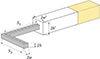 |
Figure 1. CAD design of a modelled λ/4-resonator. The design consists of three areas: a resonator (grey area), a baffle (white area) and a perfectly matched layer (yellow area). |
Dimensions of the modelled λ/4-resonators. The values of 2w′ and 2h′ are rounded to the nearest unit to increase readability.
For each of the 168 resonators, the length correction factor δ is calculated from the identified resonance frequency using equation (12):
 (12)
(12)
with c the sonic speed inside the resonator, equal to  .
.
3.2 Derivation of δ
Figure 2 shows δ in function of S1/L for all 168 resonators. When looking at Figure 2, several conclusions can be drawn. Firstly, it can be seen that δ≤0; the effective length of a folded resonator is always smaller than its centreline length. This implies that folding leads to an increase in resonance frequency, which is in line with earlier experimental findings [21]. Secondly, it can be seen that |δ| decreases when S1/L increases. This is expected, since δ must be zero (i.e. L′=L) when S1/L=1. Lastly, it can be seen that, for a fixed value of L, |δ| increases when 2w increases.
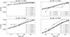 |
Figure 2. Relation between S1/L and δ for all 168 modelled resonators, grouped per value of 2w. (a) 2w=1 mm. (b) 2w=3 mm. (c) 2w=4 mm. (d) 2w=6 mm. |
Since δ∝2w and 1/δ∝S1/L, the following non-dimensional relationship can be set out [20, 37, 38]:
 (13)
(13)
Figure 3 shows the relation between the left and right side of equation (13)1 for all 168 resonators. When comparing Figures 3a–3f, it can be seen that the data points corresponding to L=0.2858 m do not follow the general trend. This is because the 1 Hz resolution of the numerical simulations is too coarse to get an accurate prediction of δ at very low frequencies. Hence, these 28 data points are excluded from further (regression) analyses. A bivariate regression analysis is now performed on the remaining 140 data points to derive the eventual expression for δ/(2w). Given the strong overlap between these points, a single regression line can be fit. This line is set to be a cubic polynomial, which has a general form given by a1x3+a2x2+a3x+a4. The coefficients of the polynomial are optimised using the least squares method (scipy.optimize.curve_fit), while meeting the following constraint: a4=−(a1+a2+a3). This constraint forces δ to be 0 when S1/L=1. Eventually, equation (14) is obtained:
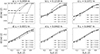 |
Figure 3. Relation between S1/L and δ/(2w) for all 168 resonators, grouped per value of L. (a) L=0.2858 m. (b) L=0.1319 m. (c) L=0.1072 m. (d) L=0.0572 m. (e) L=0.0463 m. (f) L=0.0407 m. |
 (14)
(14)
The coefficients in equation (14) are rounded to increase readability. The accuracy of equation (14) is assessed for the 140 resonators using a three-step approach:
-
The absorption coefficient of each resonator is calculated analytically using the formulas presented in Section 2 with L′=L (i.e. without any length correction) and its resonance frequency is determined;
-
The relative error between the numerical and analytical resonance frequency is calculated;
-
Equation (14) is integrated into the analytical model so that L′=L+δ and the two previous steps are repeated.
The results are shown in Figure 4. When looking at Figure 4, it can be seen that the accuracy of the analytical model drastically increases when equation (14) is applied: the maximum absolute value of the relative error drops from 6.3% to 0.4%, or in terms of frequency, from 134 Hz to 8 Hz. It is seen that the gain in accuracy is largest for the smallest value of L. This is expected, as the relative impact of δ on L′ increases when L decreases. It is also noticed that, for a fixed value of L, the absolute value of the relative error generally increases with 2w. This implies an additional dependence of δ on 2w, which is not yet accounted for in the current equation. As it is expected that accounting for this additional dependence will further increase the model accuracy, equation (13) is adapted to equation (15):
 (15)
(15)
with 2w0 a reference width [44]. In this paper, the reference width is set to 6 mm, the largest 2w-value in the data pool. The relation between S1/L and δ/(2w) for the 35 resonators with 2w=6 mm and between 2w/(2w0) and δ/(2w) for the 140 data points is shown in Figure 5. Since δ/(2w) is now function of two dimensionless ratios, two bivariate regression analyses are performed to derive the eventual expression for δ/(2w). Firstly, the relation between S1/L and δ/(2w) is analysed for the 35 6×5 mm2-resonators. Based on Figure 5a, this relation can be approximated by a cubic polynomial. The coefficients of this polynomial are again optimised using the least squares method (scipy.optimize.curve_fit), using the same constraint as when deriving equation (14). Since the fit is now based on 35 data points instead of 140, the coefficients of this cubic polynomial will be different compared with equation (14). Secondly, the relation between 2w/(2w0) and δ/(2w) is analysed for all 140 data points. Based on Figure 5b, this relation can be approximated by a quadratic polynomial, which has a general form given by b1x2+b2x+b3. The coefficients of this polynomial are also optimised using the least squares method (scipy.optimize.curve_fit), this time meeting the following constraint: b3=1−(b1+b2). This constraint forces the fit to be optimal when 2w=2w0. Eventually, equation (16) is obtained:
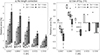 |
Figure 4. Overview of the relative error between the numerical and analytical resonance frequency for the 140 resonators, either or not applying equation (14). Each dot represents a different resonator. (a) No length correction. (b) Use of equation (14). |
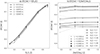 |
Figure 5. Relation (a) between S1/L and δ/(2w) for the 35 resonators with 2w=6 mm, and (b) between 2w/(2w0) and δ/(2w) for all 140 resonators. (a) δ/(2w)=f(S1/L). (b) δ/(2w)=f(2w/(2w0)). |
 (16)
(16)
with ς and υ representing S1/L and 2w/(2w0), respectively [44]. The coefficients in equation (16) are rounded to increase readability. The accuracy of equation (16) is compared with the accuracy of equation (14) and the results of this comparison are visualised in Figure 6. When Figure 6 is looked at, it can be seen that accounting for the additional dependence of δ on 2w has indeed further increased the model accuracy: the maximum absolute value of the relative error drops from 0.4% to 0.35%, or in terms of frequency, from 8 Hz to 5 Hz. Additionally, the relative error has become less dependent on the values of L and 2w as compared with using equation (14).
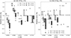 |
Figure 6. Overview of the relative error between the numerical and analytical predicted resonance frequency for the 140 resonators, applying either equation (14) or equation (16). Each dot represents a different resonator. (a) Use of equation (14). (b) Use of equation (16). |
3.3 Comparison with other length (correction) formulas
To support the earlier claim that the formula presented by Catapane G. et al. will not yield accurate results for resonators with separate 90° folds, said formula is applied to determine the resonance frequency of the remaining 140 data points. Since it now concerns λ/4-resonators with 90° folds instead of U-turns, this formula first has to be adapted, resulting in equation (17):
 (17)
(17)
Then, equation (17) is implemented into the analytical model and, for each resonator, the relative error between the numerical and analytical resonance frequency is calculated. The results are visualised in Figure 7. When Figures 6b and 7 are compared, several conclusions can be drawn. Firstly, it can be seen that the dependence of the relative error on both L and 2w is much larger for equation (17) than for equation (16). Secondly, based on the distance between the whiskers, it can be concluded that the accuracy of equation (17) is generally more dependent on S1/L as compared with equation (16). Lastly, it can be seen that equation (17) indeed yields significantly less accurate results than equation (16), especially at smaller centreline lengths. This was expected, since in equation (17), L′ solely depends on 2w, while in equation (16), L′ is function of both 2w and S1. The use of Pythagoras’ theorem is not included in this comparison since it is unclear which zigzag sound propagation path should be assumed.
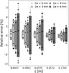 |
Figure 7. Relative error in predicted resonance frequency when applying equation (17). Each dot represents a different resonator. |
3.4 Verification of δ for other single-fold resonators
Given the data used to derive δ, equation (16) should be valid for any resonator that meets the following requirements: (i) 0.1319 m≥L≥0.0407 m, (ii) 2w≤6 mm, and (iii) one 90° fold with its centre at a distance between 0.1L and 0.9L from the resonator opening. In this section, the validity of δ is verified for 160 unique and arbitrary resonator geometries that meet these requirements. These resonators are divided into three sets:
-
Set A consists of resonators that have the same cross-section dimensions as those listed in Table 1, but have other values for L and S1/L;
-
Set B consists of resonators that have different cross-section dimensions than those listed in Table 1, but have the same values for L and S1/L;
-
Set C consists of resonators that have the same cross-section dimensions as the resonators in Set B and the same values for L and S1/L as the resonators in Set A.
An overview of the resonator geometries used for model verification is given in Table 2. Each resonator is modelled in COMSOL MultiPhysics® as described in Section 3.1 and the accuracy of equation (16) is determined as described in Section 3.2. The results are shown in Figure 8.
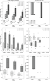 |
Figure 8. Overview of the relative error between the numerical and analytical predicted resonance frequency for the resonators in Set A (top), Set B (middle) and Set C (bottom), either or not applying equation (16). Each dot represents a different resonator. (a) No length correction. (b) Use of equation (16). |
An overview of the resonator geometries in Set A (top), Set B (middle) and Set C (bottom). The values of 2w′ and 2h′ are rounded to the nearest unit to increase readability.
When looking at Figure 8, it can be seen that applying equation (16) leads to an improved model accuracy. The maximum absolute value of the relative error when applying equation (16) is now 0.20%, or in terms of frequency, 4 Hz. As these values are in line with the error values in Section 3.2, it can be concluded that the use of equation (16) is justified within the proposed ranges for 2w, L and S1/L.
4 Experimental validation
Now that equation (16) is successfully verified, its use is also experimentally validated by means of impedance tube measurements on 3D printed samples.
An overview of the samples used for model validation is given in Table 3. To ensure sufficiently high absorption, each sample consists of either eight identical 3×3 mm2 or four identical 5×3 mm2 λ/4-resonators in parallel. The dimensions of the resonators fall within the validity range of equation (16) and are chosen so that the effect of folding should be clearly noticeable. All samples are printed with an Ultimaker S3 printer using the intent Engineering-profile [45]. As this profile is associated with a high dimensional accuracy, the dimensions of the printed resonators are expected to be close to the CAD dimensions, which should lead to representative experimental results. The samples are made out of Makerfill red PLA, as shown in Figure 9. The printer itself is placed in a climate-conditioned room to avoid additional temperature variability.
 |
Figure 9. Pictures of two 3D printed samples used for model validation. |
Once printed, each sample is mounted on an in-house impedance tube (∅=40 mm) to determine its maximum absorption coefficient and resonance frequency. The impedance tube test setup is illustrated in Figure 10. The measurements are performed according to the ISO 10534-2:1998 standard [46].
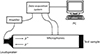 |
Figure 10. Sketch of the measurement set-up. |
4.1 Manufacturing inaccuracies in 3D printed parts
Due to manufacturing inaccuracies, the geometry of 3D printed resonators will be different from the CAD design, which might translate into an off-design performance. Since the aim of this section is to validate the accuracy of equation (16), it is important to know to which extent manufacturing inaccuracies contribute to the discrepancy between experimental and analytical results so that conclusive statements can be made with regard to the model accuracy. To this end, sample I (see Tab. 3) is printed four consecutive times using the exact same G-code file and without recalibrating the printer in between prints. The theoretical and experimental absorption curves of samples I(1) to I(4) are shown in Figure 11.
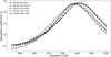 |
Figure 11. Analytical and experimental absorption curves of samples I(1) to I(4) [44]. |
When looking at Figure 11, it can be seen that the difference in maximum experimental absorption coefficient αmax (exp) between the four samples is limited, while the difference in experimental resonance frequency fR (exp) between the samples is significant. It can also be seen that the four experimental absorption curves deviate from the analytical result. The discrepancies in both αmax (exp) and fR (exp) between the samples can be attributed to manufacturing inaccuracies and tolerances.
More specifically, the discrepancies in αmax (exp) can be attributed to the non-ideality of the resonator cross-section, as shown in Figure 12: neither resonator has a perfectly rectangular cross-section, all resonators measure under 5 and 3 mm at their widest points and the rounding radius is not constant within and between samples, even though all resonators are printed with the same nozzle. These non-idealities will affect the visco-thermal losses that occur inside the resonator and, hence, the value of αmax (exp). There are also clear differences in surface quality between the four samples, which might also affect the absorption coefficient. The discrepancies in fR (exp) between the samples can be attributed to geometric tolerances in the Z-axis. Each resonator of the reference sample is designed with an outer length of 0.042 m, but since a Z-dimension of 42 mm requires a non-integer number of layers (279.7), the slicer software rounds the number of layers to the nearest integer value (280), which results in a targeted Z-dimension of 42.05 mm instead. However, the outer lengths of the printed resonators are found to vary between 41.9 mm and 42.25 mm, as shown in Table 4. Hence, it is assumed that L will also differ from its targeted value of 41 mm, resulting in an off-design resonance frequency.
 |
Figure 12. Microscopic images of the resonator cross-sections of the four reference samples, grouped per row. The scale of the microscopic images is 0.25 mm/division [44]. |
Outer lengths of the resonators of the reference samples, measured with the outer jaws of a digital caliper.
In sum, it can be stated that (i) there can be substantial differences in dimensional accuracy between 3D printed samples, even when the same printer settings are used and (ii) the influence of the overall print quality (i.e. manufacturing inaccuracies, tolerances and surface quality) on the acoustic performance of a λ/4-resonator cannot be neglected. Hence, it is suggested to use measured resonator dimensions as model input instead of CAD dimensions such that the shift in α and fR due to dimensional inaccuracies is already accounted for in the analytical model and the remaining error between model and experiments can mainly be attributed to model inaccuracies.
4.2 Repeatability of impedance tube measurements
Prior to the experimental validation, the repeatability of the impedance tube measurements was determined. To this end, a sample out of Table 3 was selected and repeatedly (re)mounted to the impedance tube. Each time, its absorption coefficient was measured and the resonance frequency of the sample was determined. In this work, sample G was selected since it has average values for L and S1/L. In total, eight test runs were performed and the repeatability of the test procedure was evaluated using the repeatability coefficient κ, which is defined as the value under which the absolute difference between two repeated measurements will lie with a 95% probability and can be calculated using equation (18):
 (18)
(18)
with σ2 the variance on the measured quantity [47]. In this work, the measured quantity is the resonance frequency and κ was found to be ≊4 Hz.
4.3 Accuracy of δ
To evaluate the accuracy of equation (16), impedance tube measurements are performed on all samples out of Table 3. Once a sample is tested, the test data is saved and the dimensions of each resonator of that sample are measured as follows:
-
The average cross-section dimensions
 and
and  of each resonator are determined using a microscope. It should be noted that the values of
  and
and  are assumed to be constant over depth, which might not be the case in reality.
 -
The actual centreline length
 of each resonator is measured using a digital caliper. For samples A–D,
  of each resonator is estimated out of the outer dimensions as the cross-section is too small to fit the depth rod of the caliper. For samples E–G, the resonators are cut open and direct depth measurements are performed.
Then, for each sample, four analytical absorption curves are calculated: α (C,−), α (C,δ), α (M,−), and α (M,δ). The letters “C” and “M” indicate whether the CAD or measured resonator dimensions were used as model input, while “–” and “δ” specify whether L′ in equation (2) equalled L or L+δ, respectively, with δ calculated using equation (16). The properties of air are calculated using the same ambient air temperature and pressure as measured during the tests. These four curves are then compared to the experimental results (α (exp)). An overview of the results for samples A–D and samples E–H is given in Figures 13 and 14, respectively.
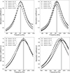 |
Figure 13. Experimental and analytical results for samples A to D. The grey area indicates the area in which the experimental resonance frequency is situated, taking into account the repeatability of the test procedure. |
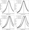 |
Figure 14. Experimental and analytical results for samples E to H. The grey area indicates the area in which the experimental resonance frequency is situated, taking into account the repeatability of the test procedure. |
The accuracy of equation (16) is now assessed in terms of the absolute error ψ as defined by equations (19)–(22):
 (19)
(19)
 (20)
(20)
 (21)
(21)
 (22)
(22)
An overview of the measured and calculated resonance frequencies and absolute errors for samples A to D and samples E to H is given in Tables 5 and 6, respectively. When looking at Tables 5 and 6, several conclusions can be drawn. Firstly, it can be concluded that, in general,  and
and  , which implies that using the measured resonator dimensions as model input indeed allows for a more accurate prediction of the resonance frequency compared with using the CAD dimensions. Secondly, when looking closer into the values of
  , it is seen that, on average,
  is larger for samples A to D than for samples E to H. This is attributed to L′ of the resonators of samples A to D being estimated instead of directly measured, but further research is needed to establish this conclusion. Lastly, it can be seen that implementing equation (16) does increase the accuracy of the model as |ψ(M,δ)|≤|ψ(M,−)| for each sample. The maximum value for |ψ(M,δ)| is 5 Hz, while the maximum value for |ψ(M,−)| is 49 Hz. When accounting for the repeatability of the test procedure, these values increase to 9 and 53 Hz, respectively.
5 Conclusions
In this paper, steps are taken towards the definition of a formula to calculate the effective length of a λ/4-resonator with separate 90° folds. More specifically, the effect of a 90° fold on the effective length of rectangle and slit-like λ/4-resonators is investigated numerically and a length correction factor δ is derived to account for this effect in the analytical model. It is found that δ is directly proportional to the resonator width and inversely proportional to the nearness of the fold to the resonator opening. The expression for δ is then verified numerically using COMSOL MultiPhysics® and validated experimentally by means of impedance tube measurements on 3D printed samples. Out of the experimental validation, it follows that δ grasps the effect of folding correctly and that the implementation of δ leads to a significant increase in the model accuracy: the maximum error between model and experiments drops from 49 Hz to 5 Hz. When the results of the experimental validation are studied more closely, it is noticed that using the measured resonator dimensions generally results in a higher model accuracy compared with using the CAD dimensions. Further steps include investigating (i) if and how δ can be applied to model rectangle and slit-like λ/4-resonators with multiple separate 90° folds, (ii) if and how δ can be applied to model rectangle and slit-like λ/4-resonators with U-turns (cf. labyrinth layout) and (iii) if the presented approach can also be applied to model λ/4-resonators with non-90° folds and λ/4-resonators with other cross-section shapes.
If the resonator is folded along 2h instead of 2w, the parameter 2w in equation (13) is replaced by 2h.
Funding
The research of F. De Bie (fellowship no. 1S17424N) is funded by a personal grant from the Research Foundation Flanders (FWO).
Conflicts of interest
The authors declare to have no known competing financial interests or personal relationships that could have influenced the work described in this paper.
Data availability statement
The data will be made available upon request.
Author contribution statement
Femke De Bie: Conceptualization, Formal analysis, Methodology, Software, Validation, Visualization, Writing – original draft, Writing – review & editing. Hervé Denayer: Conceptualization, Methodology, Supervision, Writing – review & editing. Elke Deckers: Conceptualization, Methodology, Supervision, Writing – review & editing.
References
- L. Jaouen: Propagation models assuming a motionless skeleton, https://apmr.matelys.com/PropagationModels/MotionlessSkeleton/ [Google Scholar]
- M.L. Munjal: Acoustics of Ducts and Mufflers with Application to Exhaust and Ventilation System Design. John Wiley & Sons, 1987 [Google Scholar]
- J.F. Allard, N. Atalla: Propagation of Sound in Porous Media: Modelling Sound Absorbing Materials, 2nd edition. Chichester, 2009 [CrossRef] [Google Scholar]
- L. Chul Hyung, H. Myeong Jae, P. Tae Won, K. Young Sik, S. Kyoung Duck: A comparative study on the transmission loss of helmholtz resonator and quarter, half, conical half-wave resonator using acoustic analysis model. International Journal of Mechanical Engineering and Robotics Research 9, 1 (2020) 153–157 [Google Scholar]
- C. Chen, D. Zhibo, H. Gengkai, Y. Jun: A low-frequency sound absorbing material with subwavelength thickness. Applied Physics Letters 110 (2017) 221903 [CrossRef] [Google Scholar]
- Y. Min, C. Shuyu, F. Caixing, S. Ping: Optimal sound-absorbing structures. Materials Horizons 4 (2017) 673–680 [CrossRef] [Google Scholar]
- W. Yutao, L. Qingxuan, H. Jin, F. Jiaming, C. Tianning: Deep-subwavelength broadband sound absorbing metasurface based on the update finger coiling-up method. Applied Acoustics 195 (2022) 108846 [CrossRef] [Google Scholar]
- Y. Zhu, K. Donda, F. Shiwang, C. Liyun, B. Assouar: Broadband ultra-thin acoustic metasurface absorber with coiled structure. Applied Physics Express 12, 11 (2019) 114002 [CrossRef] [Google Scholar]
- Y. Wang, H. Zhao, H. Yang, J. Zhong, D. Zhao, Z. Lu, J. Wen: A tunable sound-absorbing metamaterial based on coiled-up space. Journal of Applied Physics 123 (2018) 185109 [CrossRef] [Google Scholar]
- X. Lei, W. Gongxian, L. Gang, S. Jiahe, D. Zigiang, W. Shengtian: Optimization of hybrid microperforated panel and nonuniform space-coiling channels for broadband low-frequency sound absorption. Applied Acoustics 216 (2024) 109763 [CrossRef] [Google Scholar]
- W. Gongxian, L. Gang, X. Lei, Y. Xuewen: Low-frequency broadband absorber with coherent coupling based on perforated panel and space-coiling channels. Journal of Physics D: Applied Physics 56, 49 (2023) 495102 [CrossRef] [Google Scholar]
- W. Fei, X. Yong, Y. Dianlong, Z. Honggang, W. Yang, W. Jihong: Low-frequency sound absorption of hybrid absorber based on micro-perforated panel and coiled-up channels. Applied Physics Letters 114 (2019) 151901 [CrossRef] [Google Scholar]
- W. Yang, Z. Honggang, Z. Haibin, Z. Jie, W. Jihong: A space-coiled acoustic metamaterial with tunable low-frequency sound absorption. Europhysics Letters 120, 5 (2018) 54001 [Google Scholar]
- T. Zhang, F. Wu, C. Bai, K. An, J. Wang, B. Yang, D. Zhang: Acoustic metamaterial composed of zigzag channel and micro-perforated plate for enhanced low-frequency sound absorption. Journal of Vibration and Control 30, 13, 14 (2024) 2894–2903 [CrossRef] [Google Scholar]
- S. Ren, Y. Liu, W. Sun, H. Wang, Y. Lei, H. Wang, X. Zeng: Broadband low-frequency sound absorbing metastructures composed of impedance matching coiled-up cavity and porous materials. Applied Acoustics 200 (2022) 109061 [CrossRef] [Google Scholar]
- W. Yipu, W. Yonghua, W. Jinkai, Y. Huadong, Z. Chengchun, R. Luguan: Broadband low-frequency sound absorption by coiled-up space embedded in a porous layer. Applied Acoustics 182 (2021) 108226 [CrossRef] [Google Scholar]
- Y. Wang, H. Yuan, Y. Wang, J. Xu, H. Yu, C. Zhang, L. Ren: A study on ultra-thin and ultra-broadband acoustic performance of micro-perforated plate coupled with coiled-up space structure. Applied Acoustics 200 (2022) 109048 [CrossRef] [Google Scholar]
- L. Qinhao, D. Guoqing: A high-performance sound insulation component for filter capacitors based on coiled-up acoustic metamaterials. Physica Status Solidi A 219, 14 (2022) 2200125 [CrossRef] [Google Scholar]
- Z. Chi, H. Xinhua: Three-dimensional single-port labyrinthine acoustic metamaterial: perfect absorption with large bandwidth and tunability. Physical Review Applied 6 (2016) 064025 [CrossRef] [Google Scholar]
- G. Catapane, D. Magliacano, G. Petrone, A. Casaburo, F. Franco, S. De Rosa: Labyrinth resonator design for low-frequency acoustic meta-structures, in: International Conference on Wave Mechanics and Vibrations. Springer International Publishing, Cham, 2022, pp. 681–694 [Google Scholar]
- Z. Zhang, F. De Bie, H. Denayer, C. Claeys, W. Desmet, E. Deckers: Optimized metamaterial using quarter-wavelength resonators for broadband acoustic absorption, in: Proceedings of DAGA2021, 2021, pp. 101–104 [Google Scholar]
- A.C. De Sousa, E. Deckers, C. Claeys, W. Desmet: On the assembly of archimedean spiral cavities for sound absorption applications: design, optimization and experimental validation. Mechanical Systems and Signal Processing 147 (2021) 107102 [CrossRef] [Google Scholar]
- G. Jingwen, Z. Xin, F. Yi, Q. Renhao: An extremely-thin acoustic metasurface for low-frequency sound attenuation with a tunable absorption bandwidth. International Journal of Mechanical Sciences 213 (2022) 106872 [CrossRef] [Google Scholar]
- H. Mingming, W. Junxiang, Y. Skaokun, W. Jiu Hui, M. Fuyin: Expanding the strong absorption band by impedance matched mosquito-coil-like acoustic metamaterials. Review of Scientific Instruments 91 (2020) 025102 [CrossRef] [PubMed] [Google Scholar]
- I. Prasetiyo, K. Anwar, F. Brahmana, K. Sakagami: Development of stackable subwavelength sound absorber based on coiled-up system. Applied Acoustics 195 (2022) 108842 [CrossRef] [Google Scholar]
- S. Gang Yong, C. Qiang, H. Bei, D. Hui Yuan, C. Tie Jun: Broadband fractal acoustic metamaterials for low-frequency sound attenuation. Applied Physics Letters 109 (2016) 131901 [CrossRef] [Google Scholar]
- G. Comandini, C. Khodr, V.P. Ting, M. Azarpeyvand, F. Scarpa: Sound absorption in Hilbert fractal and coiled acoustic metamaterials. Applied Physics Letters 120 (2022) 061902 [CrossRef] [Google Scholar]
- C. Hongyu, L. Chengtao, H. Haoming: Research on low-frequency noise control based on fractal coiled acoustic metamaterials. Shock and Vibration 2022 (2022) 2083563 [Google Scholar]
- Y. Lin, Z. Ruoxi, W. Xiaoxiao, W. Shuxia: Near-perfect low-frequency sound absorption in subwavelength H-fractal metamaterials. Applied Physics Express 16, 8 (2023) 087001 [CrossRef] [Google Scholar]
- M. Boccaccio, F. Bucciarelli, G.P.M. Fierro, M. Meo: Microperforated Panel and deep subwavelength Achimedean-inspired spiral cavites for multi-tonal and broadband sound absorption. Applied Acoustics 176 (2021) 107901 [CrossRef] [Google Scholar]
- M. Boccaccio, G.P.M. Fierro, F. Bucciarelli, M. Meo: Multi-tonal subwavelength metamaterial for absorption and amplification of acoustic and untrasonic waves. Engineering Research Express 3, 2 (2021) 025024 [CrossRef] [Google Scholar]
- L. Qiang, D. Ruizhi, M. Dongxing, W. Xu, L. Yong: A compact broadband absorber based on helical metasurfaces. International Journal of Mechanical Sciences 254 (2023) 108425 [CrossRef] [Google Scholar]
- G. Nansha, H. Hong: Sound absorption characteristic of micro-helix metamaterial by 3D printing. Theoretical and Applied Mechanics Letters 8, 2 (2018) 63–67 [CrossRef] [Google Scholar]
- S.H. Xie, X. Fang, P.Q. Li, S. Huang, Y.G. Peng, Y.X. Shen, Y. Li, X.F. Zhu: Tunable double-band perfect absorbers via acoustic metasurfaces with nesting helical tracks. Chinese Physics Letters 37, 5 (2020) 054301 [CrossRef] [Google Scholar]
- L. Zixian, L. Jensen: Extreme acoustic metamaterial by coiling up space. Physical Review Letters 108, 11 (2012) 114301 [CrossRef] [PubMed] [Google Scholar]
- R. Ghaffarivardavagh, J. Nikolajczyk, R. Glynn Holt, S. Anderson, Z. Xin: Horn-like space-coiling metamaterials toward simultaneous phase and amplitude modulation. Nature Communications 9 (2018) 1349 [CrossRef] [PubMed] [Google Scholar]
- F. De Bie, H. Denayer, C. Claeys, E. Deckers: Quarter-wavelength acoustic metamaterials: the effect of folding on the resonance frequency, in: Proceedings of ISMA2022-USD2022, 2022, pp. 3054–3065 [Google Scholar]
- T. Cambonie, F. Mbailassem, E. Gourdon: Bending a quarter wavelength resonator: curvature effects on sound absorption properties. Applied Acoustics 131 (2018) 87–102 [CrossRef] [Google Scholar]
- B.E. Anderson: Understanding radiation impedance through animations. Proceedings of Meetings on Acoustics 33 (2020) 025003 [Google Scholar]
- L. Jaouen, F. Chevilotte: Length correction of 2D discontinuities or performations at large wavelengths and for lineair acoustics. Acta Acustica united with Acustica 104, 2 (2018) 243–250 [CrossRef] [Google Scholar]
- D.E. Weston: The theory of the propagation of plane sound waves in tubes. Proceedings of the Physical Society. Section B 66, 8 (1953) 695–709 [CrossRef] [Google Scholar]
- M.R. Stinson: The propagation of plane sound waves in narrow and wide circular tubes, and generalization to uniform tubes of arbitrary cross-sectional shape. The Journal of the Acoustical Society of America 89 (1991) 550–558 [CrossRef] [Google Scholar]
- T.G. Zieliński, F. Chevilotte, E. Deckers: Sound absorption of plates with micro-slits backed with air cavities: analytical estimations, numerical calculations and experimental validations. Applied Acoustics 146 (2019) 261–279 [CrossRef] [Google Scholar]
- F. De Bie, H. Denayer, C. Claeys, E. Deckers: Experimental validation of the length correction factor for folded quarter-wavelength resonators, in: Proceedings of Forum Acusticum, 2023, pp. 1969–1976 [Google Scholar]
- Intent profiles in UltiMaker Cura, https://support.makerbot.com/s/article/1667411132905 [Google Scholar]
- ISO 10534-2 standard: Acoustics – determination of acoustic properties in impedance tubes – part 2: two-microphone technique for normal sound absorption coefficient and normal surface impedance, 1998 [Google Scholar]
- ISO 5725-6 standard: Accuracy (trueness and precision) of measurement methods and results – part 6: use in practice of accuracy values, 1994 [Google Scholar]
Cite this article as: De Bie F. Denayer H. & Deckers E. 2025. Derivation, verification and validation of a length correction factor for folded quarter-wavelength resonators. Acta Acustica, 9, 38. https://doi.org/10.1051/aacus/2025022.
All Tables
Dimensions of the modelled λ/4-resonators. The values of 2w′ and 2h′ are rounded to the nearest unit to increase readability.
An overview of the resonator geometries in Set A (top), Set B (middle) and Set C (bottom). The values of 2w′ and 2h′ are rounded to the nearest unit to increase readability.
Outer lengths of the resonators of the reference samples, measured with the outer jaws of a digital caliper.
All Figures
|
Figure 1. CAD design of a modelled λ/4-resonator. The design consists of three areas: a resonator (grey area), a baffle (white area) and a perfectly matched layer (yellow area). |
| In the text | |
|
Figure 2. Relation between S1/L and δ for all 168 modelled resonators, grouped per value of 2w. (a) 2w=1 mm. (b) 2w=3 mm. (c) 2w=4 mm. (d) 2w=6 mm. |
| In the text | |
|
Figure 3. Relation between S1/L and δ/(2w) for all 168 resonators, grouped per value of L. (a) L=0.2858 m. (b) L=0.1319 m. (c) L=0.1072 m. (d) L=0.0572 m. (e) L=0.0463 m. (f) L=0.0407 m. |
| In the text | |
|
Figure 4. Overview of the relative error between the numerical and analytical resonance frequency for the 140 resonators, either or not applying equation (14). Each dot represents a different resonator. (a) No length correction. (b) Use of equation (14). |
| In the text | |
|
Figure 5. Relation (a) between S1/L and δ/(2w) for the 35 resonators with 2w=6 mm, and (b) between 2w/(2w0) and δ/(2w) for all 140 resonators. (a) δ/(2w)=f(S1/L). (b) δ/(2w)=f(2w/(2w0)). |
| In the text | |
|
Figure 6. Overview of the relative error between the numerical and analytical predicted resonance frequency for the 140 resonators, applying either equation (14) or equation (16). Each dot represents a different resonator. (a) Use of equation (14). (b) Use of equation (16). |
| In the text | |
|
Figure 7. Relative error in predicted resonance frequency when applying equation (17). Each dot represents a different resonator. |
| In the text | |
|
Figure 8. Overview of the relative error between the numerical and analytical predicted resonance frequency for the resonators in Set A (top), Set B (middle) and Set C (bottom), either or not applying equation (16). Each dot represents a different resonator. (a) No length correction. (b) Use of equation (16). |
| In the text | |
|
Figure 9. Pictures of two 3D printed samples used for model validation. |
| In the text | |
|
Figure 10. Sketch of the measurement set-up. |
| In the text | |
|
Figure 11. Analytical and experimental absorption curves of samples I(1) to I(4) [44]. |
| In the text | |
|
Figure 12. Microscopic images of the resonator cross-sections of the four reference samples, grouped per row. The scale of the microscopic images is 0.25 mm/division [44]. |
| In the text | |
|
Figure 13. Experimental and analytical results for samples A to D. The grey area indicates the area in which the experimental resonance frequency is situated, taking into account the repeatability of the test procedure. |
| In the text | |
|
Figure 14. Experimental and analytical results for samples E to H. The grey area indicates the area in which the experimental resonance frequency is situated, taking into account the repeatability of the test procedure. |
| In the text | |
Current usage metrics show cumulative count of Article Views (full-text article views including HTML views, PDF and ePub downloads, according to the available data) and Abstracts Views on Vision4Press platform.
Data correspond to usage on the plateform after 2015. The current usage metrics is available 48-96 hours after online publication and is updated daily on week days.
Initial download of the metrics may take a while.