| Issue |
Acta Acust.
Volume 9, 2025
|
|
|---|---|---|
| Article Number | 60 | |
| Number of page(s) | 11 | |
| Section | Hearing, Audiology and Psychoacoustics | |
| DOI | https://doi.org/10.1051/aacus/2025048 | |
| Published online | 17 October 2025 | |
Scientific Article
Directional sharpness perception under different listening conditions
1
Department of Engineering Acoustics, Technische Universität Berlin, Einsteinufer 25, 10587, Berlin, Germany
2
Audio Communication Group, Technische Universität Berlin, Einsteinufer 17c, 10587, Berlin, Germany
* Corresponding author: This email address is being protected from spambots. You need JavaScript enabled to view it.
Received:
14
April
2025
Accepted:
3
September
2025
Abstract
The assessment of sounds using psychoacoustic parameters is important in many areas. For the binaural case, it is not sufficiently clear how the characteristics of both ear signals have to be combined so that they best reflect the binaural percept. In the case of the auditory sensation of sharpness, this is particularly unclear due to limited empirical data on the perception of sharpness in dichotic listening conditions. To expand the empirical database and allow discussion on calculation methods for binaural sharpness and the derivation of representative metrics reflecting the binaural percept, two listening experiments were designed and conducted. The participants evaluated a series of signals for their sharpness, which were presented as real sound sources in an anechoic chamber via loudspeakers and as virtual sound sources via headphones from different sound source positions in the horizontal plane. Paired comparison and rating scale methods have been used to collect the data. Both experiments on sharpness revealed a tendency towards decreasing sharpness perception across all lateral positions. In contrast to maximum sharpness values of the ipsilateral side, arithmetic and quadratic averaging (mean and RMS values) of sharpness calculated according to the Aures method reflected the listening test results well and appear to be promising approaches for determining a binaural single value for most of the considered signals. Monaural signals and signals with several sound sources showed particular abnormalities in the listening test, some of which cannot be explained well.
Key words: Binaural sharpness / Binaural psychoacoustic parameters / Psychoacoustic sharpness / Directional sharpness perception / Sharpness perception under dichotic listening conditions
© The Author(s), Published by EDP Sciences, 2025
 This is an Open Access article distributed under the terms of the Creative Commons Attribution License (https://creativecommons.org/licenses/by/4.0), which permits unrestricted use, distribution, and reproduction in any medium, provided the original work is properly cited.
1 Introduction
The importance of understanding binaural signal processing is undisputed, particularly as it relates to auditory sensations and sound perceptions in complex listening environments. Real-world listening situations usually involve spatially distributed sound sources, leading to dichotic listening conditions in which the signals differ at both ears. While binaural loudness has been extensively empirically researched [1–4] leading to several models, incorporated also in ISO loudness standards[5, 6], the perception of other psychoacoustic parameters under dichotic listening conditions, such as sharpness, roughness or fluctuation strength, remains less explored. The increasing use of artificial head measurement systems raises the question of how parameter estimates for the left and right ears should be combined to derive representative single values for dichotic conditions in binaural measurements. To suggest guidelines, it is necessary to understand how auditory sensations develop in dichotic listening situations. In two laboratory studies, the effect of different sound source positions in the horizontal plane on the perception of sharpness was investigated under two different listening conditions: (1) in an anechoic chamber using a setup of spatially distributed loudspeakers and (2) with virtual sound sources rendered with non-individual head-related transfer functions (HRTFs), and presented over headphones. With the help of paired comparison and rating scale methods data was collected and discussed with respect to strategies to derive representative single values for binaural sharpness sensations. This article extends our previous investigation [7] by (i) a comparison of sharpness ratings for virtual sources to previously unpublished sharpness ratings for real sources and (ii) a more detailed analysis of the results. This allows to additionally investigate if sharpness perception can be studied using non-individual virtual sound sources, which are easier to realise and control inpractice.
1.1 Monaural sharpness
Psychoacoustic sharpness is a measure of timbre, defined by the spectral centroid of a signal. It increases with the presence of high-frequency components and is primarily determined by the spectral envelope. Sharpness is generally calculated from the sum of the weighted specific loudness values across all critical bands (see [8]) where the weighting factor increases progressively from around 15 Bark (corresponding to 2700 Hz) onwards. The unit of sharpness is “acum", where 1 acum is defined as the sharpness elicited by a narrowband noise centered at 1 kHz at 60 dB (SPL). Although sharpness can be perceived independently of the loudness of a sound event, loudness does exert a small influence [8, 9].
Currently, three methods for calculating (monaural) sharpness are established: von Bismarck [10], Aures [11], and DIN 45692 [12]. They all differ in the weightings of the specific loudness levels for determining the spectral center of gravity. While Aures’ method takes into account the influence of total loudness on sharpness within the weighting function, the influence of total loudness is neglected in the other two methods. At least in a few studies, the representative value for perceived time-variant sound episodes has been investigated for the sensation of sharpness, indicating that time-average based metrics better reflect experimental data than percentile values as used for overall loudness [13].
1.2 Binaural sharpness
Analogous to directional loudness, directional sharpness perception is shaped by two distinguishable underlying processes. The first is the physical transmission of sound from the source to the eardrums, which can be described by head-related transfer functions (HRTFs). In a second psychophysical process, the direction-dependent signals at both eardrums are combined into a binaural percept [3, 14].
The left and right ear HRTFs are similar for sources in the median plane [15] but the similarity decreases as a source moves away from the median plane. Most notably, the high frequency energy increases at the ipsilateral ear and decreases at the contralateral (shadowed) ear as the source moves from the median plane to a more lateral position. For sources to the side of the listener this results in interaural level differences of approximately 5–10 dB below 3 kHz and more than 20 dB for frequencies above 3 kHz [16]. As HRTFs are well understood and their effects are already taken into account when using artificial head measurement systems, the remaining question is how to combine the sharpness values of both ear signals to best reflect the binaural percept.
While the binaural perception of loudness [1–4] or to a lesser extent roughness [17] have already been subject to past studies, binaural sharpness perception appears still largely unexplored. Nonetheless there have been made some proposals for the calculation of a single value for binaural listening which all are based on the assumption of a similar processing to that of binaural loudness.
Klemenz and Fels proposed a simple arithmetic average of the left and right channel for binaural sharpness [18]. Segura-Garcia et al. [19] introduced a binaural sharpness model purportedly based on Moore and Glasberg’s binaural loudness model [20]. In this theoretically derived approach, sharpness is first calculated for both channels (left and right) according to Fastl and Zwicker [8], and then summed with weighting based on the inhibition factor from Moore and Glasberg’s model for diotic loudness perception. The model suggests that binaural sharpness, like binaural loudness, involves a form of binaural summation. In contrast to it, in the ISO/TS 12913-2 [21] and ISO/TS 12913-3 [22] standards, which define the requirements for conducting soundscape studies, a different parameter is proposed, the maximum sharpness value of both ear signals. However, there is no empirical evidence for the binaural sharpness sensation regarding the adequacy of a maximum value compared to an average of both ear signals or any other calculation of a value reflecting binaural sharpness sensations.
As any binaural model needs to be based on solid empirical data, two listening experiments were designed and conducted varying binaural listening conditions.
2 Method
Based on two experiments the effects of lateral sound incidence angles in the horizontal plane on sharpness perception were investigated. While the first experiment was carried out in an anechoic chamber using a loudspeaker setup, virtual sound sources were presented via headphones in an audiometry cabin in the second experiment.
2.1 Paired comparison
Series of paired comparison tests were carried out in both listening experiments. In these, the participants were asked to choose one of two consecutive stimulus signals from different (virtual) directions that they perceived as sharper. As the participants had to choose a signal and there was no “equal" answer, a forced choice was required. In each paired comparison test, the participants were presented with all possible combinations of discrete (virtual) spatial positions of a signal in one half-space (0°–180° in the left or right space) for evaluation. Each position was presented against each other (excluding itself) only once (e.g., 0° vs. 30° or 30° vs. 0°). For n different sound source positions, the number of pairs then equaled n(n − 1)/2. The order in which the pairs and the positions within each pair were presented was randomized and it was not possible to change the selection after a response had been given. Detailed descriptions of the stimuli and presented pairs for each experiment are provided in Sections 2.3 and 2.4.
2.2 Rating scale
In order to obtain additional data using an alternative method, the rating scale method was implemented in the second experiment. A unipolar rating scale ranging from 0 (not at all) to 10 (extremely) was chosen. In order not to further increase the difficulty of the listening experiment and to be able to evaluate additional signals, the number of virtual sound source positions was reduced to three: 0°, 60°, and 135° (or −0°, −60°, and −135° in the left half-space). In addition to the signals from the paired comparison tests, additional signals were included in the tests using the rating scale, so that a total of 22 signals had to be judged. The order of signal presentation was randomized before each run. Each signal was presented only once and it was not possible to change the selection after logging an answer.
2.3 Experiment I
2.3.1 Participants
A total of 24 participants aged between 18 and 62 took part in the first experiment. The majority of the participants were aged 25–34. All participants stated that they had no hearing impairments.
2.3.2 Stimuli
Three different signals were used in the first experiment: (1) A white noise was generated in MATLAB using AKTools [23], with an upper cut-off frequency of 22 kHz. (2) A recording of a vacuum cleaner was taken from the Freesound.org library [24]. (3) As a natural sound, the recording of a bird chirping from the IADS-2 database [25] was used. It differed from the other time-invariant signal through its impulsiveness. While the first two signals were 5 s long, the bird chirping was around 6 seconds. The playback level of the signals at the listener position was set to 58 dB(A). Spectrograms of the three signals are shown in Figure 1.
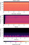 |
Figure 1 Spectrograms (window: Hanning; window length: 1024; window overlap: 50%) of the three signals used in the first experiment (anechoic chamber). |
2.3.3 Apparatus
The listening experiment was carried out in the anechoic chamber of the Technische Universität Berlin with a cut-off frequency of 63 Hz. Seven Neumann KH120A loudspeakers were arranged around the listener position at a distance of 3 m ± 1 cm in 30 ° ±0.3° steps from the front over the left side to the back. All loudspeakers were aligned in the direction of the listener position. The chair was aligned in the viewing direction of the 0° position, so that the ears were parallel to the 90° direction. A neck support attached to the chair minimized slippage of the ear position as shown in Figure 2. The acoustic center of the loudspeakers (between the tweeter and woofer drivers) was located 1.4 m ± 1 cm above the grille of the anechoic chamber at ear level of the participants. Stimuli playback, randomization as well as answer collection was handled by an App designed in the MATLAB App Designer specifically for this listening experiment. It run on a laptop that was placed on a loudspeaker stand about 20 cm in front of the listener chair. The signals were fed from the laptop via an RME Fireface UC – USB audio interface. To minimize influences such as room reflections or reflections caused by the anechoic chamber’s support grid or the laptop, as well as influences introduced by the loudspeaker playback itself, an equalization of the individual loudspeakers was performed at signal level. The frequency response of each loudspeaker was measured at a total of seven positions at and around the listener position using a 1.5-second long sweep signal. The measurements for each loudspeaker were then averaged across all positions and smoothed to one-sixth octave.
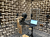 |
Figure 2 Full anechoic chamber used for experiment I with the listening position (where the artificial head is mounted) located in the center of the loudspeaker array. |
2.3.4 Experimental procedure
Prior to the experiment the participants had to generate an individual code for anonymisation and then were instructed on the task. Two joint practice runs were conducted together with the experimenter to familiarize the participants with the user interface and experimental procedure before the actual experiment began in isolation. Four paired comparison blocks were run on sharpness, one of which was a repeated run to assess retest reliability. The blocks were run in the following order: (1) white noise, (2) vacuum cleaner, (3) vacuum cleaner (retest), (4) birds. Before the first sharpness block on white noise and between the second block and the retest block with the vacuum cleaner stimulus, two other blocks investigating binaural loudness perception were carried out, the data from which will not be considered here. After completing three out of the total six experimental blocks, participants were given the opportunity to take a break, leave the anechoic chamber, and resume the experiment at their own will. Since seven sound source positions in the left half-space of the auditory space were chosen for this experiment (0°, 30°, 60°, 90°, 120°, 150°, 180°), each paired comparison block consisted of 21 pairs. For safety reasons, the experimenter monitored participants using a camera installed in the room from the outside of the anechoic chamber. After the experiment, the participants had to fill a questionnaire.
2.4 Experiment II
2.4.1 Participants
A total of 33 participants completed the listening test. Of these, the median age was 27 years (SD = 7.4) and the majority of participants were between 25 and 34 years old. Nine people stated female gender and 24 male. Twenty two of the 33 participants considered their hearing to be trained. Nine of the participants stated that they had expert knowledge of psychoacoustic parameters. More than half (n = 18) of the participants had no prior experience with listening experiments. Four people stated that they had “little" listening experiment experience, while eight had “some" and three “a lot". All participants stated that they had no hearing impairments.
2.4.2 Stimuli
The majority of signals for the second experiment were synthetic and generated in Python. Additionally recorded (real-world) signals from the Freesound.org [24] library were used, like in the first experiment. One signal from the first experiment, the bird chirping, was reused. All signals were generated monotic or reduced to a single channel, and then adjusted to an equal loudness according to ITU-R BS.1770 [26] prior to auralization. Virtual sources were rendered using head-related transfer functions for neutral head orientation from the FABIAN head-and-torso simulator database [27]. The headphone compensation filter for the used headphones (Sennheiser HD 800 S) from the FABIAN HRTF data base was convolved with the signals.
In the three paired comparison blocks the signals used were: (1) A sharp noise, generated from a white noise that was processed using a first-order Butterworth high-pass filter with a cut-off frequency of 2 kHz. One monaural signal without the sound averted ear channel was generated additionally for the 60° position. (2) The bird chirping from the first experiment. (3) A signal containing two sound sources was rendered: a narrowband noise, with a bandwidth corresponding to the critical band 19 (CB19), was consistently positioned at −90° in all auralizations, while the sharp noise was auralized at the usual positions on the other side.
For the rating scale block, the three signals where reused and four further ones were added: (1) A narrowband noise with a bandwidth of critical band 12 (CB12), (2) a flute playing a sequence of notes ascending in pitch, (3) pink noise band-pass filtered between 100 Hz and 10 kHz, and (4) the recording of the hissing pressure drop of a pressure cooker. Most signals were 4 s long, some recordings (signals “birds" and “flute") were left at their original length of around 6 s. The signals of the second experiment are shown as spectrograms in Figure 3 (excluding “birds", see Fig. 1).
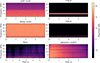 |
Figure 3 Spectrograms (window: Hanning; window length: 1024; window overlap: 50%) of the single channel signals (excluding “birds", see Fig. 1) used in the second experiment (audiometry cabin) prior to auralization. |
All signals used in experiment II were additionallyrendered without the headphone compensation filter. In the Artemis Suite software by HEAD acoustics, sound pressure levels were normalized to the measured levels from the pretest. Subsequently, sharpness was calculated for all signals and both channels, following DIN 45692 [12] and the method by Aures [11]. In both cases additionally the arithmetic and quadratic means (mean and RMS) of the sharpness of the two channels were calculated for each sound source position. The calculations are presented alongside the experimental results for each signal (see Sect. 3).
2.4.3 Apparatus
The listening experiment took place in an audiometry cabin at the Technische Universität Berlin. From the audiometry cabin, the participants were able to control the test application running on a laptop outside the booth using a mouse and keyboard. The test application was custom-developed in Python. A Sennheiser HD 800 S headphone was used and powered by an RME Audio Fireface UCX II. A photograph of the apparatus is provided in Figure 4. The playback level was set to the initially defined test level of approximately 68 dB(SPL) for the “pink noise" signal presented from the 0° position. This was measured in the pre-test using a HEAD acoustics artificial head HMS III. A background noise level of 26 dB(A) was recorded in the audiometry cabin using the sound level meter NTI Audio XL2.
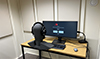 |
Figure 4 Audiometry cabin for the execution of experiment II and artificial head measurement system to adjust the playback level. |
2.4.4 Experimental procedure
After being welcomed, the participants first completed a questionnaire and generated an individual participant code for anonymization purposes. They were then instructed regarding the tasks to be performed. A total of four experimental blocks on sharpness were conducted in the following order: (1) paired comparisons for “sharp noise", including one specific pair with a monaural – binaural comparison, (2) paired comparisons for “birds", (3) paired comparisons for “CB19 sharp noise", and (4) rating scale judgments on all signals. The number of sound source positions in one half-space (left or right) in the horizontal plane was reduced to six in this experiment, following the methodology of Sivonen and Ellermeier[2–4]: 0°, 30°, 60°, 90°, 135°, and 180°. Consequently, the number of judgments per paired comparison block was 15 or 16 (including the additional monaural signal pair). The half-space (right or left) was alternated after each block and rotated after each participant to ensure that participants did not consistently hear from one side throughout the entire experiment, while also guaranteeing that both half-spaces were presented equally often across all blocks and participants. For the analysis, data from both sides were combined, assuming binaural symmetry in hearing. As in the first experiment, other psychoacoustic dimensions were assessed in this listening test as well. Prior to the four sharpness blocks, one block on loudness and four on roughness were conducted. The data from these will not be considered here.
3 Results
3.1 Experiment I
In paired comparisons, each participant provides a judgment regarding which signal is perceived as sharper for every possible combination of signals. These judgments, summed across all participants and divided by the total number of participants, yield the relative frequency with which each signal is chosen over every other (excluding itself). This information is typically represented in a dominance matrix. Averaging the relative frequencies of a stimulus as being perceived as sharper over others yields the averaged frequency with which a stimulus dominated other stimuli, here named as the “averaged win rate". From this, an ordinal scale ranking can be derived, which theoretically allows for inferences about stimulus intensities [28]. The ranking can be considered valid, when weak stochastic transitivity (WST) is fulfilled [29, 30]. All four paired comparison blocks showed no violations of WST. Results in Figure 5 show that for the white noise signal, the 0° position dominated over all other lateral positions in the paired comparison tests. Because the 30° position dominated even more clearly (80% win rate) over some positions (60°, 90°, 180°) its averaged win rate is only slightly behind the 0° position. The consistency coefficients ζ [31] of the paired comparison blocks, averaged across all participants, can be found in Table 1.
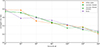 |
Figure 5 Results of the first experiment (anechoic chamber) showing the averaged win rate in the paired comparison tests per signal for the different spatial positions. |
The block with the vacuum cleaner recording yielded a clearer image of a dropping dominance over all lateral positions than the white noise block due to its consistently dropping win rate over all positions. In the retest block with the same signal (vacuum cleaner), the results were not as clear and a slight uncertainty appeared, as the 150° position was able to dominate over the 120° position. For the “birds" signal, although the dominance dropped noticeably from 0° to 30°, a subtle increase was observed to 60°, followed by a continuous decline across the remaining positions. Although differences were observed across individual positions, all signals followed the same overall trend of decreasing dominance with increasing lateral sound source position. As shown in the table, the consistency coefficient averaged across all participants was only ever just ζ ≥ 0.5 in all block. Since the number of participants in the first experiment was also not that high, the usual criteria for excluding participants with ζ < 0.6 [31] was not applied here.
3.2 Experiment II
3.2.1 Paired comparison
In the analysis of the paired comparison data from the second experiment, participants with consistency coefficients ζ < 0.6 were excluded according to common practice [31]. The cumulative data matrices of all three blocks showed no violations of WST, “sharp noise" and “CB19 sharp noise" even held moderate stochastic transitivity (MST), while “birds" showed 1 out of 20 possible violations. The averaged win rates over all sound source positions for the three stimulus signals presented in the paired comparison tests, together with their calculated and averaged sharpness according to the Aures method and DIN 45692, are shown in Figure 6.
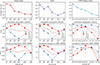 |
Figure 6 Results of the second experiment (audiometry cabin) showing the averaged win rate in the paired comparison tests for the signals “sharp noise", “birds", and “CB19 sharp noise" for the considered spatial positions (top), the results of sharpness method according to Aures [11] (middle) and the results of sharpness method according to DIN 45692 [12] (bottom). |
In the paired comparison test for the “sharp noise" signal, a continuous decrease in dominance was observed with increasing lateral sound incidence angle. The 180° position was only able to outperform the 135° position in 52% of the cases in direct comparison, which did not affect the overall dominance ranking of the sound source position. For the signal “birds", apart from the 0° position, the 60° position was particularly dominant, outperforming all other positions except for the 0° position in direct comparisons. A clear decrease in dominance across the lateral positions was not observed.
In contrast, for the signal “CB19 sharp noise" with two virtual sound sources, such a decrease in dominance across all positions was observed again. The number of remaining participants (N) and the averaged consistency coefficient (ζ) across all participants of the three paired comparison tests of the second experiment are listed in Table 2.
Number of remaining participants N and averaged consistency coefficient ζ of the paired comparison tests in the second experiment without participants with a consistency coefficient ζ < 0.6.
3.2.2 Rating scale
The results of all participants were included in the evaluation of the rating scale block and are shown in Figure 7 as mean values with 95% confidence intervals and rating densities for all included sound source positions for each signal. Visible differences in sharpness ratings between different sound source positions of a signal almost always result from decreased sharpness ratings for the more laterally displaced position.
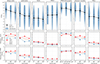 |
Figure 7 Results of the second experiment (audiometry cabin) showing the rating scale assessment results for all signals as mean values with 95% confidence intervals and rating distribution (top), the results of sharpness method according to Aures [11] (middle) and the results of sharpness method according to DIN 45692 [12] (bottom). |
The ratings for the three positions of each signal were first tested for differences using a repeated measures ANOVA. Dependent t-tests for paired data with Bonferroni correction were performed as post-hoc tests and Cohen’s d was calculated to determine effect sizes. The ANOVA analysis revealed significant differences in the ratings of the virtual sound source positions for the signals “sharp noise" (F(2, 64)=6.91; p < 0.01**), “pink noise" (F(2, 64)=4.96; p < 0.05*), “pressure cooker" (F(2, 64)=3.60; p < 0.05*), and “birds" (F(2, 64)=3.17; p < 0.05*). For the two signals “sharp noise" and “pink noise", differences in sharpness ratings occurred between the 0° and 135° sound source positions. For “sharp noise" signal, the t-test for the difference between the 0° and 135° positions even indicated a highly significant effect (p < 0.001***). For the “pink noise" signal, the t-test also provided a significant p-value for the decrease in sharpness ratings from 0° to 60° (p < 0.05*). The crucial difference for the “pressure cooker" signal occurred between the 60° and 135° position. For the “birds" signal, the effect detected by the ANOVA could not withstand the Bonferroni post hoc corrections and no significant difference in sharpness ratings between two sound incidence angles was found. The effect sizes according to Cohen’s d were in the small to medium range and are shown in Table 3. According to Cohen, a small effect is present at a d ≥ 0.2, a medium effect at d ≥ 0.5 and a large effect at d ≥ 0.8 [32].
Effect sizes (Cohen’s d) for the rating scale results. Bold indicates at least a small effect (|d|≥0.20). Asterisks denote Bonferroni-corrected t-test significance: * p < .05, ** p < .01, *** p < .001.
3.3 Monaural signals
In a direct comparison (paired comparison), the monaural “sharp noise" signal (60°) without the contralateral channel was rated as sharper 18 times, slightly more often than the same signal presented binaurally (15 times). In the rating scale, the mean scores were 7.24 (monaural)and 6.81 (binaural). However, a t-test did not confirm this difference in means as significant (p = 0.14).
4 Discussion
4.1 Directional sharpness perception
The paired comparison tests of both listening experiments yielded similar results. In both the anechoic chamber and the headphone-based experiment with virtual sound sources, dominance generally decreased with increasing lateral sound incidence angle in the horizontal plane towards more posterior positions, with only a few exceptions. For the signal “birds", used in both experiments, a slightly increased dominance at the 60° position was observed in both cases. However, paired comparison tests do not allow conclusions regarding the strength of the observed effects. In the rating scale, all significant differences between the sharpness ratings of two sound source positions for a given signal were associated with a decrease in sharpness ratings for the more laterally displaced sound sources. The effect sizes according to Cohen were in the low to medium range. The only signal that stayed without effect after Cohen was the narrowband noise signal CB12. The results of the rating scale from the second listening experiment appear to align with those of the paired comparison blocks. For the signals “sharp noise", “birds", and “CB19 sharp noise", the sharpness decrease with more lateral positions was also partially observable in the rating scale. However, some positional differences remained without effect, but the confidence intervals do not permit a contrary conclusion. In summary, the results of both listening experiments imply a tendency for sharpness perception to decrease with lateral sound displacement in the horizontal plane across all lateral positions for wideband sounds. More investigation has to be done on the directional sharpness perception of narrowband sounds.
4.2 Binaural sharpness value
To discuss a potential averaging strategy between the two ear channels for deriving a representative binaural single-value for sharpness, we refer to data from the second listening experiment. A quadratic averaging method was recently proposed by Sottek and Becker to calculate a binaural roughness value [33]. It was thus considered in the present study as well. The underlying idea is that a quadratic mean (RMS), which is always equal to or greater than the arithmetic mean, may better account for the supposed tendency of binaural sharpness perception to follow the ear where the higher sharpness occurs.
While there are considerable differences in the averaged sharpness calculated after the method of Aures or after DIN 45692 (see Figure 8), arithmetic and quadratic averaging after one sharpness calculation method (Aures or DIN 45692) generally produce quite similar results regarding the considered scenarios and can predict the experimental outcomes equally well. For the signal “sharp noise", quadratic averaging (RMS) according to Aures can correctly reproduce the dominance order observed in thelistening experiment, even slightly better then an arithmetic average. In contrast, averaging according to DIN 45692 fails to achieve this completely. A comparable trend can be observed for the signal “pressure cooker", where DIN 45692 averaging misrepresents the judgmental differences between sound source positions. The absence of sharpness variations for the signal CB12 across positions can be well predicted by all calculation and averaging methods. However other observations, like the increased dominance of the 60° position for the signal “birds" or the sharpness ratings on the two sound source signals “CB19 sharp noise", cannot be represented by any calculation or averaging approach. The binaural perception of sharpness in multiple sound source signals is a topic that requires further investigation.
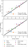 |
Figure 8 Correlation of the results of the rating scale assessment test of the second experiment with the arithmetic average of the sharpness according to Aures (upper figure) and DIN 45692 (lower figure) methods with 95% confidence intervals and Pearson R. Without the monaural signal. |
Even though in the case of the monaural signals the ear channel with the lower sharpness appeared to have only a minor influence on binaural sharpness perception, for nearly all signals it is evident that the maximum value alone – that is, the ear channel with the higher sharpness – can almost never reflect the listening test results. For all signals, this calculation initially predicts an increase in sharpness when the sound source moves from the frontal position towards lateral positions, which was not observed in any of the listening experiments. Therefore, while being able to give an approximate estimate of the sharpness of a signal, a maximum value, as implicitly suggested in the ISO/TS 12913-3 [22], is unsuitable as a representative single-value metric for binaural sharpness, especially regarding different sound source positions. Additionally, the results for the monaural signals suggest that, unlike loudness, sharpness does not exhibit a binaural summation effect, which makes a simple averaging approach more plausible than averaging with a weighting factor based on the assumption of binaural summation as applied by Segura-Garcia et al. [19].
Generally loudness seems to have a particularly strong influence on sharpness in the binaural case, making sharpness calculation and averaging according to the method by Aures a promising approach. While arithmetic averaging as proposed by Klemenz and Fels [18] appears to be suitable, quadratic averaging (RMS) may better reflect the potentially greater contribution of the more dominant channel.
4.3 Method
We relied on self-reported normal hearing when recruiting participants, without conducting formal tests to determine individual hearing levels. Although this may be considered a limitation, all stimuli were presented at sound pressure levels likely well above the hearing threshold. For this case, Kleczkowski et al. [34] did not find a systematic relationship between hearing level and listening test performance. Considering this, as well as the fact that most of the participants were under the age of 35, it is unlikely that non-normal hearing systematically affected the results.
Although paired comparisons are a practical and easily understandable test method for participants, their interpretive power is limited. From paired comparison data, a ratio scale can be obtained by applying the Bradley-Terry-Luce model, which gives them greater interpretative power and enables further analysis [35]. However, this requires strong stochastic transitivity (SST) to hold [29, 30], which was not the case with the data here. In cases of minimal stimulus differences, the forced-choice design, which requires participants to select an option even if no difference is perceived, can lead to arbitrary decisions, reflected in a high number of circular triads and low consistency as observed in the first experiment, thereby making it difficult for SST to hold. Providing a “no difference" option or employing an alternative test design could have yielded more meaningful results. In the rating scale the randomized playback of all signals resulted in a high variance and many participants found the task challenging due to the absence of a reference sound. Despite these limitations, clear effects were observed, unfortunately the reduced number of sound source positions was a drawback. Paired comparison tests proved only partially suitable and adaptive methods may offer more detailed insights on binaural sharpness perception.
Despite the use of non-individualized binaural synthesis in the second experiment, the presence of binaural effects could be demonstrated.
5 Conclusion
The effect of different sound source positions in the horizontal plane on sharpness perception was investigated under two different listening conditions. In an anechoic chamber with stimuli presented via loudspeaker, as well as in a headphone based listening experiment where signals were presented as virtual sound sources. Results were compared to different calculation and averaging approaches for deriving a single value metric for binaural sharpness. The following conclusions can be drawn:
-
In both experiments, sharpness perception decreased with increasing lateral sound incidence angle for broadband signals. This also suggests that sharpness perception can be investigated with non-individual virtual sound sources to reduce the effort for realizing future experiments.
-
In order to compare the overall sharpness of different signals with equal sound incidence angle, conventional single-channel methods (e.g. Aures, DIN 45692) and, for example, the use of the maximum value (channel with the higher sharpness) work well.
-
Even so experiments indicate that the sharpness of the contralateral side has almost no impact on the binaural sharpness percept, considering only the higher channel value cannot adequately represent the perceived sharpness between different sound source positions of one signal. To evaluate different sound source positions of one signal in the horizontal plane in terms of sharpness, arithmetic or quadratic averaging of sharpness calculated according to Aures method seem to be promising approaches that could reflect the experimental results. As loudness seems to have an impact on the binaural sharpness percept, averaging the sharpness of both ear channels calculated after DIN 45692 method, which disregards the influence of loudness on sharpness, did not accurately represent the listening test results.
-
Monaural signals (single ear presentation) appeared to be a special case. Averaging the sharpness values of both channels, gives an incorrect estimate of the perceived sharpness. The findings indicate that unlike loudness, sharpness does not exhibit a binaural summation effect. Future research should investigate this special case further.
Conflicts of interest
The authors declare no conflict of interest.
Data availability statement
Supplementary material such as signals or listening test data are available on request from the author.
References
- D.W. Robinson, L.S. Whittle: The loudness of directional sound fields. Acustica 10 (1960) 74–80. [Google Scholar]
- V.P. Sivonen: Directional loudness and binaural summation for wideband and reverberant sounds. Journal of the Acoustical Society of America 121, 5 (2007) 2852–2861. [CrossRef] [PubMed] [Google Scholar]
- V.P. Sivonen, W. Ellermeier: Directional loudness in an anechoic sound field, head-related transfer functions, and binaural summation. Journal of the Acoustical Society of America 119, 5 (2006) 2965–2980. [CrossRef] [PubMed] [Google Scholar]
- V.P. Sivonen, W. Ellermeier: Binaural loudness for artificial-head measurements in directional sound fields. Journal of the Audio Engineering Society 56, 6 (2008) 452–461. [Google Scholar]
- International Organization for Standardization: ISO 532-2:2017. Acoustics – Methods for calculating loudness. Part 2: Moore-Glasberg method. Standard, 2017. [Google Scholar]
- International Organization for Standardization: ISO 532-3:2023. Acoustics – Methods for calculating loudness. Part 3: Moore-Glasberg-Schlittenlacher method. Standard, 2023. [Google Scholar]
- A. Fiebig, F. Hochbaum, F. Brinkmann: Experimental study on sharpness and roughness sensations with varying source positions in the horizontal plane, in: DAS – DAGA – 51st Annual Meeting on Acoustics, Copenhagen, Denmark, 2025, pp. 1104–1107. [Google Scholar]
- H. Fastl, E. Zwicker: Psychoacoustics: facts and models, 2nd edn, vol. 22. Springer Series in Information Sciences. Springer Nature, Berlin, Heidelberg, 2007. [Google Scholar]
- C. Maschke, A. Jakob: Psychoakustische Messtechnik. In: Möser M, Ed. Messtechnik der Akustik. Springer Berlin Heidelberg, Berlin, Heidelberg, 2009, pp. 599–642. [Google Scholar]
- G.V. Bismarck: Sharpness as an attribute of the timbre of steady sounds. Acustica 30 (1974) 159–172. [Google Scholar]
- W. Aures: Berechnungsverfahren für den Wohlklang beliebiger Schallsignale. Ein Beitrag zur gehörbezogenen Schallanalyse. Dissertation. Technische Universität München, München, 1984. [Google Scholar]
- Deutsches Institut für Normung: DIN 45692:2009-08. Measurement technique for the simulation of the auditory sensation of sharpness. Standard. Beuth Verlag, Berlin, 2009. [Google Scholar]
- A. Fiebig, R. Sottek, V. Tarasova: Wahrnehmung der Schärfe von instationären technischen Schallen. In: Fortschritte der Akustik, DAGA 2008 – Dresden, 2017, pp. 780–783. [Google Scholar]
- W. Ellermeier, J. Hellbrück: Hören – Psychoakustik – Audiologie. In: Weinzierl S, Ed. Handbuch der Audiotechnik. VDI-Buch. Springer, Berlin, Heidelberg, 2008, pp. 41–85. [Google Scholar]
- X.-L. Zhong, F.-C. Zhang, B.-S. Xie: On the spatial symmetry of head-related transfer functions. Applied Acoustics 74, 6 (2013) 856–864. [Google Scholar]
- B. Xie: Head-related transfer function and virtual auditory display, 2nd edn. J. Ross Publishing, Plantation, FL, USA, 2013. [Google Scholar]
- M.H.A. Bunse: Binaurale Rauhigkeit räumlich verteilter Schallquellen. In: Fortschritte der Akustik, DAGA 1993, 1993, pp. 848–852. [Google Scholar]
- M. Klemenz, J. Fels: Zur Berechnung psychoakustischer Grösen mehrerer Schallquellen. In: Fortschritte der Akustik, DAGA 2002 – Bochum, 2002, pp. 502–503. [Google Scholar]
- J. Segura-Garcia, J. Navarro-Ruiz, J. Perez-Solano, J. Montoya-Belmonte, S. Felici-Castell, M. Cobos, A. Torres-Aranda: Spatio-temporal analysis of urban acoustic environments with binaural psychoacoustical considerations for IoT-based applications. Sensors 18, 3 (2018) 690. [Google Scholar]
- B.C.J. Moore, B.R. Glasberg: Modeling binaural loudness. Journal of the Acoustical Society of America 121, 3 (2007) 1604–1612. [Google Scholar]
- International Organization for Standardization: ISO/TS 12913-2:2018. Akustik – Soundscape – Teil 2: Anforderungen an die Datenerhebung und die Dokumentation. Standard, 2018. [Google Scholar]
- International Organization for Standardization: ISO/TS 12913-3:2019. Akustik – Soundscape – Teil 3: Datenanalyse. Standard, 2019. [Google Scholar]
- F. Brinkmann, S. Weinzierl: AKtools – an open software toolbox for signal acquisition, processing, and inspection in acoustics. In: 142nd AES Convention, Berlin, Germany, 2017. [Google Scholar]
- F. Font, G. Roma, X. Serra: Freesound technical demo. In: Proceedings of the 21st ACM international conference on Multimedia, ACM, 2013, pp. 411–412. [Google Scholar]
- A.P. Soares, A.P. Pinheiro, A. Costa, C. Frade, M. Comesaña: Affective auditory stimuli: adaptation of the International Affective Digitized Sounds (IADS-2) for European Portuguese. Behavior Research Methods 45 (2013) 1168–1181. [Google Scholar]
- L. Pires, M. Vieira, H. C. Yehia, T. Brookes, R. Mason: A new set of directional weights for ITUR BS.1770 loudness measurement of multichannel audio. ITU Journal: ICT Discoveries 3, 1 (2020) pp. 101–108. [Google Scholar]
- F. Brinkmann, A. Lindau, S. Weinzierl, S.V.D. Par, M. Müller-Trapet, R. Opdam, M. Vorländer: A high resolution and full-spherical head-related transfer function database for different head-above-torso orientations. Journal of the Audio Engineering Society 65, 10 (2017) 841–848. [CrossRef] [Google Scholar]
- S. Fredelake, I. Holube: Qualitätsbeurteilungen durch Paarvergleich. Zeitschrift für Audiologie 49, 4 (2010) 149–156. [Google Scholar]
- W. Ellermeier, K. Zimmer: Using psychological choice models to investigate overall sound quality. In: First ISCA Workshop on Auditory Quality of Systems, Akademie Mont-Cenis, Germany, 23–25 April 2003, pp. 71–78. [Google Scholar]
- S. Choisel, F. Wickelmaier: Evaluation of multichannel reproduced sound: Scaling auditory attributes underlying listener preference. Journal of the Acoustical Society of America 121, 1 (2007) 388–400. [Google Scholar]
- E. Parizet: Paired comparison listening tests and circular error rates. Acta Acustica United with Acustica 88 (2002), 594–598. [Google Scholar]
- D. Lakens: Calculating and reporting effect sizes to facilitate cumulative science: a practical primer for t-tests and ANOVAs. Frontiers in Psychology 4 (2013) 863. [Google Scholar]
- R. Sottek, J. Becker: Modellierung der psychoakustischen Rauigkeit. In: DAGA 2019 – Rostock, 2019, pp. 832–835. [Google Scholar]
- P. Kleczkowski, M. Pluta, P. Macura, E. Paczkowska: Listeners who have low hearing thresholds do not perform better in difficult listening tasks. In: 132nd AES Convention, Convention Paper 8641, Budapest, Hungary, 2012. [Google Scholar]
- W. Ellermeier, M. Mader, P. Daniel: Scaling the unpleasantness of sounds according to the BTL model: Ratio-scale representation and psychoacoustical analysis. Acta Acustica United with Acustica 90 (2004) 101–107. [Google Scholar]
Cite this article as: Hochbaum F. Hundt T. Fiebig A. Brinkmann F. 2025. Directional sharpness perception under different listening conditions 9, 60. https://doi.org/10.1051/aacus/2025048.
All Tables
Number of remaining participants N and averaged consistency coefficient ζ of the paired comparison tests in the second experiment without participants with a consistency coefficient ζ < 0.6.
Effect sizes (Cohen’s d) for the rating scale results. Bold indicates at least a small effect (|d|≥0.20). Asterisks denote Bonferroni-corrected t-test significance: * p < .05, ** p < .01, *** p < .001.
All Figures
|
Figure 1 Spectrograms (window: Hanning; window length: 1024; window overlap: 50%) of the three signals used in the first experiment (anechoic chamber). |
| In the text | |
|
Figure 2 Full anechoic chamber used for experiment I with the listening position (where the artificial head is mounted) located in the center of the loudspeaker array. |
| In the text | |
|
Figure 3 Spectrograms (window: Hanning; window length: 1024; window overlap: 50%) of the single channel signals (excluding “birds", see Fig. 1) used in the second experiment (audiometry cabin) prior to auralization. |
| In the text | |
|
Figure 4 Audiometry cabin for the execution of experiment II and artificial head measurement system to adjust the playback level. |
| In the text | |
|
Figure 5 Results of the first experiment (anechoic chamber) showing the averaged win rate in the paired comparison tests per signal for the different spatial positions. |
| In the text | |
|
Figure 6 Results of the second experiment (audiometry cabin) showing the averaged win rate in the paired comparison tests for the signals “sharp noise", “birds", and “CB19 sharp noise" for the considered spatial positions (top), the results of sharpness method according to Aures [11] (middle) and the results of sharpness method according to DIN 45692 [12] (bottom). |
| In the text | |
|
Figure 7 Results of the second experiment (audiometry cabin) showing the rating scale assessment results for all signals as mean values with 95% confidence intervals and rating distribution (top), the results of sharpness method according to Aures [11] (middle) and the results of sharpness method according to DIN 45692 [12] (bottom). |
| In the text | |
|
Figure 8 Correlation of the results of the rating scale assessment test of the second experiment with the arithmetic average of the sharpness according to Aures (upper figure) and DIN 45692 (lower figure) methods with 95% confidence intervals and Pearson R. Without the monaural signal. |
| In the text | |
Current usage metrics show cumulative count of Article Views (full-text article views including HTML views, PDF and ePub downloads, according to the available data) and Abstracts Views on Vision4Press platform.
Data correspond to usage on the plateform after 2015. The current usage metrics is available 48-96 hours after online publication and is updated daily on week days.
Initial download of the metrics may take a while.