| Issue |
Acta Acust.
Volume 10, 2026
|
|
|---|---|---|
| Article Number | 4 | |
| Number of page(s) | 6 | |
| Section | Aeroacoustics | |
| DOI | https://doi.org/10.1051/aacus/2025072 | |
| Published online | 06 February 2026 | |
Scientific Article
Aeroacoustic whistling mechanisms in perforated pen caps
Laboratoire d’Acoustique de l’Université du Mans, UMR 6613, CNRS, Le Mans Université, Le Mans, France
* Corresponding author: This email address is being protected from spambots. You need JavaScript enabled to view it.
Received:
22
July
2025
Accepted:
29
December
2025
Abstract
This paper investigates the acoustic behavior of a perforated pen cap, which acts as a compact self-sustained whistling system. Through experimental measurements and numerical simulations, we analyze the aeroacoustic interaction between jet flow dynamics and resonator geometry to identify conditions under which sound generation and amplification occur. The study highlights key aeroacoustic mechanisms and demonstrates pedagogical value, while suggesting practical implications for the design of flow-induced sound devices.
Key words: Whistling / Aeroacoustics / Vortex sound
© The Author(s), Published by EDP Sciences, 2026
 This is an Open Access article distributed under the terms of the Creative Commons Attribution License (https://creativecommons.org/licenses/by/4.0), which permits unrestricted use, distribution, and reproduction in any medium, provided the original work is properly cited.
1 Introduction
The characteristic whistling produced when blowing into a pen cap – such as the BIC® Cristal model – may seem surprising. One might assume that its smooth external form implies a similarly smooth internal geometry. However, blowing through a smooth tube, even conical, does not produce a whistle, unlike corrugated tubes, where this behavior is well documented [1, 2].
Interestingly, previous studies have shown that whistling can also occur in smooth tubes when there is a sudden change in cross-sectional area, such as a sharp expansion [3] or contraction [4] at one end. A detailed examination of the internal geometry of a BIC® Cristal pen cap reveals just such a contraction at its narrower extremity. This abrupt narrowing induces flow separation when air is blown into the cap – an effect that closely resembles the behavior observed in ducts equipped with diaphragms.
Though pen cap acoustics may appear trivial, their origin lies in a crucial safety regulation. Between 1970 and 1984, nine children in the UK fatally choked on pen caps, prompting new standards in 1990. Manufacturers were then required to include air passages to reduce suffocation risk, resulting in the now-familiar perforated caps. The resulting design unintentionally turned pen caps into aeroacoustic resonators.
In this study, we analyze the geometry and acoustic response of a commercial pen cap. Numerical simulations and experimental measurements are used to investigate the physical mechanisms responsible for the observed whistling, with particular attention to flow separation and resonance phenomena to identify the dominant coupling mechanisms.
2 Geometry
In the absence of data on the internal geometry of the pen cap, an internal silicone mould was made and measured. The approximate geometry is given in Figure 1.
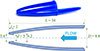 |
Figure 1. Picture and measured internal shape of the of the BIC® Cristal ballpoint pen. |
The important point in Figure 1 is the abrupt reduction in diameter located axially at l = 2 mm from the narrowest outlet. The diameter drops from 4.2 mm to d = 3 mm, then increases slightly towards the outlet, forming a slightly diverging cone. This abrupt change in cross-sectional area induces flow separation when blowing, as is demonstrated numerically in the following section.
3 Numerical simulations and vortex sound
Numerical simulations of the steady flow field inside the pen cap were performed using COMSOL® Multiphysics, employing a Reynolds-Averaged Navier–Stokes (RANS) model for a mean velocity U 0 = 20 m s−1. The resulting velocity field is presented in Figure 2a. This computation was performed for various mean flow velocities ranging from 10 to 50 m s−1. The overall flow pattern was found to be nearly independent of the flow velocity.
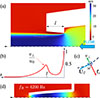 |
Figure 2. (a) Numerical simulation of the axial mean velocity field within the pen cap contraction for a mean velocity U 0 = 20 m s−1. The black dashed line indicates the position of the shear layer. (b) Amplitude of the acoustic velocity component v ⊥, perpendicular to the shear layer, normalized by the mean acoustic velocity in the contraction u 0. (c) Schematic representation of the vorticity ω, the mean tangential velocity U Γ, and the normal acoustic velocity v ⊥. (d) Acoustic pressure field at the first resonance. |
The simulation clearly reveals a flow separation occurring at the entrance of the geometric contraction, leading to the formation of a jet. A well-defined shear layer develops at the interface between the jet and the surrounding fluid where vorticity is strongly concentrated. Figure 2a highlights this region with a dashed line.
To model the coupling between acoustics and the flow field, as the Mach numbers are low, the Powell–Howe analogy is employed [5, 6]. The time-averaged acoustic power generated by the flow within a volume V is given by:
 (1)
(1)
where ⟨·⟩ denotes time averaging, va is the acoustic velocity (i.e., the potential part of the fluctuating velocity), and fc is the Coriolis-like force acting on a fluid particle due to flow rotation, expressed as
 (2)
(2)
with ρ0 the ambient density, ω the vorticity of a fluid particle and UΓ the total velocity of this fluid particle.
When an acoustic field is superimposed on the mean flow, the vorticity shed from the separation point (i.e., the upstream edge of the contraction) becomes modulated by the acoustic oscillations. This perturbation adds to the mean vorticity and is primarily convected along the shear layer, where it is amplified by a Kelvin–Helmholtz instability [7, 8].
As a result, each fluid particle within the shear layer is subjected to a Coriolis-like force that acts perpendicular to the shear layer. The direction of this force is determined by the sign of the mean acoustic velocity u 0 at the entrance of the contraction at the moment the vorticity is shed, since the sign of the particle’s vorticity remains unchanged as it is convected along the shear layer.
For instance, when the acoustic velocity is directed outward from the cap, a fluid particle leaving the upstream edge acquires a positive vorticity, and the resulting Coriolis force is oriented toward the jet (see Fig. 2c).
In equation (1), both the Coriolis force and the acoustic velocity va must be determined. At low Mach numbers, the influence of the mean flow on the acoustic field can be neglected. Therefore, the acoustic velocity can be obtained from a numerical simulation performed without mean flow. Using the Acoustics Module in COMSOL®, the acoustic pressure and velocity fields v a were computed under the assumptions of no mean flow and negligible visco-thermal losses. The first resonance frequency f R was found to be 4200 Hz, which is close to that of an ideal open-open tube, for which λ/2 = c 0/(2f R )=L, where c 0 is the speed of sound and L the length of the cap. The corresponding pressure field at resonance is shown in Figure 2d.
Figure 2b displays the component of the acoustic velocity normal to the shear layer, v⊥, plotted as a function of the curvilinear coordinate s (which closely approximates the axial coordinate x) at the pen cap’s resonance frequency. Since the size of the region of interest (of the order of l) is small compared to the acoustic wavelength, compressibility effects are weak, and an incompressible calculation would have yielded a very similar result for v ⊥. The simulation also reveals the presence of two distinct regions where the normal acoustic velocity is significantly large: one near the upstream edge of the contraction, and another near the outlet of the cap, the latter being due to the radial acoustic velocity associated to the acoustic radiation at the cap exit.
In the first region, located near the upstream edge of the contraction, the acoustic power generation is negative, indicating that sound is absorbed by the flow. This occurs because, during the half-cycle when the acoustic velocity is directed outward from the cap, the Coriolis force f c is directed toward the jet, while the normal acoustic velocity v ⊥ points outward – yielding a negative contribution to the acoustic power f c ⋅ v a . During the opposite half-cycle, both vectors reverse direction, but their scalar product remains negative. Thus, this region consistently acts as an acoustic energy sink.
To produce a sustained whistling sound, the flow must not only generate more acoustic energy than is absorbed in the upstream dissipation region, but also compensate for the acoustic losses at the resonance of the cap, which behaves as an open–open duct. At the resonance frequency, these losses are mainly due to acoustic radiation at the duct openings and to visco-thermal dissipation within the cap. Such a net positive acoustic power balance is only possible in regions where the amplitude of the normal acoustic velocity v⊥ is significant – namely, near the outlet of the cap. The location of the acoustic production region is outlined by an orange dashed oval in Figure 2a.
In order for acoustic energy to be generated in this region, a fluid particle that initially acquired a positive vorticity due to a positive mean acoustic velocity u 0 must arrive near the cap outlet at a time when the acoustic velocity has reversed direction. In that case, the Coriolis force and v⊥ have the same direction, and their scalar product becomes positive, resulting in local acoustic power generation.
Moreover, the spatial and temporal integral of this power density over both the source and sink regions must be positive and sufficiently large to overcome the intrinsic acoustic losses of the resonator.
Then, the key parameter governing the potential for whistling is the ratio between the time tΓ required for a vorticity perturbation to travel from the upstream edge of the contraction to the outlet of the cap, and the acoustic period T = 1/fR. The time tΓ is proportional to the length l of the contraction and inversely proportional to the velocity of the vorticity perturbations, which scales with the mean flow velocity U0. Therefore, the relevant dimensionless number in this context is the Strouhal number:
 (3)
(3)
It has been shown that, for a diaphragm in a duct [9], there exists a range of potential whistling frequencies, defined as those associated with a production of acoustic energy. This whistling potential typically occurs around a Strouhal number in the range of 0.2–0.35. A second region of potential whistling exists around St = 0.75, corresponding to the second hydrodynamic mode, which arises when a vorticity perturbation takes two acoustic periods to travel across the diaphragm. Experiments in a resonant environment have demonstrated that whistling is triggered when one of the duct’s resonance frequencies lies within the range of potential whistling frequencies [10].
4 Experimental results for sound production
A cap from a BIC® Cristal pen was mounted at the downstream end of a straight cylindrical tube with an inner diameter of 30 mm, see Figure 3a. No active excitation was applied, and the tube terminated upstream with an anechoic end condition to minimize acoustic reflections. The sound generated by the cap was recorded externally using a B&K 4136 microphone coupled with a Nexus 2690 amplifier. The microphone was positioned 1 cm downstream (axially) and 6 cm away (radially) from the end of the cap, perpendicular to the axis of the tube. The mean flow is provided by a centrifugal pump and its velocity U0 in the contraction was estimated by measuring the mass flow rate through the tube and dividing it by the cross-sectional area of the narrowest part of the contraction (diameter d = 3 mm). Note that the maximum airflow rate in this measurement is approximately 0.3 liters per second, which corresponds to a flow rate that can easily be achieved by blowing with the mouth.
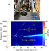 |
Figure 3. (a) Photograph of the experimental setup. (b) Spectrogram of the emitted sound as a function of the mean flow velocity U0. The dotted line corresponds to first resonance frequency fR = 4200 Hz. The dashed line corresponds to a constant Strouhal number St = 0.74. |
The microphone measurements are presented as a spectrogram in Figure 3b, as a function of the mean flow velocity U0, which was gradually increased during the experiment. A measurement was also performed while decreasing the velocity, but the results did not differ significantly from those shown. It can be noted that slight geometrical differences between the caps may influence the ease of excitation and the occurrence of the second resonance.
A first low-amplitude whistling appears for U 0 between 10 and 14 m s−1. The frequency of this tone is close to the resonance frequency f R of the cap but varies linearly with the flow velocity. As shown in Figure 3b, it remains very close to the line corresponding to St = 0.74. The value of the Strouhal number suggests that this corresponds to the second hydrodynamic mode [9].
This first whistling thus behaves like an edge tone that is only weakly coupled to the acoustic resonance. The feedback mechanism is essentially hydrodynamic: when vorticity perturbations, amplified within the shear layer, reach the vicinity of the cap outlet, they induce pressure fluctuations that act quasi-instantaneously on the separation point through an incompressible feedback process. The acoustic field has very little effect on the generation of these vorticity perturbations. It primarily serves to amplify the hydrodynamic sound production when the frequency approaches resonance conditions. This type of behavior has already been observed in organ pipes, where, at low flow velocities, the oscillation frequency initially increases proportionally with the velocity before locking onto the pipe’s acoustic resonance frequency [11, 12].
A second weak whistling is observed for U 0 between 20 and 25 m s−1. Its frequency is close to 2f R and also varies with the flow velocity in such a way that the Strouhal number remains nearly constant at St = 0.74. This tone is thus likely associated with the second hydrodynamic mode, this time weakly coupled to the second acoustic resonance of the cap.
For flow velocities above 25 m s−1, a third and much stronger whistling emerges. Its frequency abruptly shifts to the fundamental acoustic resonance of the cap, f R , corresponding initially to St = 0.34. As the velocity increases further, the amplitude of this whistling grows significantly, reaching a maximum near U 0 = 35 m s−1 (St = 0.21), before gradually decreasing and eventually vanishing. This dominant whistling is the most intense of the three and is typically the one heard when no particular care is taken to control the airflow – making it the most easily perceived in casual use.
5 Discussion and conclusion
The BIC pen cap provides a simple yet effective example of an aeroacoustic system in which geometry, flow, and acoustic resonance interact to produce audible tones. Due to its widespread use and low cost, it can serve as an accessible educational tool to illustrate the phenomenon of flow-induced whistling in ducts.
This study highlights that flow-induced whistling can occur even in the absence of vortex impingement on a sharp edge. A key point is the importance of flow separation and the presence of a significant normal acoustic velocity component, v ⊥, in the shear layer downstream of the separation point. This is illustrated in Figure 4.
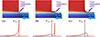 |
Figure 4. In the top row of figures, the background color represents the mean axial velocity, computed using RANS simulations, while the streamlines correspond to the acoustic velocity field calculated assuming an inviscid fluid. The bottom row shows the component of the acoustic velocity normal to the jet (i.e., radial velocity). These plots are presented for three geometries: (a) a straight pipe, (b) a pipe with an expansion, and (c) a pipe with a rounded outlet. |
In the case of a straight pipe (Fig. 4a), |v⊥| decreases monotonically downstream, and no whistling occurs – on the contrary, some acoustic energy is absorbed by the flow. In contrast, for a pipe with an expanded outlet (Fig. 4b), a maximum of |v⊥| appears downstream of the separation point, allowing whistling to develop. The same applies to the rounded outlet configuration (Fig. 4c), where |v⊥| also peaks beyond the separation point. Interestingly, this configuration closely resembles human whistling, where flow separation occurs over the rounded geometry of the lips [13]. The analogy highlights the generality of the mechanisms described. These are also examples where whistling occurs without any direct vortex-edge interaction.
The study also reveals that the whistling phenomenon is highly sensitive to small geometric details, such as the small internal protrusion inside the pen cap. This strong sensitivity suggests potential design strategies for suppressing unwanted flow-induced tones: even slight geometric modifications may be sufficient to disrupt the coupling mechanism and render the system quieter.
Overall, this study demonstrates how even common objects like pen caps can serve as effective models for exploring complex aeroacoustic phenomena – with implications for both pedagogy and noise control design.
Cite this article as: Aurégan Y. 2026. Aeroacoustic whistling mechanisms in perforated pen caps. Acta Acustica, 10, 4. https://doi.org/10.1051/aacus/2025072.
Acknowledgments
The author warmly thanks Patrick BLANC from TechnicAtome for asking a deceptively simple question: “By the way, why do pen caps whistle?” A question that ultimately sparked this study.
Funding
The author received no funding to complete this research.
Conflicts of interest
The author declares no conflicts of interest.
Data availability statement
The data are available upon request from the author.
References
- G. Nakiboğlu, S. Belfroid, J. Golliard, A. Hirschberg: On the whistling of corrugated pipes: effect of pipe length and flow profile. Journal of Fluid Mechanics 672 (2011) 78–108. [Google Scholar]
- M.E. D’Elia, T. Humbert, Y. Aurégan: Linear investigation of sound-flow interaction along a corrugated plate. Journal of Sound and Vibration 534 (2022) 117048. [CrossRef] [Google Scholar]
- A. Hirschberg, J. Bruggeman, A. Wijnands, N. Smits: The “whistler nozzle” and horn as aero-acoustic sound sources in pipe systems. Acta Acustica united with Acustica 68 (1989) 157. [Google Scholar]
- A. Anderson: Dependence of pfeifenton (pipe tone) frequency on pipe length, orifice diameter, and gas discharge pressure. Journal of the Acoustical Society of America 24 (1952) 675. [Google Scholar]
- A. Powell: Theory of vortex sound. Journal of the Acoustical Society of America 36 (1964) 177. [Google Scholar]
- M. Howe: Contributions to the theory of aerodynamic sound, with application to excess jet noise and the theory of the flute. Journal of Fluid Mechanics 71 (1975) 625. [Google Scholar]
- S. Dequand, S. Hulshoff, A. Hirschberg: Self-sustained oscillations in a closed side branch system. Journal of Sound and Vibration 265 (2003) 359. [Google Scholar]
- S.W. Rienstra, A. Hirschberg: An Introduction to Acoustics. Technische Universiteit Eindhoven, 2004. [Google Scholar]
- P. Testud, Y. Aurégan, P. Moussou, A. Hirschberg: The whistling potentiality of an orifice in a confined flow using an energetic criterion. Journal of Sound and Vibration 325 (2009) 769. [CrossRef] [Google Scholar]
- R. Lacombe, P. Moussou, Y. Aurégan: Whistling of an orifice in a reverberating duct at low mach number. Journal of the Acoustical Society of America 130 (2011) 2662. [CrossRef] [PubMed] [Google Scholar]
- J.W. Coltman: Jet drive mechanisms in edge tones and organ pipes. Journal of the Acoustical Society of America 60 (1976) 725. [CrossRef] [Google Scholar]
- M.-P. Verge, B. Fabre, A. Hirschberg, A. Wijnands: Sound production in recorderlike instruments. I. Dimensionless amplitude of the internal acoustic field. The Journal of the Acoustical Society of America 101 (1997) 2914. [Google Scholar]
- T.A. Wilson, G.S. Beavers, M.A. DeCoster, D.K. Holger, M.D. Regenfuss: Experiments on the fluid mechanics of whistling. The Journal of the Acoustical Society of America 50 (1971) 366. [Google Scholar]
Cite this article as: Aurégan Y. 2026. Aeroacoustic whistling mechanisms in perforated pen caps. Acta Acustica, 10, 4. https://doi.org/10.1051/aacus/2025072.
All Figures
|
Figure 1. Picture and measured internal shape of the of the BIC® Cristal ballpoint pen. |
| In the text | |
|
Figure 2. (a) Numerical simulation of the axial mean velocity field within the pen cap contraction for a mean velocity U 0 = 20 m s−1. The black dashed line indicates the position of the shear layer. (b) Amplitude of the acoustic velocity component v ⊥, perpendicular to the shear layer, normalized by the mean acoustic velocity in the contraction u 0. (c) Schematic representation of the vorticity ω, the mean tangential velocity U Γ, and the normal acoustic velocity v ⊥. (d) Acoustic pressure field at the first resonance. |
| In the text | |
|
Figure 3. (a) Photograph of the experimental setup. (b) Spectrogram of the emitted sound as a function of the mean flow velocity U0. The dotted line corresponds to first resonance frequency fR = 4200 Hz. The dashed line corresponds to a constant Strouhal number St = 0.74. |
| In the text | |
|
Figure 4. In the top row of figures, the background color represents the mean axial velocity, computed using RANS simulations, while the streamlines correspond to the acoustic velocity field calculated assuming an inviscid fluid. The bottom row shows the component of the acoustic velocity normal to the jet (i.e., radial velocity). These plots are presented for three geometries: (a) a straight pipe, (b) a pipe with an expansion, and (c) a pipe with a rounded outlet. |
| In the text | |
Current usage metrics show cumulative count of Article Views (full-text article views including HTML views, PDF and ePub downloads, according to the available data) and Abstracts Views on Vision4Press platform.
Data correspond to usage on the plateform after 2015. The current usage metrics is available 48-96 hours after online publication and is updated daily on week days.
Initial download of the metrics may take a while.