© The Author(s), Published by EDP Sciences, 2026

1. Introduction

Bowed-string instruments have evolved over centuries, culminating in the various designs of today’s musical scenes and practices. Their sound originates from the frictional interaction between the bow hairs and the string, inducing string oscillations that are transferred to and emitted by the instrument body. The understanding of the associated stick-slip behaviour was pioneered by Helmholtz [1] and Raman [2], and has steadily advanced since.

A critical part of any bowed-string model is how the friction force is defined. The earliest computer simulation efforts assumed that the string switches between two distinct states, slipping and sticking, with the coefficient of friction decreasing with sliding speed [3–5], which in other contexts is often referred to as the “Stribeck effect” [6]. In a push to improve the predictive capability of such “friction curve models”, studies were undertaken to determine a suitable mathematical expression for this dependency, either by curve fitting to steady-sliding measurement data such as presented in [7, 8] or using theory to derive a friction curve from measured bridge force transients [9]. Concurrently, experimental evidence pointed to hysteresis occuring during stick-slip cycles, prompting a radically different approach in which the coefficient of friction depends on the contact temperature of the interfacial layer of rosin¹ instead of the sliding speed [8]. The additional ingredient required is a heat-balance equation that models the evolution of the contact temperature. The “thermal model” proposed along this principle shows an improved match with measurement compared to friction curve models, in both the Schelleng plane and the Guettler plane [10–12].

The state of the art is to define the coefficient of friction as a function of both sliding speed and contact temperature [13, 14], thus featuring two state variables and in that sense resembling so-called “rate-and-state models” [15]. In addition, this recently developed “enhanced thermal model” makes use of measured bridge force signals to calibrate the size of the drop in relative velocity during the first slip. The main advantage over the original thermal model is that it is far better at reproducing the rapid change of rate typically observed at the onset of the first slip in bridge force signals when a relatively large bowing force is applied. To illustrate the fast change of rate, three example measured bridge force waveforms are shown in Figure 1a. Doing a better job in getting the first slip right was shown to result in improved simulation of transients [13].

Figure 1. (a) Example initial transients of a bridge force signal measured with a cello G string and a bow acceleration of 0.1 m/s2. The values of the bowing force and relative bow-bridge distance are f b = 4.1 N, x b/L = 0.0456 (blue line); f b = 5.2 N, x b/L = 0.0320 (green line); f b = 6.7 N, x b/L = 0.0284 (red line). The grey-shaded region highlights the first slip. (b) Zoom-in at the time of the first slip. The black circles indicate the sampled-data points, which are spaced at 20 μs intervals. (c) Waveform of the steady-state regime, during which the bow velocity was held constant at v b = 0.1 m/s. (d) Zoom-in of the slipping phase.

The mechanism by which the enhanced thermal model is able to reproduce a fast change of rate in the bridge waveform is related to how indeterminacy can arise in modelling dry friction between rigid bodies [16, 17]. In bowed-string dynamics this phenomenon can be explained via graphical construction [18]. As a consequence, the distinction between slipping and sticking has to be explicitly managed. In contrast, with the original thermal model stick-slip behaviour naturally arises from the model equations, but reportedly the absence of a Stribeck characteristic precludes accurate modelling of the initial slip. Both the friction curve model and the enhanced thermal model apply the hysteresis rule proposed in [4] to resolve the indeterminacy. This is manifested as an abrupt jump in the string velocity and as an instantaneous change of rate in the bridge force signal. Such a non-smooth systems approach can be argued to be both reasonable and practical on the grounds that the time scale of the velocity jump is small compared to the shortest relevant period of oscillation. However, bridge force signals sampled at a rate just sufficient to cover the audio bandwidth typically feature a slightly rounded corner at the start of the first slip, as clearly visible in the zoom-in seen in Figure 1b. This raises the question whether some of the transient detail (e.g. the timing of the first slip) is affected by enforcing artifically steep velocity jumps. Given that similarly rapid velocity jumps occur during steady-state oscillation (e.g. Helmholtz motion as shown in Fig. 1c), implementing velocity abruptness may potentially also influence what kind of oscillation regime is sustained for a specific set of bowing parameters. It is therefore of interest to note that evidence presented in [19] reporting on experiments involving bowing a string with a rosin-coated glass rod also points to the transition from sticking to sliding taking place over a short but observable length of time. The explanation offered in [19] is that shear deformation must be taking place in the rosin layer. The significance of enforcing abrupt velocity changes is difficult to assess a priori because a bowed string is a highly nonlinear system displaying a level of sensitive dependency that suggests it operates at the edge of chaos [13, 20]. The implication is that there may be merit in pursuing a complementary modelling strategy that retains the dependence on sliding velocity but resolves fast string velocity transitions in finite time.

Indeed one branch of bowed-string modelling has followed such an approach [21–23], using the “elasto-plastic friction model” proposed in [24, 25] that defines the friction force on basis of a bristle analogy, and inherently incoporates pre-sliding and hysteresis. The distinction between slipping and sticking is made more fuzzy by explicitly incorporating partial slipping. This friction model and its better known forerunner, the “LuGre model” [6, 26], have been developed in a control systems context and are strongly phenomenological in the sense that the model parameters are typically inferred from oscillatory experiments rather than calculated from directly available or measureable material and geometrical constants. In application to stringed instruments, close matches with measured bridge force transients were achieved in [27] by separately optimising the friction parameters for each set of bowing parameters; a reasonably good Guettler diagram match obtained with a single set of friction parameters showed further promise. More recently, guaranteed passivity was shown to be possible via a small and practical model refinement, and solution uniquenes (i.e. determinacy) was formally proven for a simplified case study, the bow-mass model [28]. However the role of the contact temperature cannot be explained with the elasto-plastic model, because the state (the bristle displacement) decreases with the rate (the sliding speed), so the same goes for potential energy stored in the bristles. This implies that the bristle displacement cannot be interpreted as modelling the thermal energy in the contact layer, given that this must increase with sliding speed.

The current article sets out to bridge the gap between elasto-plastic and thermal models. A first step in this direction was made in [29], by adapting the steady-state friction curve acccording to how the viscosity of rosin decresases with temperature. Simulations showed improved behaviour compared to the original elasto-plastic model, in particular displaying more realistic hysteresis behaviour. What is still lacking is a physical explanation of how the elasto-plastic formulation applies to bow-string interaction, as well as a formal proof of solution uniquenesss for the distributed case involving a string rather than a mass. In addition, the heat-balance equation proposed in [29] is heavily simplified, and needs a revision that takes into account its relationship to the model’s steady-sliding behaviour before rigorous validation via comparison with measurement can be undertaken.

The contribution of the present study consists of precisely these steps. In Section 2 a revised thermal elasto-plastic friction formulation is detailed within the larger setting of a bowed-string model featuring torsional string motion, bow-hair compliance, and a finite-width bow. To more easily incorporate accurate frequency-dependent damping, the string equations are cast in modal form, as previously opted for in [30, 31]. The Picard-Lindelöf theorem is applied to prove that the set of ordinary differential equations with which the system can be described has a unique solution. In Section 3 bridge force signals obtained with simulations are analysed alongside measured signals across a grid of bowing positions and bowing forces. Classification on a steady-state part of these signals is carried out to facilitate validation via comparison of the corresponding Schelleng diagrams.

2. Bowed-string model

The sound of bowed-string instruments is articulated by the musician through several left-hand and right-hand manipulations. The frictional contact between the bow and the string is shaped mainly via four variables, namely the bow velocity (the velocity of the bow stick v _b in m/s), the bowing force (the normal force applied to the bow f _b >  0 in N), the bowing position (the position x _b of the bow hair along the string axis, in meters, with the bridge positioned at x = 0), and the bow tilt (the angle between the bow-hair surface and the string axis). During performance, all four of these are time-varying quantities. For the purposes of investigating bow-string friction it is useful to consider a simplified scenario with zero tilting angle and a time-invariant bowing force and bowing position. In other words, the only articulation parameter that remains time-varying is the bow velocity. The proposed model equations are set out accordingly below, where ∂ _x y and d _x y denote the partial and total derivatives of y with respect to x, respectively.

2.1. Equations of motion

Consider a string of length L, radius r, mass density ρ, bending stiffness B, and tension T in contact with a bow of bow-hair width W _b. Hence contact exists across a finite-width region ℬ = [x _b − W _b/2, x _b + W _b/2]. Because with no bow tilt the normal force per unit length F _b = F _b(t) can be assumed to be evenly distributed over the bow hair width, it follows that F _b(t)=f _b(t)/W _b. The string is assumed to be pulled by the bow hairs both transversally and torsionally, and the bow hairs are considered axially compliant. Including stiffness and damping terms, the equations of motion for this system can be stated as [27, 32]:

$$\begin{array}{cc}\hfill \rho A{\partial }_t^{2}u& =T{\partial }_x^{2}u-B{\partial }_x^{4}u-2\rho A\zeta {\partial }_{t}u+\mathcal{F},\hfill \end{array}$$(1)

$$\begin{array}{cc}\hfill P_{\mathsf{T}}{\partial }_t^2\theta & =K_{\mathsf{T}}{\partial }_x^2\theta -2P_{\mathsf{T}}{\zeta }_T{\partial }_t\theta +r\mathcal{F},\hfill \end{array}$$(2)

$$\begin{array}{cc}\hfill D_{\mathrm{h}}{\partial }_t^{2}q& =-K_{\mathrm{h}}q-{\zeta }_{\mathrm{h}}{\partial }_{t}q-F,\hfill \end{array}$$(3)

where u = u(x, t) denotes the transversal string displacement (in m), θ = θ(x, t) is the distributed angular displacement (in radians), and q = q(x, t) is the distributed bow hair displacement relative to the bow stick (in m). The torsional displacement (in m) of a point on the string surface is w(x, t)=r θ(x, t). Simply supported boundary conditions are assumed:

$$\begin{array}{cccccc}\hfill u(0,t)& =0,\hfill & \hfill {\partial }_x^{2}u(0,t)& =0,\hfill & \theta (0,t)& =0,\end{array}$$(4)

$$\begin{array}{cccccc}\hfill u(L,t)& =0,\hfill & \hfill {\partial }_x^{2}u(L,t)& =0,\hfill & \theta (L,t)& =0.\end{array}$$(5)

The bow hair displacement q and the friction force per unit length F (in N/m) are defined only over ℬ, while both u and θ are defined over the domain 𝒮 = [0, L]. Hence over ℬ, ℱ = ℱ(x, t) equals the friction force per unit length F(x, t), while being zero outside this region.

The bow stick is modelled as a rigid object and assumed to move with velocity v _b = v _b(t) along the same axis as the bow hairs. When positive-valued, the friction forces locally pull and rotate the string in positive u and θ direction, respectively, while acting upon the bow hairs in the opposite direction. Hence for x ∈ ℬ, the bow hair velocity is v _b + ∂ _t q, and the (distributed) relative velocity v = v(x, t) between the bow hair and the string is

$$\begin{array}{c}\hfill v=[v_{\mathrm{b}}+{\partial }_{t}q]-[{\partial }_{t}u+r{\partial }_t\theta ].\end{array}$$(6)

The parameter A = π r ² denotes the string’s cross-sectional area, while P _T is the polar moment of inertia, and K _T the torsional stiffness. The bow hairs are characterised by the linear density D _h and the distributed stiffness K _h, while ζ _h is a damping constant. The terms ζ and ζ _T also denote damping, for the transversal and torsional string polarisations, respectively, but – for the purposes of modelling frequency-dependent damping – are not considered as constants; it is in principle possible to use spatial operators for this purpose (see, e.g. [33]), but this is omitted here as accurate frequency-dependence is more conveniently defined directly in the modal domain (see Sect. 2.3).

2.2. Dynamic friction force

A dynamical formulation of a distributed friction force based on the bristle analogy can be stated as follows:

$$\begin{array}{c}\hfill F=\mathrm{\Phi }[{\sigma }_{0}z+{\sigma }_1{\partial }_{t}z+{\sigma }_{2}v],\end{array}$$(7)

where z = z(x, t) denotes the bristle displacement defined over x ∈ ℬ, σ ₀ is the bristle stiffness, σ ₁ is a bristle damping constant, and σ ₂ is a viscous damping constant. Equation (7) incorporates several dynamic friction models appearing in the literature, including the LuGre model [26, 34], the elasto-plastic model [24, 25], and a specific form of the Dahl model [6, 35]. A key distinction across these three models is captured in (7) with the term Φ. That is, for Φ = 1 equation (7) is equivalent to that used in the models used in earlier studies [21, 22, 27], with the coefficient σ ₀ given in N m⁻². The amended form proposed in [36], which in the friction literature is known to be more suited to non-constant normal forces [37], is recovered by choosing Φ = F _b in which case the coefficients become force-per-unit-length-normalised. Given that for bowed strings, friction occurs across a range of normal load values, the amended model is employed here.

Authors focusing on other applications (e.g. [38]) have questioned the need for introducing the bristle damping term in (7). From extensive testing using the bow-string simulation algorithms developed in previous studies [28, 29], it was found that for realistic model parameters both the bristle damping and viscous damping have only a marginal influence on the model’s behaviour, and as such are expected to be negligible in comparison to temperature effects incorporated in the current study. Hence in the remainder of this document both terms will be omitted, writing the friction force per unit length as

$$\begin{array}{c}\hfill F=F_{\mathrm{b}}{\sigma }_{0}z.\end{array}$$(8)

The equation that relates the bristle displacement to the other state variables, which in the friction literature normally only comprises the relative velocity but here also includes the contact temperature, is²

$$\begin{array}{c}\hfill {\partial }_{t}z=v[1-\alpha (z,v,\tau )\frac{z}{z_{\mathsf{ss}}(v,\tau )}]·\end{array}$$(9)

As shown in Appendix C, this equation can be understood as formulating a hysteretic relationship between stress and strain in the rosin layer. The term α(z, v, τ) is sometimes referred to as the “adhesion map” [21, 22], and will be explained shortly. The frictional characteristics are largely embedded within the term z _ss(v, τ), which for v ≠ 0 takes the form

$$\begin{array}{c}\hfill z_{\mathsf{ss}}(v,\tau )=\frac{y(\tau ){\mu }_{\mathsf{str}}(v)}{{\sigma }_0},\end{array}$$(10)

and equals the bristle displacement when z is time-invariant. The function μ _str(v) in equation (10) is a friction curve that imparts a Stribeck effect, while the “temperature factor” y(τ) models how the coefficient of friction depends on the contact temperature above ambient τ (i.e. the temperature in degrees Celsius is τ + 20, assuming the ambient temperature is around twenty degrees). Such a thermal effect can be theorised to arise due to changing material properties in a thin contact layer of the rosin as it undergoes melt lubrication during sliding, i.e. transitions from solid to fluid behaviour [8]. Even though a rigorous explanation of the relevant physical mechanisms has remained somewhat elusive and may require micro-scale analysis, on a macroscopic level one can nonetheless expect y(τ) to range between unity, that holds at ambient temperature, and some positive value y _a <  1 that is taken on at temperatures just beyond the highest observed in bowing cycles.

Qualitatively, μ _str(v) can be expected to have the same antisymmetric characteristics as standard curves employed in friction problems (see Fig. 2 for an example shape). More specifically, it must hold for passivity reasons that v ⋅ μ_str(v)≥0. Further, given that viscous effects are usually considered small in the context of bow-string friction, it is expected that |μ_str| decreases monotonically and quasi-exponentially with |v|, has a maximum μ_s for |v|→0, and reaches μ_d ≤ μ_s in the limit of |v|→∞. For v = 0, which includes the possibility of stiction, the right-hand side of equation (9) vanishes, so both the term z_ss(v, τ) and the friction curve μ_str(v) then become irrelevant, although for non-zero bowing forces the effective friction coefficient can still be calculated as F/F_b = σ₀z.

Figure 2. Expected shape of the friction curve μ str(v).

Unfortunately, the curve μ _str(v) is not directly measurable, because in any experiment with periods of non-zero sliding velocity, the temperature would temporarily rise above ambient temperature, which would modify the observed coefficient of friction. It can however be argued that μ _s should equal the maximum friction coefficient observed in experiments with a constant normal force in which the friction force is gradually increased by moving the bow, which – with knowledge of the bowing position – can be deduced from a measured bridge force signal [9]. In that case, the contact temperature has barely risen above ambient temperature before the first slip, and the value of the friction force reaches f _b μ _s just before slipping. The data gathered from the experiments with a rosin-coated rod reported in [8] pointed to μ _s being fixed at around 1.2. The results reported in [12] and [39] both indicate a significant dependence on bow acceleration in certain regions of the Guettler plane, but with strongly differing average values of the limiting coefficient of friction. A parameterised form of μ _str(v) will be defined in Section 2.2.6 together with (and in relation to) the temperature factor function y(τ) and a measureable steady-state friction curve.

2.2.1. Elasto-plastic friction

What distinguishes the elasto-plastic model from the LuGre model is the inclusion of an adhesion map in (9), which in a thermal friction model takes the form [29]

$$\begin{array}{c}\hfill \alpha (z,v,\tau )=\{\begin{array}{cc}0,\hfill & vz\le 0\hfill \\ {\alpha }_{\mathrm{m}}(z,v,\tau ),\hfill & vz>0\hfill \end{array},\end{array}$$(11)

with

$$\begin{array}{c}\hfill {\alpha }_{\mathrm{m}}(z,v,\tau )=\{\begin{array}{cc}0,\hfill & |z|\le z_{\mathrm{b}\mathrm{a}}\hfill \\ {\overline{\alpha }}_{\mathrm{m}}(z,v,\tau )\hfill & z_{\mathrm{b}\mathrm{a}}<|z|<|z_{\mathsf{ss}}(v,\tau )|\hfill \\ 1\hfill & |z|\ge |z_{\mathsf{ss}}(v,\tau )|\hfill \end{array},\end{array}$$(12)

and

$$\begin{array}{cc}\hfill {\overline{\alpha }}_{\mathrm{m}}(z,v,\tau )& {\displaystyle =\frac{1}{2}[sin(\pi {\theta }_{\mathrm{m}})+1],}\hfill \end{array}$$(13)

$$\begin{array}{cc}\hfill {\theta }_{\mathrm{m}}& =\frac{{\displaystyle |z|-\frac{1}{2}\left(|z_{\mathsf{ss}}(v,\tau )|+z_{\mathrm{b}\mathrm{a}}\right)}}{|z_{\mathsf{ss}}(v,\tau )|-z_{\mathrm{b}\mathrm{a}}}·\hfill \end{array}$$(14)

The value of the so-called break-away value z _ba must be chosen such that it is always smaller than |z _ss(v, τ)|, which is a time-varying quantity. Therefore a logical choice is z _ba = χ z _d(τ), where 0 ≤ χ ≤ 1 and z _d(τ)=y(τ)μ _d/σ ₀ <  |z _ss(v, τ)| for all v. A LuGre friction model is obtained by setting α(z, v, τ)=1. The main significance of the adhesion map is that its inclusion ensures that spurious drift observed with the LuGre model is avoided [24, 25].

2.2.2. Contact area

Figure 3 provides a cross-sectional view of how the bow hairs wrap around the string. Rather than modelling individual bow hairs, following [27, 32] we treat the hairs as forming a ribbon surface that makes contact with the string surface across the bow-hair domain (x ∈ ℬ). With vertical string motion omitted from the model we assume that the string remains straight in that polarisation, and the contact area is then rectangular and increasing with bowing force. For simplicity, it is assumed that the bow-hair tension does not increase when pressure is applied to the bow, and as mentioned before the bow stick is considered as rigid. The bowing force per unit length then divides as [1 − ν]F_b at the tip and νF_b at the frog, where ν is the relative position along the bow axis taking ν = 0 as the tip. At either end of the contact arc, the bow-hair slope must equal the slope of the circular string curvature:

Figure 3. Contact region between the rosin-coated bow hairs and the string. The red part of the line indicates the arc length of contact l c.

$$\begin{array}{cccc}\hfill tan({\varphi }_1)& =\frac{[1-\nu ]F_{\mathrm{b}}}{{\mathcal{T}}_{\mathrm{b}}},\hfill & \hfill tan({\varphi }_2)& =\frac{\nu F_{\mathrm{b}}}{{\mathcal{T}}_{\mathrm{b}}},\hfill \end{array}$$(15)

where 𝒯_b is the tension per unit length (N m⁻¹) of the bow hairs. Making use of small-angle approximations, which hold well for typical bowing practices, the contact length can then be calculated as

$$\begin{array}{c}\hfill l_c=r[{\varphi }_1+{\varphi }_2]\approx \frac{F_{\mathrm{b}}}{p_{\mathrm{b}}},\end{array}$$(16)

where p _b = 𝒯_b/r is the mean contact pressure (N m⁻²) over the arc of contact, which does not vary with bowing force thus can be treated as a system constant. On this basis, the apparent contact area A _c = W _b l _c = f _b/p _b can be considered as proportional to the bowing force³. In principle one could also consider the compliance associated with Hertzian contact between the bow hairs and the string [14]. However, given that the Hertzian contact stiffness is much larger than the effective stiffness of the tensioned bow hairs, this would barely affect how A _c relates to f _b.

2.2.3. Interpretation of z as shear deformation

Let us now consider the pre-sliding behaviour of the bowed string. In accordance with viewing equation (9) as representing a viscoelastic stress-strain relationship (see Appendix C), it is assumed that the rosin layer first undergoes shear deformation when a shear force is exerted, before sliding commences. The amount of deformation for a friction force f depends on the shear modulus G _r of rosin. This elastic behaviour is captured by Hooke’s law:

$$\begin{array}{c}\hfill f=\frac{G_{\mathsf{r}}{A}_{\mathrm{c}}}{h_{\mathsf{r}}}z=f_{\mathrm{b}}\left[\frac{r{G}_{\mathsf{r}}}{{\mathcal{T}}_{\mathrm{b}}{h}_{\mathsf{r}}}\right]z,\end{array}$$(17)

where we have interpreted the bristle displacement z as the transverse pre-sliding displacement of the rosin at the contact region as it undergoes shear deformation, and h _r is the thickness of the rosin layer between the string and the bow; only a much thinner layer of the rosin, referred to as the contact layer, undergoes melt lubrication during sliding, which is why it is reasonable to assume that σ ₀ does not vary with temperature. After division by the bow-hair width W _b, this equation matches the form of (8), which suggests that for the amended friction model the bristle stiffness parameter may be calculated from physical constants as σ ₀ = r G _r/[h _r𝒯_b]. The real part of the shear modulus of violin rosin has been measured to around 500 MPa for temperatures up to 40 °C, below which the material remains in solid state [12]. The tension in a violin bow falls in the range 40 − 70 N [42], which translates to 𝒯_b = 4000 − 7000 N m⁻¹ for a bow-hair width W _b = 0.01 m, and a similar range can be expected for cello bows. Hence for an effective value of the layer thickness of 0.05 mm and bow-hair tension of 50 N, the bristle stiffness coefficient takes on a value around 2 × 10⁶ m⁻¹. During stick-slip cycles, one can probably expect a representative value of σ ₀ to be slightly lower than that due to a reduced average shear modulus of a “warmed-up” rosin layer. More generally, the uncertainties about the values of h _r and G _r mean that the above calculation provides only a rough estimate.

2.2.4. Boundedness of z

From (9) it can be seen that at each spatial coordinate x ∈ ℬ, for v = 0 the bristle velocity is also zero. For v ≠ 0, we have that

$$\begin{array}{cccc}\hfill {\partial }_{t}z& =0\hfill & \hfill \text{if}z& =z_{\mathsf{ss}}(v,\tau )\hfill \\ \hfill {\partial }_{t}z& \ge 0\hfill & \hfill \text{if}z& <z_{\mathsf{ss}}(v,\tau )\hfill \\ \hfill {\partial }_{t}z& \le 0\hfill & \hfill \text{if}z& >z_{\mathsf{ss}}(v,\tau ).\hfill \end{array}$$

Therefore, if |z|< z_s(τ)=μ_sy(τ)/σ₀ at a certain point in time, |z| cannot increase beyond the z_s(τ) curve thereafter. Hence the largest possible value of z_s(τ) represents a global bound on z:

$$\begin{array}{c}\hfill |z|<z_{\mathrm{s}}(0)=\frac{{\mu }_{\mathrm{s}}}{{\sigma }_0}·\end{array}$$(18)

Given that σ₀ is of the order of 10⁶ m⁻¹, this re-assures us that the bristle displacement (i.e. the shear deformation of the rosin) will be bounded to a few micrometers, regardless of the bowing force. Note that no global bound on z exists⁴ when we choose Φ = 1 in equation (7), which is a further indication that the amended model is more appropriate in the context of bowed-string modelling than the original friction model based on the bristle analogy.

2.2.5. Heat transfer

The friction governed by (8) and (9) involves storing bristle potential energy per unit length ${\mathcal{H}}_z={\displaystyle \frac{1}{2}}{F}_{\text{b}}{\sigma }_0{z}^2$. Using equation (9), the rate of change in the bristle potential energy per unit length under bowing with a time-invariant bowing force can be written as

$$\begin{array}{c}\hfill {\partial }_t{\mathcal{H}}_z=F_{\mathrm{b}}{\sigma }_{0}z[v-\varsigma ],\end{array}$$(19)

where ς = v − ∂ _t z is the relative velocity between the bristles and the string, that can be calculated from the state variables as

$$\begin{array}{c}\hfill \varsigma =\{\begin{array}{cc}0,\hfill & \text{if}v=0,\hfill \\ \alpha (z,v,\tau )\frac{{\displaystyle \mathit{zv}}}{{\displaystyle z_{\text{ss}}(v,\tau )}},\hfill & \text{otherwise}.\hfill \end{array}\end{array}$$(20)

This result is needed to determine the heat per unit length 𝒬_f generated via friction, which must equal the work per unit length done by the friction force minus the rate of change in bristle potential energy per unit length:

$$\begin{array}{cc}\hfill {\mathcal{Q}}_{\mathrm{f}}& =Fv-{\partial }_t{\mathcal{H}}_z\hfill \\ \hfill & =F_{\mathrm{b}}{\sigma }_{0}z\varsigma .\hfill \end{array}$$(21)

The above expression is guaranteed non-negative because v and z _ss(v, τ) in (20) have the same sign, while α(z, v)≥0, from which it follows that ς ⋅ z ≥ 0.

The frictional heat represents a source term in the heat balance equation that models the evolution of the contact temperature [8]. Here we employ the following simplified form:

$$\begin{array}{c}\hfill a_{\tau }{F}_{\mathrm{b}}{\partial }_t\tau +[b_{\tau }\sqrt{|v|/F_{\mathrm{b}}}+c_{\tau }]F_{\mathrm{b}}\tau ={\mathcal{Q}}_{\mathrm{f}},\end{array}$$(22)

where a _τ , b _τ , and c _τ are heat-related constants. The first term on the left-hand side represents heat absorption into the contact layer, while the second term models conduction of heat into the full rosin layer, the string, and the bow hairs. The rosin-coated bow hair ribbon is a moving surface, which explains why the amount of heat conduction has been specified to increase with |v|. The square-root dependence stems from aiming for the steady-sliding behaviour to be qualitatively similar to that of the more sophisticated heat balance equation proposed in [8], that models conduction in a convolutional form (see Appendix A for more details). The simplified, non-convolutional form of (22) is considered as a reasonable first approximation on the basis that when the heat source is switched off (i.e. no sliding so 𝒬_f = 0), the contact temperature τ can only decrease towards zero, without ever dropping below zero and with no expected oscillatory behaviour. Qualitatively such a decaying response can be modelled with a first-order differential equation, here one with a time-varying coefficient due to the presence of $\sqrt{|v|/F_{\text{b}}}$ in (22).

Adopting a similar derivation as in [8] but adapting to a rectangular instead of a circular contact area, the coefficients in (22) may be calculated from physical constants as follows:

$$\begin{array}{cc}\hfill a_{\tau }& ={\rho }_{\mathsf{r}}{c}_{\mathsf{r}}{\delta }_r/p_{\mathrm{b}},\hfill \end{array}$$(23)

$$\begin{array}{cc}\hfill b_{\tau }& ={\kappa }_{\mathsf{r}}\sqrt{2/[\pi p_{\mathrm{b}}{D}_{\mathsf{r}}]},\hfill \end{array}$$(24)

$$\begin{array}{cc}\hfill c_{\tau }& ={\kappa }_{\mathrm{e}}/[p_{\mathrm{b}}{l}_{\mathrm{e}}],\hfill \end{array}$$(25)

where δ _r is the thickness of the contact layer. The relevant material constants are the thermal conductivity κ _r (W m⁻¹ K⁻¹), the specific heat capacity c _r (J kg⁻¹ K⁻¹), and the mass density ρ _r (kg m⁻³) of rosin, while D _r = κ _r/[ρ _r c _r] is the thermal diffusity (m² s⁻¹). The term c _τ F _B τ represents the conduction taking place regardless of the relative velocity value. As this characterises a small part of an entire process of heat flux from the contact interface into the ambient air through the various system components, the values of the effective conductivity κ _e and effective thermal path length l _e are not easily ascertained from material and geometric constants; κ _e can be chosen to lie somewhere between the conductivity values for rosin and steel, while a logical value for l _e may perhaps be of the order of the string radius.

Due to the various simplifications and assumptions as well as the uncertainty of some of the constants (e.g. δ _r is difficult to determine experimentally [10, 12, 13] and the effective thermal contact surface may be different from A _c), the above coefficient equations are taken here merely to serve as indications of physically plausible value ranges; the set of heat-balance constants used in the simulations will be empirically chosen within these ranges such that the simulation results fit well to a batch of measured data.

What remains is to define μ _str(v) and y(τ). In the next two sections we develop expressions for these functions in the context of steady-state friction.

2.2.6. Steady-state friction

Steady-state friction occurs when the relative velocity, the bowing force, the shear deformation, and the temperature are constant during sliding, leading to a friction force that is also constant over time. Given the antisymmetry of μ _str(v), it is then sufficient to consider only positive sliding velocities, so in the below the | ⋅ | and s g n(⋅) operators are temporarily dispensed with. From substituting ∂ _t z = 0 into (9) it follows that α(z, v, τ)=1 and z = z _ss(v, τ). The friction force per unit length then becomes

$$\begin{array}{c}\hfill F=F_{\mathrm{b}}y(\tau ){\mu }_{\mathsf{str}}(v),\end{array}$$(26)

implying that Amontons’ first law of friction holds under steady sliding, underpinned here by the proportionality between contact area and normal force as established via geometrical arguments in Section 2.2.2 for bow-string contact rather than by invoking the asperity statistics associated with friction between nominally flat surfaces [41]. The frictional heat per unit length as given by (21) simplifies to

$$\begin{array}{c}\hfill {\mathcal{Q}}_{\mathrm{f}}=F_{\mathrm{b}}y(\tau ){\mu }_{\mathsf{str}}(v)v.\end{array}$$(27)

From imposing ∂ _t τ = 0 in (22), the heat balance equation reduces to a unique mapping between τ and v:

$$\begin{array}{c}\hfill [b_{\tau }\sqrt{v/F_{\mathrm{b}}}+c_{\tau }]\tau =y(\tau ){\mu }_{\mathsf{str}}(v)v.\end{array}$$(28)

Hence for any given v >  0 we can solve for τ and vice versa, and the solution can be denoted either as the bijective function τ(v) or its inverse, v(τ). Closed-form expressions are not necessarily available though, so in practice a numerical solution method may be needed (see Appendix B). We now write μ _str(τ)=μ _str(v(τ)), so that the friction force per unit length can be written for v >  0 as

$$\begin{array}{c}\hfill F=F_{\mathrm{b}}\underset{{\displaystyle {\mu }_{\mathsf{ss}}(\tau )}}{\underbrace{y(\tau ){\mu }_{\mathsf{str}}(\tau )}}.\end{array}$$(29)

Subsequently one may also write μ _ss(v)=μ _ss(τ(v)), which is a steady-sliding function that is directly measureable without the need to sense the contact temperature during sliding. Smith and Woodhouse [8] conducted such an experiment, in which a rosin-coated cylindrical rod was driven at constant speed over a perspex wedge. This provided steady-state friction data that has served as a main reference result to calibrate thermal friction models for bowed-string simulation for over two decades. One of the findings in [8] was that the friction coefficient does not depend much on the normal force, implying that also for this case Amontons’s first law approximately holds, even though the geometric arguments associated with bow-string contact as stated in Section 2.2.2 no longer apply. Various ad-hoc mathematical curves have been fitted to these data points, initially featuring two exponential functions [8], while the more recent enhanced thermal model employs a power law [13].

2.2.7. Co-parameterised curves

To allow for the possibility that friction curves obtained with a steady-sliding experiment involving a violin or cello bow sliding over an immobilised string segment would not exactly match the results obtained in [8], and more generally to create a degree of flexibility in our model so that some room is left for calibrating it against oscillatory regime measurement data, in the current study μ _ss, μ _str, and y are defined in co-parameterised form. First we theorise that the temperature factor is well described by the function

$$\begin{array}{c}\hfill y(\tau )=\frac{1+y_{\mathrm{a}}{[\tau /{\tau }_{\mathrm{g}}]}^{\xi }}{1+{[\tau /{\tau }_{\mathrm{g}}]}^{\xi }},\end{array}$$(30)

where y _a is the asymptotic y-value mentioned earlier⁵, and τ _g is the glass transition temperature above ambient, defined here as the temperature at which y drops to midway between 1 and y _a. Suitable values for the exponent ξ that controls the glass transition roll-off steepness tend to fall in the range 1 <  ξ <  4. Next, the steady-state coefficient of friction is defined using a form that varies with τ in a similar fashion while enforcing the specific values μ _s and y _a μ _d at τ = 0 and τ → ∞, respectively:

$$\begin{array}{c}\hfill {\mu }_{\mathsf{ss}}(\tau )=\frac{{\mu }_{\mathrm{s}}+{\mu }_{\mathrm{d}}{y}_{\mathrm{a}}{[\tau /{\tau }_{\mathrm{g}}]}^{\xi }}{1+{[\tau /{\tau }_{\mathrm{g}}]}^{\xi }}·\end{array}$$(31)

From (29) it then follows that, for steady sliding, μ _str has to vary with contact temperature as

$$\begin{array}{c}\hfill {\mu }_{\mathsf{str}}(\tau )=\frac{{\mu }_{\mathsf{ss}}(\tau )}{y(\tau )}=\frac{{\mu }_{\mathrm{s}}+{\mu }_{\mathrm{d}}{y}_{\mathrm{a}}{[\tau /{\tau }_{\mathrm{g}}]}^{\xi }}{1+y_{\mathrm{a}}{[\tau /{\tau }_{\mathrm{g}}]}^{\xi }}·\end{array}$$(32)

Replacing y(τ) μ _str(v) with μ _ss(τ) in (28) and writing v explicitly immediately reveals that v(τ) is indeed a monotonically increasing, bijective function for v >  0, and therefore it has an an inverse τ(v) that has the same property. It can therefore be seen from (32) that μ _str(v)=μ _str(τ(v)) constitutes a family of curves of the type shown in Figure 2. Further, it follows that μ_str(v)> μ_ss(v) for v >  0, i.e. the Stribeck curve always lies above the measurable steady-state curve, with a gradually increasing gap, which is consistent with the notion that with a glassy material the friction coefficient decreases with temperature.

Figure 4 shows three sets of example curves, each set calculated using a different glass transition temperature and coded accordingly with a different line colour. These curves were calculated for the parameters F_b = 100 N m⁻¹, μ_s = 1.2, μ_d = 0.3, b_τ = 0.05 W½ m^−½ K⁻¹, c_τ = 1.0 × 10⁻⁴ m s⁻¹ K⁻¹, y_a = 0.4, and ξ = 3.0. The horizontal dotted line in the right panel of Figure 4 indicates the asymptotic value of the temperature factor, and the dashed lines in the same panel indicate the glass transition temperatures.

Figure 4. Example sets of curves underpinning the steady-state behaviour of the thermal elasto-plastic friction model. Each line color refers to a different value for the glass transition temperature. The circles in the left panel show the data points of the steady sliding experiment reported in [8], which are reproduced here with permission from the authors. In the middle and right panel, the temperature axis relates to τ as τ + 20.

Note that the case τ _g = 25 (which translates to 45 °C) is just one among a range of parameter sets that leads to μ _ss(v) forming a close fit to the measurement data from [8], each with different accompanying τ–v and y–τ curves. Hence not much should be read into the curves in the middle and right panels beyond their qualitative characteristics. The added value of the co-parameterised expressions in (30)–(32) is that these curves can also be made to indirectly fit to other data (e.g. oscillatory regime signals) by tuning just a few parameters, with guaranteed preservation of key characterics (e.g. contact temperature increases with relative velocity, friction decreases with contact temperature).

2.2.8. Comparison with previous models

It is worth observing that the steady-state force in (26) is of the same form as the full friction force expression of the enhanced thermal model [13]. That is, following the “plastic model” developed in [8], a scaled version of the temperature factor appears in [13] as the shear yield stress Y(τ); this is directly seen by first multiplying (26) with W _b and then replacing f _b y(τ) μ _str(v) with A _c Y(τ) h(v), where h(v) mirrors μ _str(v) but is defined to hold at some temperature above that of the ambient. In addition, in [13] A _c represents the “real contact area” rather than the apparent contact area, but since both are assumed as proportional to f _b this makes no real difference (i.e. this can be absorbed into Y(τ)). Apart from employing a simpler heat balance equation and different types of curves, a second qualitative difference between that model and the elasto-plastic form proposed here is that the latter explicitly models shear deformation of the rosin, controlled by the parameter σ ₀, and represented with the state variable z. If the heat balance were replaced by the convolution form of [8], the thermal elasto-plastic formulation could be said to qualitatively reduce to the enhanced friction model for σ ₀ → ∞.

On the other hand if we set y _a = 1, the thermal effects are completely removed, and – using (7) to define the friction force with Φ = 1 – the model resembles the elasto-plastic formulation in [27, 28] with σ ₁ = 0; going one step further and letting σ ₀ → ∞ with y _a = 1, one recovers the form of the simple friction curve model. The model is also similar to the refined elasto-plastic formulation presented in [29], which uses the same form for z _ss(v, τ) as in (10) but with y(τ) replaced by a function that represents how viscosity decreases with sliding velocity. A detailed quantitative comparison between these formulations is considered outside the scope of the current paper, and will be left for a future study.

2.3. Projection onto a modal basis

Working towards a numerical algorithm capable of generating simulation results according to the proposed model equations, it is useful to first cast the string dynamics in modal form. As a first step, let’s re-write (2) as

$$\begin{array}{c}\hfill \left[\frac{P_{\mathsf{T}}}{r^2}\right]{\partial }_t^{2}w=\left[\frac{K_{\mathsf{T}}}{r^2}\right]{\partial }_x^{2}w-\left[\frac{2P_{\mathsf{T}}{\zeta }_T}{r^2}\right]{\partial }_{t}w+\mathcal{F}.\end{array}$$(33)

For the given boundary conditions, the transversal and torsional displacement can be modally expanded:

$$\begin{array}{cc}\hfill u(x,t)& =\sum _{i=1}^{M_u}{g}_i^{(u)}(x){\tilde{u}}_i(t)={[{\mathbf{g}}^{(u)}(x)]}^{\mathrm{T}}\tilde{\mathbf{u}}(t),\hfill \end{array}$$(34)

$$\begin{array}{cc}\hfill w(x,t)& =\sum _{i=1}^{M_w}{g}_i^{(w)}(x){\tilde{w}}_i(t)={[{\mathbf{g}}^{(w)}(x)]}^{\mathrm{T}}\tilde{\mathbf{w}}(t),\hfill \end{array}$$(35)

where $g_i^{(u,w)}(x)=sin({\beta }_{i}x)$ are the spatial basis functions that correspond to the mode shapes, and β _i  = (i π)/L are the wave numbers. For either of the above expansions to represent an exact solution, an infinite number of modes is required, but in practice it is sufficient to set M _u and M _w to finite values such that the required frequency bandwidth is covered. After substitution of the expansions into (1) and (33), multiplying with the respective basis functions, and taking a spatial integral from x = 0 to x = L of both equations one obtains the following set of ordinary differential equations:

$$\begin{array}{cc}\hfill m_u{d}_t^2\tilde{\mathbf{u}}& =-{\mathbf{K}}^{(u)}\tilde{\mathbf{u}}-r_u{d}_t\tilde{\mathbf{u}}+{\tilde{\mathbf{f}}}^{(u)},\hfill \end{array}$$(36)

$$\begin{array}{cc}\hfill m_w{d}_t^2\tilde{\mathbf{w}}& =-{\mathbf{K}}^{(w)}\tilde{\mathbf{w}}-r_w{d}_t\tilde{\mathbf{w}}+{\tilde{\mathbf{f}}}^{(w)},\hfill \end{array}$$(37)

where

$$\begin{array}{cccc}\hfill m_u& {\displaystyle =\frac{1}{2}\rho AL,}\hfill & \hfill m_w& {\displaystyle =\frac{1}{2}{P}_{\mathsf{T}}L{r}^{-2},}\hfill \end{array}$$(38)

$$\begin{array}{cccc}\hfill r_u& =\rho AL\zeta ,\hfill & \hfill r_w& =P_{\mathsf{T}}L{\zeta }_{\mathsf{T}}{r}^{-2}\hfill \end{array}$$(39)

are the effective modal mass and damping values, respectively, while each of the stiffness matrices is diagonal, with the diagonal elements defined as

$$\begin{array}{cc}\hfill K_{i,i}^{(u)}& {\displaystyle =\frac{1}{2}L[B{\beta }_i^4+T{\beta }_i^2],}\hfill \end{array}$$(40)

$$\begin{array}{cc}\hfill K_{i,i}^{(w)}& {\displaystyle =\frac{1}{2}{K}_{\mathsf{T}}L{r}^{-2}{\beta }_i^2.}\hfill \end{array}$$(41)

The elements of the modal force vectors ${\tilde{\mathbf{f}}}^{(u,w)}$ are

$$\begin{array}{c}\hfill f_i^{(u,w)}(t)={\int }_{x=0}^L{g}_i^{(u,w)}(x)\mathcal{F}(x,t)\mathrm{d}x.\end{array}$$(42)

At this point, it is straightforward to introduce frequency-dependent damping simply by replacing r _u and r _w with the diagonal matrices R ^(u) and R ^(w), each featuring diagonal elements that depend on the mode number in accordance to an associated Q-factor:

$$\begin{array}{c}\hfill R_{i,i}^{(u,w)}=\frac{\sqrt{K_{i,i}^{(u,w)}{m}_{u,w}}}{Q_i^{(u,w)}}·\end{array}$$(43)

For the transversal motion, a suitable formula for the Q-factors that has been verified to fit well to experimental data is [43, 44]:

$$\begin{array}{c}\hfill Q_i^{(u)}=\frac{T+B{\beta }_i^2}{T[{\eta }_{\mathrm{F}}+{\eta }_{\mathrm{A}}/{\omega }_{0,i}^{(u)}]+B{\eta }_{\mathrm{B}}{\beta }_i^2},\end{array}$$(44)

where the subscripts A, F, and B of the damping coefficients η _A, B, F represent “air”, “friction”, and “bending” damping, respectively, and ${\omega }_{0,i}^{(u)}=\sqrt{K_{i,i}^{(u)}/m_u}$. For torsional motion, damping is strongly dominated by internal friction, leading to an approximately frequency-independent Q-factor [45]:

$$\begin{array}{c}\hfill Q_i^{(w)}=Q_{\mathsf{T}}.\end{array}$$(45)

Subsequently, the transversal and torsional mode resonance frequencies can be expressed as:

$$\begin{array}{c}\hfill {\omega }_i^{(u,w)}={\{\frac{K_{i,i}^{(u,w)}}{m_{u,w}}-{\left[\frac{R_i^{(u,w)}}{2m_{u,w}}\right]}^2\}}^{{\displaystyle \frac{1}{2}}}.\end{array}$$(46)

Note that ${\omega }_i^{(u)}$ becomes imaginary in case of overdamping, no longer representing an oscillation frequency.

2.4. Finite number of contact points

For numerical simulation, it is practical to model the interaction between the bow-hair ribbon and the string at a finite number of contact points

$$\begin{array}{c}\hfill {\displaystyle x_j=x_{\mathrm{b}}-\frac{1}{2}{W}_{\mathrm{b}}+\left[{\displaystyle j-\frac{1}{2}}\right]\underset{{\mathrm{\Delta }}_x}{\underbrace{\frac{W_{\mathrm{b}}}{N}}}j=1,2,3,\dots ,N,}\end{array}$$(47)

each of which represents the interaction over a filament subregion of width Δ_x (see Fig. 5 for an example with N = 4). The integral in (42) can then be approximated with a midpoint Riemann sum:

Figure 5. Example (N = 4) of modelling the distributed bow hair displacement at a finite number of contact points.

$$\begin{array}{c}\hfill {\tilde{f}}_i^{(u,w)}(t)=\sum _{j=1}^N{g}_i^{(u,w)}(x_j)\underset{{\displaystyle f_i(t)}}{\underbrace{\mathcal{F}(x_j,t){\mathrm{\Delta }}_x}}\end{array}$$(48)

where f _i (t) represent the friction forces (in N) at the contact points.

Correspondingly, we may define the N × 1 vectors u, w, q, v, ς, τ, and f holding the string displacements, string torsions, bow hair displacements, relative velocities (between bow and string and between bristles and string), contact temperatures, and friction forces at the N contact points, respectively. It follows from (34), (35) and (48) that

$$\begin{array}{cccc}\hfill \mathbf{u}& ={[{\mathbf{G}}^{(u)}]}^{\mathrm{T}}\tilde{\mathbf{u}},\hfill & \hfill \mathbf{w}& ={[{\mathbf{G}}^{(w)}]}^{\mathrm{T}}\tilde{\mathbf{w}},\hfill \end{array}$$(49)

$$\begin{array}{cccc}\hfill {\tilde{\mathbf{f}}}^{(u)}& ={\mathbf{G}}^{(u)}\mathbf{f},\hfill & \hfill {\tilde{\mathbf{f}}}^{(w)}& ={\mathbf{G}}^{(w)}\mathbf{f},\hfill \end{array}$$(50)

where

$$\begin{array}{c}\hfill {\mathbf{G}}^{(u,w)}=[{\mathbf{g}}^{(u,w)}(x_1),{\mathbf{g}}^{(u,w)}(x_2),\cdots {\mathbf{g}}^{(u,w)}(x_N)].\end{array}$$(51)

Defining the N × 1 vector 1 = [1, 1, ⋯1]^T, equations (36), (37), (3), (6), (8), (9), and (22) can now be written as follows:

$$\begin{array}{cc}\hfill m_u{d}_t^2\tilde{\mathbf{u}}& =-{\mathbf{K}}^{(u)}\tilde{\mathbf{u}}-{\mathbf{R}}^{(u)}{d}_t\tilde{\mathbf{u}}+{\mathbf{G}}^{(u)}\mathbf{f},\hfill \end{array}$$(52)

$$\begin{array}{cc}\hfill m_w{d}_t^2\tilde{\mathbf{w}}& =-{\mathbf{K}}^{(w)}\tilde{\mathbf{w}}-{\mathbf{R}}^{(w)}{d}_t\tilde{\mathbf{w}}+{\mathbf{G}}^{(w)}\mathbf{f},\hfill \end{array}$$(53)

$$\begin{array}{cc}\hfill m_q{d}_t^2\mathbf{q}& =-k_q\mathbf{q}-r_q{d}_t\mathbf{q}-\mathbf{f}\hfill \end{array}$$(54)

$$\begin{array}{cc}\hfill \mathbf{v}& =[v_{\mathrm{b}}\mathbf{1}+d_t\mathbf{q}]-[d_t\mathbf{u}+d_t\mathbf{w}],\hfill \end{array}$$(55)

$$\begin{array}{cc}\hfill \mathbf{f}& ={\mathrm{\Delta }}_x{F}_{\mathrm{b}}{\sigma }_0\mathbf{z},\hfill \end{array}$$(56)

$$\begin{array}{cc}\hfill \mathit{\varsigma }& =\mathbf{\Psi }(\mathbf{z},\mathbf{v},\mathit{\tau })\mathbf{z},\hfill \end{array}$$(57)

$$\begin{array}{cc}\hfill d_t\mathbf{z}& =\mathbf{v}-\mathit{\varsigma },\hfill \end{array}$$(58)

$$\begin{array}{cc}\hfill a_{\tau }{F}_{\mathrm{b}}{d}_t\mathit{\tau }& =-F_{\mathrm{b}}[b_{\tau }\mathbf{\Lambda }+c_{\tau }\mathbf{I}]\mathit{\tau }+F_{\mathrm{b}}{\sigma }_0\mathbf{z}\odot \mathit{\varsigma },\hfill \end{array}$$(59)

where m _q  = Δ _x D _h, k _q  = Δ _x K _h, and r _q  = Δ _x ζ _h are the mass (kg), stiffness (N/m), and damping constant (kg/s) for each of the bow hair points. The term Λ is an N × N matrix with diagonal entries ${\mathrm{\Lambda }}_{j,j}=\sqrt{|v_j|/F_{\text{b}}}$, and the operator “⊙” denotes elementwise multiplication. The N × N matrix Ψ is also diagonal, with entries:

$$\begin{array}{c}\hfill {\mathrm{\Psi }}_{j,j}(z_j,v_j,{\tau }_j)=\{\begin{array}{cc}0,\hfill & \text{if}{v}_j=0,\hfill \\ \frac{{\displaystyle \alpha (z_j,v_j,{\tau }_j)v_j}}{{\displaystyle z_{\mathsf{ss}}(v_j,{\tau }_j)}},\hfill & \text{otherwise}.\hfill \end{array}\end{array}$$(60)

The modally-expanded bow-string system is described by equations (52)–(59). By setting N = 1, this model naturally reduces to a “point-bow” model, in which case (54)–(59) become scalar equations, and the matrices G ^(u, w) reduce to column vectors, with Δ _x  = W _b.

For both model evaluation and sound synthesis, it is useful to calculate the forces that the string exerts on the bridge:

$$\begin{array}{cc}\hfill f_u(t)& =[T{\partial }_x-EI{\partial }_x^3]u(0,t)={\mathbf{g}}_u^{\mathrm{T}}\tilde{\mathbf{u}}(t),\hfill \end{array}$$(61)

$$\begin{array}{cc}\hfill f_w(t)& =K_{\mathsf{T}}{r}^{-2}{\partial }_{x}w(0,t)={\mathbf{g}}_w^{\mathrm{T}}\tilde{\mathbf{w}}(t),\hfill \end{array}$$(62)

where g _u and g _w are N × 1 vectors with elements

$$\begin{array}{c}\hfill g_{u,i}=T{\beta }_i+EI{\beta }_i^3,g_{w,i}=K_{\mathsf{T}}{r}^{-2}{\beta }_i.\end{array}$$(63)

It is worth noting that only the transverse force f _u (t) plays a meaningful role in the sound emitted from a bowed-string instrument, and similarly the torque f _w (t) is not registered to a significant extent by the sensors of the measurement apparatus employed for this study.

2.5. Passivity and stability

Pre-multiplying (52) with $[d_t\tilde{\mathbf{u}}]{}^{\text{T}}$, (53) with $[d_t\tilde{\mathbf{w}}]{}^{\text{T}}$, (54) with [d _t q]^T, and (58) with Δ _x σ ₀ F _b z ^T, then summing with (59) and adding ${\displaystyle \frac{1}{2}}{\mathrm{\Delta }}_x{\sigma }_0{d}_t{F}_{\text{b}}\mathbf{z}{}^{\text{T}}\mathbf{z}$ to both sides yields the energy balance equation:

$$\begin{array}{c}\hfill d_{t}H=P-Q,\end{array}$$(64)

where

$$\begin{array}{c}\hfill H=H_u+H_w+H_q+H_z+H_{\tau }\end{array}$$(65)

is the total system energy and

$$\begin{array}{c}\hfill Q=Q_u+Q_w+Q_q+Q_{\tau }\end{array}$$(66)

holds all the dissipation terms, while P denotes the power supplied by the bow due to articulation (i.e. any non-zero bow velocity). The individual terms are:

$$\begin{array}{cc}\hfill H_u& {\displaystyle =\frac{1}{2}{m}_u{[d_t\tilde{\mathbf{u}}]}^{\mathrm{T}}{d}_t\tilde{\mathbf{u}}+\frac{1}{2}{\tilde{\mathbf{u}}}^{\mathrm{T}}{\mathbf{K}}^{(u)}\tilde{\mathbf{u}}\ge 0,}\hfill \end{array}$$(67)

$$\begin{array}{cc}\hfill H_w& {\displaystyle =\frac{1}{2}{m}_w{[d_t\tilde{\mathbf{w}}]}^{\mathrm{T}}{d}_t\tilde{\mathbf{w}}+\frac{1}{2}{\tilde{\mathbf{w}}}^{\mathrm{T}}{\mathbf{K}}^{(w)}\tilde{\mathbf{w}}\ge 0,}\hfill \end{array}$$(68)

$$\begin{array}{cc}\hfill H_q& {\displaystyle =\frac{1}{2}{m}_q{[d_t\mathbf{q}]}^{\mathrm{T}}{d}_t\mathbf{q}+\frac{1}{2}{k}_q{\mathbf{q}}^{\mathrm{T}}\mathbf{q}\ge 0,}\hfill \end{array}$$(69)

$$\begin{array}{cc}\hfill H_z& {\displaystyle =\frac{1}{2}{\mathrm{\Delta }}_x{F}_{\mathrm{b}}{\sigma }_0{\mathbf{z}}^{\mathrm{T}}\mathbf{z}\ge 0,}\hfill \end{array}$$(70)

$$\begin{array}{cc}\hfill H_{\tau }& ={\mathrm{\Delta }}_x{F}_{\mathrm{b}}{a}_{\tau }{\mathbf{1}}^{\mathrm{T}}\mathit{\tau },\hfill \end{array}$$(71)

$$\begin{array}{cc}\hfill Q_u& ={[d_t\tilde{\mathbf{u}}]}^{\mathrm{T}}{\mathbf{R}}^{(u)}{d}_t\tilde{\mathbf{u}}\ge 0,\hfill \end{array}$$(72)

$$\begin{array}{cc}\hfill Q_w& ={[d_t\tilde{\mathbf{w}}]}^{\mathrm{T}}{\mathbf{R}}^{(w)}{d}_t\tilde{\mathbf{w}}\ge 0,\hfill \end{array}$$(73)

$$\begin{array}{cc}\hfill Q_q& =r_q{[d_t\mathbf{q}]}^{\mathrm{T}}{d}_t\mathbf{q}\ge 0,\hfill \end{array}$$(74)

$$\begin{array}{cc}\hfill Q_{\tau }& ={\mathrm{\Delta }}_x{F}_{\mathrm{b}}{\mathbf{1}}^{\mathrm{T}}[b_{\tau }\mathbf{\Lambda }+c_{\tau }\mathbf{I}]\mathit{\tau },\hfill \end{array}$$(75)

$$\begin{array}{cc}\hfill P& =v_{\mathrm{b}}{\mathbf{1}}^{\mathrm{T}}\mathbf{f}.\hfill \end{array}$$(76)

In the above derivation, we made use of (55), (58), and the product-rule identities (similar for w):

$$\begin{array}{cc}\hfill d_t\left\{{[d_t\tilde{\mathbf{u}}]}^{\mathrm{T}}{d}_t\tilde{\mathbf{u}}\right\}& =2{[d_t\tilde{\mathbf{u}}]}^{\mathrm{T}}{d}_t^2\tilde{\mathbf{u}},\hfill \end{array}$$(77)

$$\begin{array}{cc}\hfill d_t\left\{{\tilde{\mathbf{u}}}^{\mathrm{T}}{\mathbf{K}}^{(u)}\tilde{\mathbf{u}}\right\}& =2{[d_t\tilde{\mathbf{u}}]}^{\mathrm{T}}{\mathbf{K}}^{(u)}\tilde{\mathbf{u}}.\hfill \end{array}$$(78)

Note that the total frictional heat Q _f = Δ _x F _b σ ₀ z ^T ς ≥ 0 cancels out in the energy balance.

The terms H _u , H _w , H _q , H _z , Q _u , Q _w , and Q _q are trivially non-negative. Both the thermal energy H _τ and the heat dissipation Q _τ are non-negative under the condition that τ _j  ≥ 0 for j = 1, 2, …, N. This holds, because the individual source terms Δ _x F _b σ ₀ z _j ς _j are non-negative, thus can only increase the corresponding τ _j , while the homogeneous version of (59) has solutions that decay exponentially at a decay rate $[b_{\tau }\sqrt{|v_j|/F_{\text{b}}}+c_{\tau }]/a_{\tau }>0$. Hence if each τ _j is initialised as τ _j  = 0, none of the contact temperatures will drop below the ambient temperature, and both H _τ and Q _τ are guaranteed to be non-negative.

From (76) and (56), the power injected by the bow is

$$\begin{array}{c}\hfill P={\mathrm{\Delta }}_x{\sigma }_0{F}_{\mathrm{b}}{v}_{\mathrm{b}}{\mathbf{1}}^{\mathrm{T}}\mathbf{z}\le {\mu }_{\mathrm{s}}{f}_{\mathrm{b}}|v_{\mathrm{b}}|,\end{array}$$(79)

where the inequality is arrived at using the bound on z in equation (18). From (64) we therefore have that d _t H ≤ P ≤ μ _s f _b|v _b|, and

$$\begin{array}{c}\hfill H(t)\le H(0)+{\mu }_{\mathrm{s}}{f}_{\mathrm{b}}{\int }_0^t|v_{\mathrm{b}}(t^{\prime })|\mathrm{d}{t}^{\prime }.\end{array}$$(80)

Hence provided that v _b(t) is Lipschitz-continuous, which clearly holds in practice, the system can be said to be stable in that the growth of the system energy is bounded by the control terms f _b and ${\int }_0^t|v_{\text{b}}(t\prime )|\mathrm{d}t\prime$, both of which are finite-valued at any finite-length point in time t. Under the assumption of the bow moving only in one direction (i.e. v _b(t)≥0 for all t), which holds for the purposes of the current study, one can even find the explicit bound μ _s f _b L _b on the system energy, where L _b is the (finite) length of the bow. In either case it follows that the three state variables (z, v, τ) are also bounded.

2.6. Existence and uniqueness

As mentioned in the introduction, rigid-body problems involving friction can lead to loss of determinacy, i.e. at certain points the model equations can have multiple solutions. In principle the opposite may also occur, namely that no solution exists. These “Painlevé paradoxes” should not be regarded as physical phenomena but rather as a failure of a theory to provide unequivocal descriptions of the dynamics [16]. The purpose of this section is to show that both existence and uniqueness holds for the thermal elasto-plastic model, which is a prerequisite for avoiding any inaccuracies that could potentially arise from having to handle these paradoxes, e.g. by imposing hysteresis rules. To this end, the modally-expanded formulation described by equations (52)–(59) is rewritten as a system of first-order ordinary differential equations:

$$\begin{array}{cc}\hfill d_t\tilde{\mathbf{u}}& =\dot{\mathbf{u}},\hfill \end{array}$$(81)

$$\begin{array}{cc}\hfill d_t\tilde{\mathbf{w}}& =\dot{\mathbf{w}},\hfill \end{array}$$(82)

$$\begin{array}{cc}\hfill d_t\mathbf{q}& ={[{\mathbf{G}}^{(u)}]}^{\mathrm{T}}\dot{\mathbf{u}}+{[{\mathbf{G}}^{(w)}]}^{\mathrm{T}}\dot{\mathbf{w}}+\mathbf{v}-v_{\mathrm{b}}\mathbf{1},\hfill \end{array}$$(83)

$$\begin{array}{cc}\hfill d_t\dot{\mathbf{u}}& =\frac{1}{m_u}[{\mathrm{\Delta }}_x{F}_{\mathrm{b}}{\sigma }_0{\mathbf{G}}^{(u)}\mathbf{z}-{\mathbf{K}}^{(u)}\tilde{\mathbf{u}}-{\mathbf{R}}^{(u)}\dot{\mathbf{u}}],\hfill \end{array}$$(84)

$$\begin{array}{cc}\hfill d_t\dot{\mathbf{w}}& =\frac{1}{m_w}[{\mathrm{\Delta }}_x{F}_{\mathrm{b}}{\sigma }_0{\mathbf{G}}^{(w)}\mathbf{z}-{\mathbf{K}}^{(w)}\tilde{\mathbf{w}}-{\mathbf{R}}^{(w)}\dot{\mathbf{w}}],\hfill \end{array}$$(85)

$$\begin{array}{cc}\hfill d_t\mathbf{v}& =\frac{-k_q\mathbf{q}-r_q({[{\mathbf{G}}^{(u)}]}^{\mathrm{T}}\dot{\mathbf{u}}+{[{\mathbf{G}}^{(w)}]}^{\mathrm{T}}\dot{\mathbf{w}}+\mathbf{v}-v_{\mathrm{b}}\mathbf{1})}{m_q}\hfill \\ \hfill & +a_{\mathrm{b}}\mathbf{1}-{\mathrm{\Delta }}_x{F}_{\mathrm{b}}{\sigma }_0[\frac{\mathbf{I}}{m_q}+\frac{{\mathbf{G}}^{(\mathbf{u})}}{m_u}+\frac{{\mathbf{G}}^{(\mathbf{w})}}{m_w}]\mathbf{z}\hfill \\ \hfill & +\frac{{\mathbf{K}}^{(\mathbf{u})}\tilde{\mathbf{u}}+{\mathbf{R}}^{(\mathbf{u})}\dot{\mathbf{u}}}{m_u}+\frac{{\mathbf{K}}^{(\mathbf{w})}\tilde{\mathbf{w}}+{\mathbf{R}}^{(\mathbf{w})}\dot{\mathbf{w}}}{m_w},\hfill \end{array}$$(86)

$$\begin{array}{cc}\hfill d_t\mathbf{z}& =\mathbf{v}-\mathrm{\Psi }\left\}\right\}(\mathbf{z},\mathbf{v},F_{\mathrm{b}},\mathit{\tau })\mathbf{z},\hfill \end{array}$$(87)

$$\begin{array}{cc}\hfill d_t\mathit{\tau }& =\frac{1}{a_{\tau }}[{\sigma }_0\mathbf{z}\odot \mathrm{\Psi }\left\}\right\}(\mathbf{z},\mathbf{v},F_{\mathrm{b}},\mathit{\tau })\mathbf{z}-(b_{\tau }\mathrm{\Lambda }\left\}\right\}+c_{\tau }\mathbf{I})\mathit{\tau }],\hfill \end{array}$$(88)

where we have introduced two additional vector variables, $\dot{\mathbf{u}}$ and $\dot{\mathbf{w}}$, and a _b(t)=d _t v _b(t) is an externally supplied signal. Now let $\mathbf{x}=(\tilde{\mathbf{u}},\tilde{\mathbf{w}},\mathbf{q},\dot{\mathbf{u}},\dot{\mathbf{w}},\mathbf{v},\mathbf{z},\mathit{\tau })$ be a vector function from ℝ to ℝ^8N , then the above system of equations can be compactly written as

$$\begin{array}{c}\hfill d_t\mathbf{x}=\mathbf{S}(\mathbf{x}),\end{array}$$

where S(x)=(s₁(x),…,s₈(x)) are the expressions on the right hand side of equations (81)–(88).

By the Picard-Lindelöf theorem [46], a system of ordinary differential equations S has a global unique solution if S is Lipschitz continuous with respect to x with a Lipschitz constant not depending on x. To show that S(x) is Lipschitz continuous it suffices to show that all the functions s _i (x) i = 1, …, 8 are Lipschitz continuous with respect to each variable v _b, $\tilde{\mathbf{u}},\tilde{\mathbf{w}},\mathbf{q},\dot{\mathbf{u}},\dot{\mathbf{w}},\mathbf{v},\mathbf{z}$ and τ. As these functions are themselves vector valued, it suffices to show that each s _i, j (x) with i = 1, …, 8 and j = 1, …, N, is Lipschitz continuous with respect to ${\tilde{u}}_j,{\tilde{w}}_j,q_j,{\dot{u}}_j,{\dot{w}}_j,v_j,z_j,{\tau }_j$ for j = 1, …, N. Under the the condition of guaranteed stability (i.e. boundedness of the state variables), which was shown in the previous section, this leads to global solution uniqueness.

Lipschitz continuity is directly seen with respect to the variables $\tilde{\mathbf{u}},\tilde{\mathbf{w}},\mathbf{q},\dot{\mathbf{u}},\dot{\mathbf{w}}$. It was shown in [28] that, for fixed j, Ψ _j, j (z _j , v _j , F _b, τ _j )z _j is Lipschitz continuous with respect to z _j and v _j , and the same holds for Ψ _j, j (z _j , v _j , F _b, τ _j ) with respect to τ _j (a proof is provided in Appendix D). What remains to be demonstrated is that ${\mathrm{\Lambda }}_{j,j}=\sqrt{|v_j|/F_{\text{b}}}$ is also Lipschitz continuous, which holds except at v _j  = 0. To have global uniqueness, the function Λ _j, j is therefore re-defined as ${\mathrm{\Lambda }}_{j,j}=\sqrt{(|v_j|+ϵ)/F_{\text{b}}}$, where ϵ is a negligibly small positive constant; in our numerical simulations, ϵ has been set equal to the machine epsilon.

2.7. Numerical simulation

The system of equations (52)–(59) can in principle be simulated with a standard numerical solver employing an adaptive time step, such as the scheme implemented in Matlab with ODE15s. Alternatively, a bespoke energy-stable scheme on a regular time grid (i.e. a constant time step) can be devised. The latter is chosen for generating the results presented here, but for brevity the details of the scheme will be omitted and presented in a future publication. The model parameters for simulation of a bowed cello G string are listed in Table 1, and used for all simulation results presented unless mentioned otherwise. How they have been determined will be discussed briefly in Section 3.

To help minimise the risk of results being affected by discretisations errors, all results in this study were computed using a very small time step Δ _t  = 5 μs, which has previously been suggested as an appropriate value for robust prediction of bow-string dynamics [10]. The number of points under the bow was consistently set to N = 4. Various tests were conducted with a larger number of points, systematically showing very little difference (in terms of both transient and steady-state features) compared to the results obtained with N = 4.

2.7.1. Example result

An example simulation result is shown in Figure 6. The black dashed curve added to the transversal bridge force signal plot in panel (a) represents the quasi-static prediction for the constant-acceleration part of the simulation:

Figure 6. Example simulation result for x b/L = 0.075 and f b = 2.15 N. The bow was moved from its rest position with a steady acceleration of 0.5 m/s2 for the first 200 milliseconds, after which the bow velocity was held constant at 0.1 m/s. (a) Bridge force. The grey-shaded area indicates a time period of three stick-slip cycles. (b) Bridge force signal for the grey-shaded region. (c) Relative velocity. (d) Shear deformation. (e) Contact temperature. (f) Effective coefficient of friction f/f b versus relative velocity for the grey-shaded region. (g) Contact temperature versus relative velocity for the grey-shaded region; the black dashed line indicates the ambient temperature, and the black solid line shows the steady-state heat-balance mapping captured by equation (28).

$$\begin{array}{c}\hfill {\widehat{f}}_u(t)=\frac{T{v}_{\mathrm{b}}(t)t}{2x_{\mathrm{b}}}·\end{array}$$(89)

The slight divergence between the simulated bridge force signal and the predicted curve is mainly due to the estimation in (89) not accounting for torsional motion. In this case a nearly perfect transient occurs, i.e. the string rapidly goes into Helmholtz motion. As seen in the zoomed-in plot in Figure 6b the sawtooth-like waveform features about L/x_b ≈ 13 “Schelleng ripples” per oscillation period, as expected from theory [47]. In Figure 6c, v denotes the average over N = 4 relative velocities; similarly in the (d) and (e) panels z and τ are the average shear deformation and average temperature, respectively. The friction force per unit length is simply a scaled version of z, as per equation (8).

Figure 6f shows f/f_b versus relative velocity for three periods of Helmholtz motion, exhibiting a clock-wise hysteresis loop. Here the symbol f denotes the total friction force exerted on the string, calculated as the sum of the friction forces at the bow points. Qualitatively, the trajectory aligns well with the experimental findings in [8] and [10], in that no part of the loop closely follows the steady-state curve. A further qualitative match with experiments is that the slope in the region just above v = 0 is similar to the “sticking slope” observed by Schumacher et al. [19]. From panel (e) it is seen that the temperature rises steeply during each slip, which is due to frictional heat being generated. Here the largest observed values are around 66 °C, which is 21 °C above the specified glass transition temperature, and some thermal inertia is visible during the sticking phase. Figure 6g depicts an anti-clockwise trajectory in the τ–v plane, where τ denotes the mean temperature over the four bow points. As can be seen, the temperature does not follow the steady-state mapping between τ and v. Instead τ rises almost linearly with v until the maximum relatively velocity has been reached (overshooting the steady-state curve in the process), after which it decreases at a lower rate until v has dropped back to zero; next, the temperature drops relatively fast during the sticking phase. This pattern systematically emerges for bowing forces when Helmholtz motion is observed with simulations.

2.7.2. Transition at the first slip

As discussed in the introduction, of specific interest is whether the simulation can produce sufficiently rapid transitions from sticking to slipping, which has been argued in [13] as a deficiency of the original thermal model. To investigate how the thermal elasto-plastic model handles this, three sets of three simulations were conducted using a relative large bowing force (f_b = 4 N). For the second set of three simulations (middle plot) the value of the velocity-dependent heat conduction constant was kept at the same value as specified in Table 1, while for the first and third set this was reduced and increased by a factor two, respectively, to explore whether less or more heat conduction would affect the transition. For each set, different μ_d values were employed (μ_d = 0.3, 0.7, 1.05) with the purpose to assess the role of the Stribeck effect (i.e. the dependency of |μ_str|(v) on v). For μ_d = μ_s = 1.05 the friction curve μ_str(v) simplifies to μ_str(v)=μ_s sgn(v), so there is then no direct Stribeck characteristic⁶. The resulting bridge waveforms are plotted in Figure 7.

Figure 7. Simulation with constant bow acceleration a b = 0.5 m/s2, x b/L = 0.05, and f b = 4 N. The three panels show simulations with different b τ values. Each panel shows the bridge force waveforms obtained with μ d = 1.05 (red), μ d = 0.7 (green), and μ d = 0.3 (blue). The waveforms have been spaced by 4 N for legibility (i.e. each waveform starts at zero).

Immediately noticeable is that in all nine cases the string transitions rapidly from sticking to slipping. This includes the three cases where μ _d = μ _s (shown in red), for which μ _str does not decrease with relative velocity. One possible explanation as to why the inability to transition fast as observed in [13] with the original thermal model is not reproduced with the thermal elasto-plastic model is that the simplified heat balance perhaps allows more rapid changes. However the fact that transitions remain rapid with a different heat conduction constant suggests that this is not a major factor. A more plausible explanation is that the added elasto-plasticity directly facilitates the faster transitions. That is, the shear deformation increases over time in the run-up to the first slip. Once the string starts to partially slip (i.e. when |z|> z _ba), the increase in z is accompanied by v rising as well, which in turn leads to an increase in temperature and therefore a drop in the friction force. The reduced frictional resistance then allows the string to move with increased acceleration, which subsequently causes a faster increase in contact temperature, and the friction force thus also starts to fall even faster. With the model parameters set in physically plausible ranges, this “snowball effect” apparently always plays out over a very short time period. This suggests that the shortcoming of the original thermal model as identified in [13] can be directly addressed by explicitly modelling shear deformation, without the need to directly incorporate a Stribeck effect into z_ss(v, τ).

One further noticeable feature is that b_τ appears to control the size of the force drop. Knowledge of this dependency is useful for setting the model parameters such that the initial transient is reasonably well matched to measured waveforms.

3. Experimental validation

Plucking and bowing experiments were carried out with the rigid-body monochord apparatus described in [48, 49]. This setup utilises various load cells and piezoelectric sensors to capture the force signal at the string terminations, and also features a motorised tuning peg that facilitates automatic tuning of the mounted string. A robot arm fitted with a cello bow can be programmed to execute pre-specified trajectories and is fitted with further sensors to record the evolution of the normal load and the robot arm position coordinates. Unlike the setup with PID control in [9], the robot was not configured to adjust its movement to the sensed normal force. The primary signal of interest for the current study is the force at the bridge which is sensed with a load cell, thus capturing both the static and dynamic behaviour. The terminations were designed to have extremely low mobility, so that idealised boundary conditions can be assumed. All experiments were carried out with a custom-made D’Addario Cello G2 string, the fundamental frequency ${\overline{f}}_0$ of which is about 98 Hz.

3.1. String pluck analysis

The geometric parameters of the string (L, r) as well as the string tension (T) were directly measured. As indicated in Table 1, other parameters were derived from measurements, empirically chosen within a physically plausible range, or adopted straight from the literature. The string mass density was determined as $\rho ={\displaystyle \frac{1}{4}}T/(L^2{\overline{f}}_0^{2}A)$.

The wire-break method [44] was employed to estimate the stiffness and damping parameters, while also providing a reference signal for validation. Wire-pluck signals were recorded for twelve positions within the bowing range of the string and their spectra were computed and analysed. The bending stiffness was estimated by adjustment such that the theoretical curve approximates the trend observed in the first 20 mode frequencies extracted from this data; the resulting fit is shown in Figure 8a. Similarly, the Q-factors of the first 28 modes were estimated, with around 25% of the estimations discarded due to signal-to-noise issues. Figure 8b shows how the curve described with (44) was fitted to that data. Because lower frequencies contribute more energy to the string response signal, the corresponding data points were given a slightly higher weight, yielding suitable values for the three string damping constants.

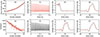Figure 8. String wire-pluck comparison. Measurement data is shown with red dots or lines and the model data is shown with a black line. (a) Theory fit to mode frequency data extracted from measurement. (b) Theory fit to Q-factor data extracted from measurement. (c) Measured wire-pluck signal. (d) Simulated wire-pluck signal. (e) Initial release stage. (f)–(h) First three sets of reflected waves.

The transversal bridge force signal obtained via simulation of only the string using a triangular initial pluck shape⁷ with x_b/L = 0.104 is plotted in Figure 8d, showing a strong resemblance to the measured pluck signal seen in Figure 8c. The corresponding initial release stages are juxtaposed in Figure 8e, and the remaining subplots compare the initial sets of reflected waves. The good waveform match confirms that the transversal vibration characteristics of the string are accurately modelled.

3.2. Comparison in the Schelleng plane

The robot arm was programmed to perform bow strokes that start from zero velocity and consist of three stages. First the bow undergoes constant acceleration over a short period, which is followed by a period of steady velocity (0.1 m/s). In the third and final stage the bow velocity is linearly decreased until the bow is back into a stationary position. Guided by findings in recent experimental research [39, 49, 50], the acceleration value was chosen in a specific range with the aim to enhance the likelihood of Helmholtz motion occurring within the steady-velocity period. During the steady-velocity stage, the signal measured with the robot load cell typically exhibited a small normal load reduction relative to the intended bowing force. For this reason, the average over the analysis window of the steady-velocity signal portion was recorded as the applied bowing force.

A total of 1600 of such bow-stroke experiments were conducted across a grid of 40 bowing positions and 40 bowing forces. Analysis of the various signals captured by the experimental apparatus indicated that the robot reliably reached the target steady-velocity value with high accuracy. However from the recorded bridge force signals it could be seen that the string was often slightly displaced from its rest position at first contact with the robot arm, meaning that the initial conditions differ per experiment and slightly deviate from what is assumed in the simulation. Further uncertainties arise from observing, for small x _b values, acceleration constants that are well below what one would expect from equation (89), which is likely due to creep [9]. Conversely, for larger x _b values some of the measured bridge force signals displayed a faster upwards rise than predicted with (89), possibly after an initial delay, which likely indicates unmodelled system compliances/inertances associated with the bow holder. Because of these uncertainties and non-idealities, the scope for a model-versus-measurement comparison of transient behaviour is somewhat limited. The focus in this section is therefore largely on assessing whether – for a specific bowing position and bowing force – the model predicts the same sustained oscillation regime in the steady-velocity part as observed in the experiment.

3.2.1. Bridge force waveforms

Figure 9 shows a selection of measured and simulated bridge force waveforms for x_b/L = 0.0874. In the left two panels, the initial transients show strong global similarities in terms of signal amplitude and type of slips that occur. The differences can mainly be seen in the finer waveform structures. The fact that the initial slips look fairly similar is a promising indication.

Figure 9. Bridge force waveforms for ten different bowing force values with the bow positioned at x b = 0.0874L. For clarity, the waveforms are offset by 3 N. From bottom to top, the bowing force values are (in N): 0.23, 0.35, 0.47, 0.65, 0.88, 1.22, 1.51, 2.10, 2.96, 4.18.

The final two panels of Figure 9 show a few periods of the steady-velocity portion of the same signals. Helmholtz motion as well as double-slip waveforms can be observed. In most cases, the model predicts the same oscillation regime as observed in the measurement, but the double-slip pattern for f_b = 0.65 N seen in the measurement is not predicted by the model. As will be seen below, this result falls within a “patchy Helmholtz region”, so the prediction failure is probably not very significant. On the other hand, the stronger ripples in the simulated waveform for f_b = 4.18 N announce an earlier transition to raucous motion, and are indicative of the model predicting a slight higher value for the maximum bowing force for which Helmholtz motion is sustained than can be inferred from the measurements.

3.2.2. Schelleng diagrams

A bird’s-eye view of the entire set of results can be provided by means of a Schelleng diagram (see Figure 10), in which regime types are plotted against relative bow-bridge distance x_b/L and bowing force f_b, both on a logarithmic scale. To assign a regime type, an automatic classification algorithm was applied to a steady-state part of each bridge force waveform. The original aim of a Schelleng diagram is to investigate the minimum and maximum bowing force that can sustain Helmholtz motion [51, 52], but here the diagrams are primarily a means of testing how well the model predicts the steady-state behaviour observed in the experiments. With that in mind, the fact that the specific bow velocity and bowing force signals differ somewhat from those applied in previous studies [51, 52], should be noted but is only of secondary importance.

Figure 10. Schelleng diagrams as measured (left) and simulated (right). The regimes are labelled as follows: Helmholtz motion (◼), double slips (*), raucous motion (+), multiple slips (×), S-motion (•), multiple flyback (▴), unclassified (•). The upper two black lines delineate the approximate Helmholtz region in the measured data, and the lower black line shows the approximate boundary between double-slip and multiple-slip motion. To aid visual comparison these lines are also added to the simulated Schelleng diagram.

The classification procedure detects six distinct regimes. These are listed with example waveforms in Figure 11. The algorithm is the same as used in a previous study [49], which was based on the methodology developed by Galluzzo [9]. One difference with [49] is that small-amplitude regimes that do not closely resemble any of the six types listed here are assigned as “unclassified”. This “none-of-the-above” category includes continuous and irregular slipping as well as regular slipping patterns featuring strongly rounded corners.

Figure 11. Example bridge force waveforms for six oscillation regimes.

The measured and simulated Schelleng diagrams are compared in Figure 10. With the chosen model parameters the Helmholtz region is reasonably well matched by the simulation, reproducing even some of the Helmholtz patchiness in the vicinity of the minimum bowing force line. The boundary between double slips and multiple slips is also similar except at very small bowing force values, while S-motion correctly occurs for x _b/L values between 0.15 and 0.2. However, S-motion is exhibited at lower bowing force values than with the measurement. This deviation is perhaps not that surprising given that whether or not any of the patterns that Raman referred “higher types of motion” [2] is triggered is highly dependent on the specific conditions. On inspection of the waveforms in this region of the Schelleng plane, the differences between measurement and simulation are often very small, just falling on either side of a classification boundary. The other main difference is that in the lower-left corner of the Schelleng plane, the simulation produces waveforms that are less easily classified than those driven by the robot arm. Overall the indications are that the match between experiment and model deteriorates at small bowing forces.

3.2.3. Further measures

The Schelleng diagram comparison in Figure 10 provides a direct sense of how well the model predicts the steady-state regime that is sustained for a given set of bowing parameters, but some detail may be obscured due to the classification coarseness. This motivates additional unpacking of the differences, here via four further measures: the mean (in N), the root mean square (RMS) about the mean (in N), the fundamental frequency (in Hz), and the power-weighted spectral centroid (in Hz), each of which can be loosely related to a perceptual attribute. That is, the mean force provides a measure of the effort required to move the bow with constant velocity v _b = 0.1 m/s in the presence of the friction force, while the RMS gives a rough indication of the amplitude of the fundamental of the tone produced. The fundamental frequency is a good estimate of the perceived pitch, and the spectral centroid provides a first indication of the tone’s brightness.

Figure 12 compares the model with the measurement in the Schelleng plane across these four measures. The vertical stripes visible in the fundamental frequency plot for the measurement (third panel in the top row) are not a feature of bowed-string dynamics but rather a reflection of the fact that the string was automatically re-tuned after each set of 40 experiments carried out for a specific bow-bridge distance. Because the system can tune to about ±0.5 Hz accuracy, these variations per Schelleng-plane column occur, alongside further small detuning ocurring across any of the sets of 40 experiments. The blue zones in both of the fundamental frequency plots indicate pitch flattening, which as expected occurs just below the maximum bowing force boundary [49, 53, 54], although not quite to the same extent. Another striking aspect is the speckledness in the plots of the RMS and spectral centroid of the measured bridge waveforms, which is not fully replicated by the model. This illustrates the sensitive dependence of bowed strings to the conditions (e.g. the material distribution of rosin accros the interfacial layer), that cannot be fully controlled in the experiments. A further anomalous feature of the measurement data is noise contamination, leading to a poor signal-to-noise ratio in the lower-left corner of the Schelleng plane, which is the main cause behind the higher spectral centroid in that region.

Figure 12. Further measures of the bridge force signal in the Schelleng plane. Top row: measurement. Bottom row: simulation. In both rows, the grey-coloured areas in each third plot indicate that the calculated fundamental frequency lies above 101 Hz in that region of the Schelleng plane, which includes all cases of raucous motion. In the fourth panel on the top row, grey-coloured areas indicate a spectral centroid larger than 1000 Hz, which occurs due to noise contamination.

Beyond these initial observations, the model largely produces very similar patterns, with one exception: the model predicts a larger mean value at the upper bowing force range. Potentially this could be an indication that the assumption of the effective thermal contact area being proportional to the bowing force breaks down in this region of the Schelleng plane. An alternative explanation is that the simplified, non-convolutional way that heat conduction has been modelled is not sufficient for accurate prediction at the upper edges of the Schelleng plane.

3.2.4. Model without the Stribeck effect

As seen in Section 2.7.2, the proposed model naturally produces rapid transitions from sticking to slipping, even for the case μ_d = μ_s, in which case there is no Stribeck effect in μ_str(v). A question then arises on whether there is a need for including a velocity-dependent curve in the expression for the friction force, which in [13] is considered as an ad-hoc modification of the original thermal model motivated purely by attempting to overcome that model’s inability to reproduce fast transitions. Hence it is of interest to assess how well the thermal elasto-plastic model can predict oscillation regimes for the special case μ_d = μ_s.

Figure 13 shows the Schelleng diagram for μ_d = μ_s, with three further friction parameters (y_a, τ_g, and b_τ) re-tuned. The match is only slightly worse than before, which suggests there may be scope for advancing the proposed model without incorporating the Stribeck effect, instead seeking to improve the predictions by adjusting other aspects (e.g. the heat balance equation).

Figure 13. Schelleng diagram as predicted by the model with μ d = μ s. The model parameters are as listed in Table 1, except for four friction parameters: μd = 1.05, ya = 0.3, τg = 35, and bτ = 0.2. As in Figure 10, for easy comparison the black lines mark the boundaries observed in the measured Schelleng diagram.

3.3. Discussion

It is worth highlighting that to obtain a decent prediction of the Helmholtz region, the friction parameters were set and adjusted by checking how the resulting bridge force waveforms visually compare to measured bridge force signals, i.e. a subset of the same data that the model output is validated against. Ideally, the parameters of a physical model are determined via independent measurements. This is relatively straightforward for the string parameters, but setting the friction parameters is much more challenging, leading to uncertainties around any set of values arrived at by tuning within physically plausible ranges.

Woodhouse and Galluzzo [13] address this calibration question by (1) forcing their model to have steady-sliding behaviour that matches the experimental results with a rosin-coated rod on a perspex wedge, and (2) deriving an additional friction curve that fits scatter data inferred from the force drop at the first slip across a large batch of measured bridge force signals. In the latter, an assumption has been made that the contact temperature (referred to as the “crossing temperature” in [13]) in all the first slips is roughly the same, regardless of the relative velocities involved; it is not clear though to what extent this actually holds. Nor is it straightforward to assume that steady-sliding experiments with rosin-coated bow on an immobilised string would yield the same steady-sliding friction curve found in [8]. Moreover, as explained in [14], for the simulation calibrated in this manner to work as planned the contact temperature has to be artificially held at the crossing temperature until the first slip, which is inconsistent with the underlying model.

In other words, this set of calibrations also leaves some uncertainty about the validity of the model and of the values of the friction parameters. As a result, for both the enhanced thermal model and the thermal elasto-plastic model it can be difficult to attribute observed discrepancies to specific model limitations. The implication is that to advance bowed-string modelling, different and better calibration experiments will likely be required.

There are however already some clues among the current findings about possible directions in which the proposed friction model will need to be further developed before it can be adopted as a reliable tool for predicting the oscillations of bowed-string instruments. These include discrepancies in the Schelleng diagram at small and large bowing forces, which appear not to be co-addressable by altering the model parameters. A plausible explanation would seem that this is due to the non-convolutional form of the heat balance equation, which will likely need refined in order to better capture the thermal dynamics, ideally still arriving at a continous-domain form that affords proving solution uniqueness; further scrutiny of the relationship between contact area and bowing force may also be warranted. The validation of any such refinements would be greatly helped if further experiments could also measure temperature at or near the frictional contact area.

The deeper general issue is that bow-string friction is in essence a multi-scale modeling problem in which the dynamics of the string is governed by behavior occuring at a length scale much smaller than its dimensions. The micro-scale behaviour is subject to various material aspects including surface roughness, contamination, and temperature; uncertainties and challenges thus typically arise around determining how the parameters of a macro-scale friction model depend on these conditions, which may vary per experiment and even during an experiment. In addition, a bowed string exhibits “twitchy” behaviour suggesting it operates at the edge of chaos, which presents further complications when attempting to conduct rigorous calibration and validation. These factors make the long-term aim of a bowed-string simulation that can accurately predict both transient behaviour and oscillation regimes a particularly challenging musical acoustics problem.

4. Conclusion

The proposed friction model incorporates two phenomena that introduce frictional hysteresis, namely thermal effects and elasto-plastic behaviour of the rosin. The thermal effects strongly influence the system dynamics during gross sliding, while explicitly modelling the rosin deformation enables transitions between sticking and slipping that are physically plausible in terms of their rapidity and smoothness. As such, the gap between thermal models and elasto-plastic models developed for bowed-string simulation has been substantially narrowed, opening up new avenues for exploring the acoustics, playability, and sound synthesis of bowed-string instruments.

The variation of the contact temperature has been modelled with a simplified heat balance equation, while the effect of the temperature on the friction coefficient was defined with a closed-form expression featuring three parameters. These two definitions were taken as the starting point for deriving a co-parameterised steady-state friction curve and Stribeck curve; the latter is required in the calculation of the friction force. The model was shown to be guaranteed passive and the equations were shown to always have a unique solution. Hence hysteresis arises naturally from the system equations in the proposed approach, which as such side-steps the need for imposing hysteresis rules.

The validity of the friction model was tested by comparing bridge force waveforms predicted by a modally-expanded bowed-string simulation with those obtained via measurement with a cello string. Using a steady-state bow velocity of 0.1 m/s, these validations were carried out across a dense range of bowing force and bow-bridge distance values. For the chosen set of friction parameters, the model was shown to provide a reasonably accurate prediction of the Helmholtz region in the Schelleng plane. Further promising findings include that the boundary between double and multiple slipping partly matches with the experimental findings and that S-motion occurs in approximately the correct region in the Schelleng diagram. The Schelleng-plane comparisons also hold up quite well in terms of further measures such as the RMS and the spectral centroid. In addition it was shown that the friction parameters can be slightly adjusted to render a decent Schelleng diagram match for the case of defining the steady-state coefficient of friction as decreasing with temperature but not with velocity; this special case represents an alternative approach to addressing the main shortcoming of the original thermal model as identified in [13].

Further insights into steady-state behaviour can be obtained by conducting similar comparisons for different steady-state bow velocities. More pertinently, a fuller understanding requires investigating the model’s ability to predict transients, which is usually assessed by comparing Guettler diagrams [12, 14]; work in this direction stands to be reported in [55]. In addition, it would be helpful to conduct parametric studies to gain further insight into sensitivity of the oscillatory behaviour to value changes in each of the friction parameters. However the authors’ expectation is that advancing the friction model to better capture the entire dynamics will also require new experiments for improved calibration of the friction parameters.

Acknowledgments

The first author is grateful for the generous insight offered by Prof Jim Woodhouse during several informal conversations on the topic of bowed-string acoustics. We also thank Fan Tao and Tom Nania (both at D’Addario & Co.) for providing the D’Addario strings for the experiments.

Funding

This research was funded in whole or in part by the Austrian Science Fund (FWF) [10.55776/P34852].

Conicts of interest

The authors declare that they have no conflicts of interest in relation to this article.

Data availability statement

Data are available on request from the authors. The measurement data is available in Zenodo, under the reference https://zenodo.org/records/17782538 (string type B, tension T2).

References

Appendix A

Assuming a circular contact area of radius r_c, the heat balance equation for a point-bow is given in [8] as

$$\begin{array}{cc}\hfill f_{\mathrm{b}}{\mu }_{\mathsf{ss}}(v)v& ={\rho }_{\mathsf{r}}{A}_{\mathrm{c}}{\delta }_{\mathsf{r}}{c}_{\mathsf{r}}{d}_t\tau +v{r}_{\mathrm{c}}{\delta }_{\mathsf{r}}{\rho }_{\mathsf{r}}{c}_{\mathsf{r}}\tau \hfill \\ \hfill & +{\int }_{-\infty }^{t}g(t-t^{\prime })\tau (t^{\prime })\mathrm{d}{t}^{\prime },\hfill \end{array}$$(A.1)

where g(t)=g ₁(t)+g ₂(t) is a sum of two Green’s functions, associated with heat conduction into the stationary surface (string) and the moving surface (bow hair), respectively. The first term on the right-hand side represents heat absorption, and the second term models advection. Under steady sliding, this becomes

$$\begin{array}{c}\hfill f_{\mathrm{b}}{\mu }_{\mathsf{ss}}(v)v=v{r}_{\mathrm{c}}{\delta }_{\mathsf{r}}{\rho }_{\mathsf{r}}{c}_{\mathsf{r}}\tau +\tau A_{\mathrm{c}}{\kappa }_{\mathsf{r}}\sqrt{\frac{3v}{8r_{\mathrm{c}}{D}_{\mathsf{r}}}},\end{array}$$(A.2)

where the square-root originates from truncating g ₂(t) to account for the bow hair representing a moving surface, while the conduction into the string vanishes due to the reduced dimensionality of the employed heat equation (e.g. radiative loss is neglected)[8]. This means that this model predicts that there is zero heat flux into the string under steady-state conditions.

For the point-bow version of the model proposed in the current study, spatially integrating (28) over ℬ amounts to multiplying with W _b. If the formulas in (23)–(25) are applied, the heat balance for steady-state friction with v >  0 can then be written as

$$\begin{array}{c}\hfill f_{\mathrm{b}}{\mu }_{\mathsf{ss}}(v)v=\tau A_{\mathrm{c}}[{\kappa }_{\mathsf{r}}\sqrt{\frac{2v}{\pi l_{\mathrm{c}}{D}_{\mathsf{r}}}}+\frac{{\kappa }_{\mathrm{e}}}{l_{\mathrm{e}}}],\end{array}$$(A.3)

where the proportional relationship f _b = A _c𝒯_b/r was used. In our model, the logical replacement for “average transit time” 8r _c/[3π v] that holds for a circular contact area as assumed in [8] is l _c/[2v]. Taking this replacement into account, equation (A.3) mirrors (A.2) but with the advection term replaced by velocity-independent conduction. Since both terms are typically far smaller than the velocity-dependent conduction, the friction model can be said to be qualitatively similar to the model proposed in [8] in terms of steady-state behaviour. More generally, when applying (23)–(25) to define the heat-balance coefficients, equation (22) can be written as

$$\begin{array}{c}\hfill {\mathcal{Q}}_{\mathrm{f}}=\stackrel{{\displaystyle {\rho }_{\mathsf{r}}^{\prime }}}{\overbrace{{\rho }_{\mathsf{r}}{\delta }_{\mathsf{r}}{l}_{\mathrm{c}}}}{c}_{\mathsf{r}}{\partial }_t\tau +{\kappa }_{\mathsf{r}}\tau \sqrt{\frac{2l_{\mathrm{c}}|v|}{\pi D_{\mathsf{r}}}}+{\kappa }_{\mathrm{e}}\tau \frac{l_{\mathrm{c}}}{l_{\mathrm{e}}},\end{array}$$(A.4)

where ρ^′_r is the mass per unit length of the rosin within the contact layer.

Appendix B

Writing (28) as

$$\begin{array}{c}\hfill [b_{\tau }\sqrt{v/F_{\mathrm{b}}}+c_{\tau }]\tau ={\mu }_{\mathsf{ss}}(\tau )v,\end{array}$$(B.1)

we may find v directly from τ as

$$\begin{array}{c}\hfill v=\frac{1}{F_{\mathrm{b}}}{\left[\frac{b_{\tau }\tau +\sqrt{b_{\tau }^2{\tau }^2+4c_{\tau }\tau {\mu }_{\mathsf{ss}}(\tau )F_{\mathrm{b}}}}{2{\mu }_{\mathsf{ss}}(\tau )}\right]}^2·\end{array}$$(B.2)

The other way around is more difficult. We may write (B.1) as a nonlinear equation in τ:

$$\begin{array}{c}\hfill f_{\mathrm{n}\mathrm{l}}(\tau )={\mu }_{\mathsf{ss}}(\tau )v-[b_{\tau }\sqrt{v/F_{\mathrm{b}}}+c_{\tau }]\tau =0,\end{array}$$(B.3)

which for a given v can be solved with Newton’s method. The derivate is ${\partial }_{\tau }{f}_{\mathrm{n}\mathrm{l}}={\partial }_{\tau }{\mu }_{\mathsf{ss}}-[b_{\tau }\sqrt{v/F_{\mathrm{b}}}+c_{\tau }]$, where

$$\begin{array}{c}\hfill {\partial }_{\tau }{\mu }_{\mathsf{ss}}=\frac{[{\mu }_{\mathrm{d}}{y}_{\mathrm{a}}-{\mu }_{\mathrm{s}}]{[\tau /{\tau }_{\mathrm{g}}]}^{\xi -1}}{{\tau }_{\mathrm{g}}^{\xi }\{1+{[\tau /{\tau }_{\mathrm{g}}]}^{\xi }\}}\le 0.\end{array}$$(B.4)

References

- H. von Helmholtz: On the Sensations of Tone as a Physiological Basis for the Theory of Music. Reprinted by Dover, New York, 1954, p. 1862. [Google Scholar]
- C.V. Raman: On the mechanical theory of the vibrations of bowed strings and of musical instruments of the violin family, with experimental verification of the results. Part I. Indian Association for the Cultivation of Science Bulletin 15 (1918) 1–158. [Google Scholar]
- M.E. McIntyre, R.T. Schumacher, J. Woodhouse: New results on the bowed string. Catgut Acoustical Society Newsletter 28 (1977) 27–31. [Google Scholar]
- M.E. McIntyre, J. Woodhouse: On the fundamentals of bowed string dynamics. Acustica 43, 2 (1979) 93–109. [Google Scholar]
- M.E. McIntyre, R.T. Schumacher, J. Woodhouse: On the oscillations of musical instruments. The Journal of the Acoustical Society of America 74, 5 (1983) 1325–1345. [CrossRef] [Google Scholar]
- H. Olsson: Control systems with friction. Ph.D. thesis, Lund Institute of Technology (LTH), 1996. [Google Scholar]
- H. Lazarus: Die Behandlung der selbsterregten Kippschwingungen der gestrichenen Saite mit Hilfe der endlichen Laplacetransformation. Ph.D. thesis, Technical University of Berlin, 1972. [Google Scholar]
- J. Smith, J. Woodhouse: The tribology of rosin. Journal of the Mechanics and Physics of Solids 48 (2000) 1633–1681. [CrossRef] [Google Scholar]
- P. Galluzzo: On the playability of stringed instruments. Ph.D. thesis, Trinity College, University of Cambridge, 2004. [Google Scholar]
- J. Woodhouse: Bowed string simulation using a thermal friction model. Acta Acustica united with Acustica 89 (2003) 355–368. [Google Scholar]
- J. Woodhouse: The acoustics of the violin: a review. Reports on Progress in Physics 77, 11 (2014) 115901. [CrossRef] [PubMed] [Google Scholar]
- P. Galluzzo, J. Woodhouse, H. Mansour: Assessing friction laws for simulating bowed-string motion. Acta Acustica united with Acustica 103, 6 (2017) 1080–1099. [CrossRef] [Google Scholar]
- J. Woodhouse, P. Galluzzo: Enhanced tribological modelling of violin rosin. Tribology Letters 73, 128 (2025) 12. [Google Scholar]
- J. Woodhouse: The science of musical instruments, 2026. https://euphonics.org [Accessed: 2026-01-12]. [Google Scholar]
- J.R. Rice, N. Lapusta, K. Ranjith: Rate and state dependent friction and the stability of sliding between elastically deformable solids. Journal of the Mechanics and Physics of Solids 49, 9 (2001) 1865–1898. [Google Scholar]
- A. Champneys, P.L. Várkonyi: The Painlevé paradox in contact mechanics. IMA Journal of Applied Mathematics 81 (2016) 538–588. [Google Scholar]
- S.J. Hogan, K.U. Kristiansen: On the regularization of impact without collision: the Painlevé paradox and compliance. Proceedings of the Royal Society A: Mathematical, Physical and Engineering Sciences 473, 2202 (2017). [Google Scholar]
- F.G. Friedlander: On the oscillations of a bowed string. Mathematical Proceedings of the Cambridge Philosophical Society 49 (1953) 516–530. [CrossRef] [Google Scholar]
- R.T. Schumacher, S. Garoff, J. Woodhouse: Probing the physics of slip-stick friction using a bowed string. Journal of Adhesion 81 (2007) 723–750. [Google Scholar]
- R.T. Schumacher, J. Woodhouse: The transient behaviour of models of bowed-string motion. Chaos 5, 3 (1994) 509–523. [Google Scholar]
- S. Serafin, F. Avanzini, D. Rocchesso: Bowed string simulations using an elasto-plastic friction model, in: Proceedings of the Stockholm Music Accoustics Conference, 2003. [Google Scholar]
- S. Willemsen, S. Bilbao, S. Serafin: Real-time implementation of an elasto-plastic friction model applied to stiff strings using finite-difference schemes, in: Proceedings of the International Conference on Digital Audio Effects, 2019, pp. 40–46. [Google Scholar]
- E. Matusiak, V. Chatziioannou: A comparison of friction models for bow-string interaction based on experimental measurements, in: Proceedings of International Symposium on Musical Acoustics, Vol. 6, 2023, pp. 9–16. [Google Scholar]
- P. Dupont, B. Armstrong, V. Hayward: Elasto-plastic friction model: contact compliance and stiction, in: Proceedings of 2000 ACC. IEEE, Chicago, 2000. [Google Scholar]
- P. Dupont, V. Hayward, B. Armstrong, F. Altpeter: Single state elasto-plastic friction models. IEEE Transactions on Automatic Control 47, 5 (2002) 787–792. [Google Scholar]
- C. Canudas de Wit, H. Olsson, K. Åström, P. Lischinsky: A new model for control of systems with friction. IEEE Transactions on Automatic Control 40, 3 (1995) 419–425. [Google Scholar]
- E. Matusiak, V. Chatziioannou: Elasto-plastic friction modeling toward reconstructing measured bowed-string transients. The Journal of the Acoustical Society of America 156, 2 (2024) 1135–1147. [Google Scholar]
- E. Matusiak, V. Chatziioannou, M. van Walstijn: Numerical modelling of elasto-plastic friction in bow-string interaction with guaranteed passivity. Frontiers in Signal Processing 5 (2025). [Google Scholar]
- E. Matusiak, V. Chatziioannou, M. van Walstijn: A refined bow-string interaction model considering hysteresis. Proceedings of Meetings on Acoustics 58, 1 (2025) 10. [Google Scholar]
- M. Demoucron: On the control of virtual violins physical modelling and control of bowed string instruments. Ph.D. thesis, Royal Institute of Technology, Stockholm, 2008. [Google Scholar]
- O.J.P.F. Inácio: A modal method for the simulation of nonlinear dynamical systems with application to bowed musical instruments. Ph.D. thesis, University of Southampton, 2008. [Google Scholar]
- R. Pitteroff, J. Woodhouse: Mechanics of the contact area between a violin bow and a string. Part I: reflection and transmission behaviour. Acta Acustica united with Acustica 84 (1998) 543–562. [Google Scholar]
- C. Desvages, S. Bilbao, M. Ducceschi: Improved frequency-dependent damping for time domain modelling of linear string vibration, in: Proceedings of the International Congress on Acoustics Buenos Aires, Argentina, 2016. [Google Scholar]
- K. Johanastrom, C. Canudas de Wit: Revisiting the LuGre friction model. IEEE Control Systems Magazine 28, 6 (2008) 101–114. [Google Scholar]
- P. Dahl: A solid friction model. Technical report, The Aerospace Corporation, El Segundo, CA, 1968. [Google Scholar]
- C. Canudas de Wit, P. Tsiotras: Dynamic tire friction models for vehicle traction control, in: Proceedings of the 38th IEEE Conference on Decision and Control, Vol. 4, 1999, pp. 3746–3751. [Google Scholar]
- F. Marques, Ł. Woliński, M. Wojtyra, P. Flores, H.M. Lankarani: An investigation of a novel LuGre-based friction force model. Mechanism and Machine Theory 166 (2021) 104493. [Google Scholar]
- J. Koopman, D. Jeltsema, M. Verhaegen: Port-Hamiltonian description and analysis of the LuGre friction model. Simulation Modelling Practice and Theory 19, 3 (2011) 959–968. [Google Scholar]
- A. Lampis, A. Mayer, V. Chatziioannou: Assessing playability limits of bowed-string transients using experimental measurements. Acta Acustica 8 (2024) 44. [Google Scholar]
- F.P. Bowden, D. Tabor: The Friction and Lubrication of Solids. Clarendon Press, Oxford, 1950, re-published by Oxford University Press in 2001. [Google Scholar]
- J.A. Greenwood, J.B.P. Williamson: Contact of nominally flat surfaces. Proceedings of the Royal Society of London. A. Mathematical and Physical Sciences 295, 1442 (1966) 300–319. [Google Scholar]
- F. Ablitzer, N. Dauchez, J.P. Dalmont: A predictive model for the adjustment of violin bows. Acta Acustica united with Acustica 98, 4 (2012) 640–650. [Google Scholar]
- C. Valette: Mechanics of vibrating strings, in: A. Hirschberg, J. Kergomard, G. Weinreich (Eds.). Mechanics of Musical Instruments, 1995, pp. 115–183. [Google Scholar]
- J. Woodhouse: Plucked guitar transients: comparison of measurements and synthesis. Acta Acustica united with Acustica 90 (2004) 945–965. [Google Scholar]
- J. Woodhouse, A.R. Loach: Torsional behaviour of cello strings. Acta Acustica united with Acustica 85 (1999) 734–740. [Google Scholar]
- L. Barreira, C. Valls: Ordinary Differential Equations: Qualitative Theory. American Mathematical Society, 2012. [Google Scholar]
- J.C. Schelleng: The bowed string and the player. Journal of the Acoustical Society of America 53 (1973) 26–41. [CrossRef] [Google Scholar]
- A. Mayer, A. Lampis: A versatile monochord setup: an industrial robotic arm as bowing and plucking device. Technical report, University of Music and Performing Arts Vienna, 2024. [Google Scholar]
- A. Lampis, V. Chatziioannou, G. Scavone: Experimental analysis of cello string types: influence on playability and tonal characteristics using Schelleng diagrams, in: International Symposium on Music and Room Acoustics, 2025, p. 035013. [Google Scholar]
- A. Lampis, A. Mayer, V. Chatziioannou: An experimental approach for comparing the influence of cello string type on bowed attack response. JASA Express Letters 4 (2024) 113201. [Google Scholar]
- E. Schoonderwaldt, K. Guettler, A. Askenfelt: An empirical investigation of bow-force limits in the Schelleng diagram. Acta Acustica united with Acustica 94 (2008) 604–622. [CrossRef] [Google Scholar]
- P. Galluzzo, J. Woodhouse: High-performance bowing machine tests of bowed-string transients. Acta Acustica united with Acustica 100 (2014) 139–153. [CrossRef] [Google Scholar]
- E. Schoonderwaldt: The violinist’s sound palette: spectral centroid, pitch flattening and anomalous low frequencies. Acta Acustica united with Acustica 95 (2009) 901–914. [CrossRef] [Google Scholar]
- H. Mansour, J. Woodhouse, G. Scavone: Enhanced wave-based modelling of musical strings. Part 2: bowed strings. Acta Acustica united with Acustica 102 (2016) 1094–1107. [Google Scholar]
- V. Chatziioannou, M. van Walstijn, A. Lampis: Simulating bow-string transients using a thermal elasto-plastic friction model, in: The International Symposium on Musical Acoustics, Helsinki, Finland, 2026. [Google Scholar]