| Issue |
Acta Acust.
Volume 9, 2025
Topical Issue - Musical Acoustics: Latest Advances in Analytical, Numerical and Experimental Methods Tackling Complex Phenomena in Musical Instruments
|
|
|---|---|---|
| Article Number | 4 | |
| Number of page(s) | 22 | |
| DOI | https://doi.org/10.1051/aacus/2024067 | |
| Published online | 13 January 2025 | |
Scientific Article
An experimental study on the perception of violin bow mass distribution
1
Sorbonne Université, CNRS, Institut Jean Le Rond d’Alembert, 75005 Paris, France
2
Bow Maker, Nantes, France
3
Laboratoire d’Acoustique de l’Université du Mans (LAUM), UMR 6613, Institut d’Acoustique – Graduate School (IA-GS), CNRS, Le Mans Université, 72085 Le Mans, France
* Corresponding author: This email address is being protected from spambots. You need JavaScript enabled to view it.
Received:
4
April
2024
Accepted:
28
September
2024
Abstract
The goal of this study is to investigate the perception of different bow mass distributions using an experimental violin bow. The position of the centre of mass and the moment of inertia were independently modified through five distinct mass configurations, which were tested by multiple violinists. Various perceptual tests, including three discrimination tests and a free evaluation test, were conducted. Concepts from Signal Detection Theory were used to calculate a representative sensitivity value, considering participants’ sureness in their responses to discrimination tests. Results indicate that participants were sensitive to a substantial variation (10%) in the position of the centre of mass when holding the bow in the air versus during playing, though they did not seem to perceive minor changes (4%) significantly. Conversely, participants exhibited sensitivity to both minor (4%) and substantial (12%) variations in the moment of inertia while playing, suggesting a heightened awareness of even slight modifications in this parameter. Furthermore, the free evaluation test revealed that the perceived bow weight was influenced by both parameters, while the quality of bouncing bow strokes appeared to be more influenced by the moment of inertia.
Key words: Violin bow / Bow making / Perception / Discrimination / Human-instrument interaction
© The Author(s), Published by EDP Sciences, 2025
 This is an Open Access article distributed under the terms of the Creative Commons Attribution License (https://creativecommons.org/licenses/by/4.0), which permits unrestricted use, distribution, and reproduction in any medium, provided the original work is properly cited.
1 Introduction
Bows primarily consist of two parts: the hair that comes into contact with the strings, traditionally made from horsehair to which rosin is added to enhance adhesion, and a wooden stick (Fig. 1), typically made of pernambuco wood and whose main function is to maintain the tension of the hair. This study focuses on the latter. When playing, violinists hold the bow with their right hand and control, among others, the following key bowing parameters: speed, position along the string, and vertical force applied to the strings. These different parameters trigger various vibrational regimes of the strings, which are then transmitted through the bridge to the corpus (soundbox) and ultimately into the air, resulting in distinct sounds [1]. Violinists master the control of these bowing parameters to achieve the desired sound in line with their interpretive intentions.
 |
Figure 1 Overview of the violin bow main parts, without hair. |
Despite being an essential element for most violinists, the bow has not received the same level of attention from researchers as the violin until the latter part of the twentieth century. Just a few studies have explored violinists’ perception of bows. One of the earlier attempts to unveil the relationship between bow mechanical properties and their perceived qualities was conducted by Bissinger in 1995 [2]. He conducted modal analysis and bounce tests on eight violin bows, followed by evaluations by an expert violinist. The bows with the highest modal damping were perceived as “squishy” and “soft”, while those with lower damping were associated with an “out-of-control feeling to spiccato and ricochet” (two bowing techniques involving bouncing the bow on the strings). Bows classified as “excellent spiccato bows” fell in between. A few years later, Caussé et al. [3] conducted a dissimilarity test involving twelve expert violinists using a set of seven carbon fiber composite bows and a pernambuco bow. They could not establish correlations between quality criteria and physical properties such as mass, centre of gravity, stiffness, or hair tension. However, they identified three critical playing properties that were consistently important to all violinists: balance, flexibility, and responsiveness. Ablitzer et al. [4, 5] delved into the influence of camber (i.e., the curvature of the stick) on bow playing qualities. They used three bows with different camber levels, which were characterised and tested by two expert violinists. They found that variations in hair tension, determined by camber at a given hair-stick distance, influenced the perceived attack transients and reactivity of the bow (i.e. the ability of the bow to respond to the violinists’ actions). Bow maker Joseph Regh recently published the results of a lifelong study on bows [6]. Over the years, he asked 10 professional violinists to play and rate a set of 75 bows with varying physical properties. Three properties emerged as key determinants of perceived bow quality: hair tension, moment of inertia, total mass, and stick stiffness. The 12 most preferred bows, compared to the 12 least liked ones, were significantly heavier by 3.6 g (62.2 g vs. 58.6 g respectively), with a moment of inertia around the thumb position of 0.31 gm2 higher (5.49 gm2 vs. 5.18 gm2 respectively), with a significantly higher hair tension for the same hair-stick distance and with a higher bending stiffness of the stick.
None of the aforementioned studies have specifically investigated how mass distribution influences bow quality. Moreover, most of these studies employed different bows with their unique characteristics (wood, hair, mass distribution or total weight), which makes it difficult to isolate the impact of each characteristic on perceived qualities. In 2017, an experiment led by Tomezzoli et al. [7] at the University of Montreal explored the influence of bow camber and mass distribution on violinists’ preferences. In this study, a single 62 g bow was used, with various masses added at different locations (tip and frog, 1 and/or 2 g). In general, the additional masses at the tip and/or frog affected negatively violinists’ ratings, likely due to significant alterations in bow mechanical properties such as the centre of mass position and the moment of inertia. However, adding 2 g to both the tip and frog brings the total weight closer to that of a viola bow (70 g) rather than a standard violin bow (60 g) [8], quite far from what violinists are used to play with.
Bow mass distribution is primarily determined by the geometry and density of the stick, but it can also be influenced by the mass of elements added after crafting. For instance, elements like the tip plate or the winding near the frog can vary in mass, thus changing the value of both the first and second moments of mass of the whole bow. In contemporary bow making, these components can be made from materials of different densities, offering the flexibility to modify the mass distribution of the entire bow after the stick is completed. Conversely, reducing mass of a bow by tapering the stick (i.e. removing wood, generally with a hand plane) can potentially jeopardise its structural integrity once the bow is made. This is not a viable option for modifying historical or high-quality bows.
A recent study [9] has shown that even for a well-trained audience (luthiers and violinists), differentiating between a violin and a viola bow based solely on the perceived sound is very challenging, if not impossible. Conversely, violinists seem to discern the differences between various bows when playing with them.
Our study follows a methodology akin to that employed by Tomezzoli et al. [7]: we explore how violinists perceive different mass distributions of a bow when they use it, by adding masses to a single modern bow’s stick. However, we used a specially designed bow that is lighter than the standard. This ensures that the tested bows’ weight is approximately 60 g – the established standard for violin bows [8] – regardless of the specific arrangement of the added masses. Our approach aims to replicate conditions closely resembling a violinist’s experience when assessing different bows, in order to analyse their sensitivity to such changes.
The present paper is structured as follows. First, some hypotheses of how changes in both the centre of mass and the moment of inertia may affect the violinist-bow interaction are given in Section 2. The experimental bow is then presented in Section 3, alongside with the different mass distributions and how the mechanical properties of interest are measured. In Sections 4 and 5 the two experiments done with violinists are explained with their respective results. Finally, the results are discussed in Section 6.
2 Influence of bow mass distribution on the fingers-bow interaction
In this section, we propose some simple physical models of the interaction between the violinist and the bow in different situations, specifically focusing on finger forces. We analyse the effect of bow mass distribution on this interaction, focusing on two mechanical properties: the horizontal position of the centre of mass and the moment of inertia. The physics discussed here have motivated the two perceptual studies presented in Sections 4 and 5, which form the main focus of this article.
We will refer to the forces that are applied by the violinist on the bow as “finger forces”. A more complex biomechanical analysis including other body parts involved in the bowing movement is beyond the scope of this paper.
This section is structured as follows. First, we explore how recent violin treatises describe the proper manipulation of the bow by the violinist to control its vertical action on the string, which inspired the modelling of the fingers-bow interaction. Then, we analyse the role of the position of the centre of mass in two situations: holding the bow horizontally in the air and bowing the string with a uniform force. Finally, we examine how the moment of inertia influences the interaction between the fingers and the bow in two additional scenarios, where the bow rotates around a pivot point: shaking the bow in the air and bouncing it on the string.
2.1 Modelling the fingers-bow interaction based on modern violin treatises
During a performance, the bow can be manipulated in numerous ways, limited only by the creativity of the composer or performer. In Western classical music specifically, there are various bow strokes that require specific motion patterns [10, 11]. However, in this study, we focus only on the vertical motion of the bow and on the forces that act in this direction. This vertical motion refers to the movement that controls the force applied to or released from the strings in a direction approximately normal to the top plate of the violin (depending on the string). Conversely, horizontal motion refers to the movement of the bow across the string.
A dilemma arises when modelling how violinists manipulate the bow to achieve this motion. Using a single individual’s technique to create a fingers-bow interaction model can lead to inaccuracies, as each violinist’s technique could be influenced by their experience, training, and physical constitution. Fortunately, violin treatises written over the centuries provide valuable insights into playing techniques. The international recognition of works by Capet [10] and Galamian [11] in the twentieth century offer a reliable basis for inspiring a simple model of the fingers-bow interaction [12, 13].
In his treatise on superior bow technique [10], Capet makes a systematic analysis of the role of each finger in the vertical movement of the bow. He emphasises the alternating forces of the index and little fingers, which enable the rotation of the bow around the pivot point formed by the thumb and middle finger (see Fig. 2). Galamian, in his treatise on violin playing and teaching [11], describes the physical motions of the fingers, hand and forearm in different bowing techniques. He analyses the vertical motion of the bow similarly to Capet, and highlights the importance of this gesture to control the force on the string.
 |
Figure 2 Detail of the role of the fingers. Left: the thumb and middle finger grip, creating a pivot point; top right: the little finger lifts the bow from the string; bottom right: the index finger presses the bow onto the string. Redrawn from Principles of violin playing and teaching (1st edn., p. 46 and 49) by I. Galamian, 1962, Prentice Hall [11]. |
In summary, from these treatises we conclude that the bow should be held with the thumb placed below the stick, touching both the stick and the part of the frog in contact with the stick that is closest to the hair. The middle finger surrounds the stick and opposes the thumb, creating a finger grip that serves as the fulcrum for balancing the bow. The ring finger falls naturally on the side of the frog, with minimal interaction with the stick for the vertical movement. Finally, the index and little fingers rest on the stick, enabling the double-leverage mechanism around the pivot point formed by the thumb and middle finger, as depicted in Figure 2. Other studies [14, 15] have proposed similar models for the interaction between the fingers and the bow to achieve vertical motion. We assume that the variability in bowing technique among players does not deviate significantly from this description.
Our model of the fingers-bow interaction is two-dimensional, so we made several simplifications. Although the bow is usually tilted across its longitudinal axis to a certain angle when playing, we assume that the bow is never tilted, meaning that the plane that contains both hair and stick is always normal to the string. Let us also consider that, when bowing the string, the bow is always drawn in a plane horizontal to the ground, so that the weight force is perpendicular to the stick. Additionally, all the distances of interest of our model are measured from the position of the pivot point formed by the thumb and middle finger. Finally, the selected axis for calculating the moment of inertia of the bow is aligned with this pivot point, oriented perpendicular to the plane containing both the hair and the stick.
2.2 Influence of the horizontal position of the centre of mass on the fingers-bow interaction
Let us present two scenarios where the centre of mass may influence how the violinist controls the bow. These scenarios do not involve vertical motion of the bow, only vertical forces on the stick. Rather than analyzing every situation that could lead to the perception of variations in the centre of mass, we have focused on two simple cases where we believe sensitivity to such changes is highest: holding the bow horizontally and bowing the string horizontally with uniform force. All the distances presented in this section are given with respect to the pivot point formed by the thumb and middle finger.
The forces exerted by the index and little fingers on the stick produce torques in opposite directions. Consequently, it is possible to achieve the same net torque with different combinations of these forces. In our model, we assume that the net torque applied by the fingers of an expert violinist on the bow is achieved with the least effort (as in [14]). The least effort solution hypothesises that there are no mechanically inefficient movements, such as cocontractions (i.e. muscles fighting against each other without resulting in any net movement [16]). This involves applying force with either the index finger or the little finger, but not both simultaneously.
2.2.1 Holding the bow horizontally in the air
Given a total bow mass, the variation in the position of the centre of mass could be perceived by the violinist through the forces they would need to apply with their fingers when holding the bow in the air. To perceive such changes, the orientation of the stick with respect to gravity is important: if the bow were held vertically, gravity would act in the longitudinal direction of the stick, and no difference would be perceived unless the total mass changes. The largest difference would be felt when the bow is held horizontally, since the moment of the weight to be compensated with the fingers is maximum for this orientation. The solution that requires the least effort to keep the bow in such a position involves using only the little finger.
To keep the bow horizontal, a rotational static equilibrium is achieved (see Fig. 3a), with the force of the little finger FL and the distance between the pivot point and the centre of mass xCM linked by a linear relationship:
 (1)where the slope is the ratio between bow’s weight Wbow and the position of the little finger with respect to the pivot point xL. From this equation we can therefore hypothesise that a variation in the position of the centre of mass could be perceived through a change in the force that the little finger needs to exert on the stick to keep it horizontal. From the slope of this relationship, we deduce that a modification in the centre of mass position would be more noticeable in heavier bows or if the little finger is positioned closer to the pivot point.
 |
Figure 3 Vertical forces acting on the bow in three different scenarios where the bow remains horizontal. (a) Holding the bow horizontally in the air. (b) Bowing the string close to the frog (0 ≤ xS < xeq). (c) Bowing the string close to the tip (xeq ≤ xS < L). |
2.2.2 Bowing the string horizontally with uniform force on the string
In a playing situation the bow is supported from below by both the thumb and the string, represented by the forces FT and Fs respectively in Figure 3. Although bow kinematics is complex [17], let us suppose, as a first approximation, that the string is bowed horizontally, which is approximately the case for G and D strings. The bow’s weight points in a direction perpendicular to the stick, as well as the vertical force applied on the string, which is the opposite of the reaction force of the string on the bow FS (Figures 3b and 3c). This vertical force FS influences, among other sound characteristics, the length of attack transients [18], and is controlled by the forces applied by the index and little fingers (respectively FI and FL) [11].
As a first approximation, let us assume that neither the stick, the hair, nor the string deflects under vertical forces. If no force is applied by the little or index fingers, the only contribution to the force on the string FS is the weight of the bow. From rotational equilibrium, we would have:
 (2)which results in a very high force FS when the hair-string contact is close to the frog (small xS) versus a low force if the contact is close to the tip (large xS). This is illustrated in Figure 4a. To modify this effect and achieve a uniform force, violinists need to press the stick either with their index or little fingers depending on the position of the string with respect to the thumb xS. This adjustment also depends on the position of the bow’s centre of mass and its weight. However, the variations in these parameters between two bows are typically not as significant as the variation of xS during a stroke.
 |
Figure 4 Resulting force on the string during a stroke with two different finger-bow interactions. The mechanical properties of the bow and the distances of the fingers to the pivot point are assumed to be as follows: mbow = 60 g, xCM = 20 cm, xI = 6.3 cm, xL = 5.6 cm. (a) Resulting force on the string when the index and little finger forces are null. (b) Finger forces required to obtain a uniform force on the string of 1 N, as presented in equation (3). |
The rotational static equilibrium of the bow is therefore given by the balance of finger forces, weight and the reaction force of the string on the bow:
 (3)where xI is the position of the index finger with respect to the thumb, L is the total hair length and xeq = xCMWbow/FS denotes the equilibrium position of the bow on the string where the force exerted by the bow’s weight on the string (as described by Eq. (2)) matches the required force. In this position, no additional force needs to be applied or removed by the index or little fingers, and marks the transition from pressing with the little finger to pressing with the index during a down-bow stroke (vice versa for an up-bow stroke), in order to ensure a uniform force on the string. In certain situations, such as when the required force on the string FS is very low, it is possible for the equilibrium position xeq to fall beyond the tip of the bow. In this case, the violinist would need to counteract the effect of the bow’s weight on FS along the entire length of the hair. As a result, only the little finger’s action would be necessary to achieve the desired force on the string. The transition between little finger and index finger forces to produce a typical uniform force of 1 N on the string (as per [19]) is represented in Figure 4b.
For higher-pitched strings (A and, above all, E), the motion of the bow closely aligns with the direction of gravity. When playing on these strings, the contribution of the bow’s weight to the force applied on the string is much lower, if not negligible. Consequently, the position of the centre of mass would not significantly affect the finger forces needed to press the string.
2.3 Influence of the moment of inertia on the fingers-bow interaction
Let us now analyse the interaction between the fingers and the bow when the bow’s rotational acceleration around the pivot point is not null. This is the case for some bow strokes like spiccato or sautillé, but also when the violinist grabs the bow and shakes it in the air, with or without a musical motivation. In this section, we will analyse these two simple cases: first the rotation of the bow around the pivot point formed by the thumb and the middle finger without contact of the string, which we will refer to as “shaking the bow”; and then the bouncing of the bow on the string.
2.3.1 Shaking the bow in the air
Let’s first consider the simpler case of shaking the bow in the air, where the player rotates the bow around the pivot point (Fig. 5a). As stated by Newton’s second law for rotation, the torque exerted by both weight and the finger forces on the bow equals the moment of inertia I times the angular acceleration  :
:
 (4)
(4)
 |
Figure 5 Vertical forces and motion of the bow in two different cases where the bow is rotated around the pivot point. (a) Shaking the bow up and down in the air. (b) Bouncing “naturally”, i.e. without any interaction of the fingers except keeping the pivot point fixed (little and index finger forces equal to zero). |
Note that, in line with the least effort principle, we assume that players only exert force either with the index or the little finger, i.e. always one of the two is equal to zero. If the angular momentum of the bow changes ( ), its rotational energy is modified over time. The net work of the forces acting on the bow – that is, finger forces and weight – is equal to the change in this energy, which is proportional to the moment of inertia. Consequently, when dealing with a bow with higher moment of inertia, finger forces must exert more work to rotate it, which could potentially be perceived by simply shaking the bow’s tip up and down in the air.
2.3.2 Bouncing the bow on the string
When playing, bow strokes like spiccato or ricochet, which imply a bouncing motion on the string, could be affected by the moment of inertia. This behaviour also entails a rotation around the pivot point fixed at the thumb position, and has already been described in literature [15, 20]. Previous studies on the perception of bow qualities [21, 22] have observed that violinists describe the bows as having a sweet spot where the bow bounces “naturally”. Here, as a first approximation, we will consider that this bounce occurs with minimal interaction from the fingers on the stick, i.e., with no index and little finger forces (see Fig. 5b).
While in this kind of strokes the bow moves both horizontally (to bow the string) and vertically (bouncing motion), let us initially assume that it only bounces on the string without any horizontal movement. This bouncing motion involves two phases: one where the bow is in contact with the string and another where it lifts off the string [11].
Let us first focus on the phase when the bow is in contact with the string. During this phase, the forces acting on the bow are its weight and the force from the string FS. Let us assume that, for small changes in the bow’s inclination (given by angle θ, as shown in Fig. 5b), FS remains perpendicular to the stick. This implies that the direction of FS is not affected by the angle θ, but its magnitude is. As indicated in the figure, FS increases with negative values of θ, corresponding to the bow exerting force on the string. Conversely, as θ approaches zero, FS decreases, and when θ becomes positive, the bow lifts off the string and FS becomes null.
Under this configuration, Newton’s second law for rotation yields:

The rotation movement during this bounce entails a very short range of angles, making it possible to apply the small angle approximation (cos(θ) ≈ 1). Thus, we can consider the weight force to be constant during this phase. The only element on the left side of the equation that is angle-dependent would then be the reaction force of the string FS. Let us also assume that neither the string nor the stick deflects under vertical forces, but the hair may. This rigid stick, quasi-static bow model was proposed by Askenfelt [15], who used it to estimate the reaction force of the string, which is a restoring force that depends on the tension T and length L of the hair, the position of the string xS, the angle θ and on the moment of inertia of the bow I around its pivot point. Finally, from the equation of motion Askenfelt obtained the bouncing frequency fBNC of the bow during the phase when it is in contact with the string (see Appendix A), which depends on the moment of inertia:
 (5)
(5)
Gough further developed this model [21] by taking into account the vibrations of the stick, using modal analysis. His work demonstrated that Askenfelt’s model accurately describes the bouncing mode for hair-string contact positions xS between the frog and the middle of the bow. However, for the upper part of the bow, Gough showed that this bouncing rate is influenced by the lowest vibrational modes of the stick.
Regarding the second phase, i.e. where the bow lifts off the string, the equation of motion is as follows:
 whose exact analytical solution cannot be expressed in terms of elementary functions. However, since this angle θ is nearly zero during the contact phase, we can use again the small angle approximation cos(θ) ≈ 1. This gives a constant negative angular acceleration generated by the torque exerted by the weight of the bow divided by the moment of inertia.
Through this simple model, we see how the moment of inertia affects the behaviour of the bow when bouncing on the string: the higher the moment of inertia, the less acceleration it experiences, resulting in slower bouncing (assuming all other parameters remain constant). The violinist controls the bow by applying a moment with their index or little fingers (as described in Eq. (2)), thereby adjusting the overall bouncing rate to their preference. The final bouncing period consists of the half-period of the hair-string contact phase plus the time it takes for the bow to return to the string [21]. Additionally, the deflection of the string under the influence of the bow force can also impact the bouncing frequency. Askenfelt [15] estimated a reduction in the bouncing frequency for the G string of the violin by about 15%.
3 The experimental bow
Although stimuli that differ in only one property can produce multidimensional perceptual changes [23], we chose to concentrate on physical parameters that bow makers can modify during the conception and maintenance of a bow. Due to their potential impact on various controllability aspects (refer to Sect. 2), we specifically focused on two physical properties: the centre of mass and the moment of inertia. For this purpose, a bow with variable mass distribution, allowing independent modification of these two parameters, has been developed. Designed and built by bow-maker Duilio Spalletta, this bow features a stick made of low-density pernambuco wood (0.878 g/cm3). At the tip, the head was carved following a thin model, and the tip plate was removed. Low-density materials were used at the frog to reduce weight: nickel ferrule and adjuster, silver-wound silk winding, round-shaped ebony frog without an eye, kangaroo leather, and a titanium screw (for additional details on bow elements and making, see [8]).
This bow has a total mass of 52.2 g. A standard weight of 60 g can be achieved by adding masses at different positions along the stick. Small neodymium magnets (0.07, 0.35, 0.56, 1.98 g) were used as additional masses and could be attached at the frog (the nickel screw adjuster was magnetised), at the tip (a magnetised thin nickel plate was glued to the head), or on a magnetised nickel clamp (1.67 g) positioned on the top of the stick, in the first half of its length. The top of Figure 6 provides a detailed view of the added magnets along the stick. For all configurations, the metallic clamp at the middle of the bow was consistently positioned (15 cm from the pivot position) to eliminate any visual differences between bows.
 |
Figure 6 Experimental bow with added masses. Top: close-up of the magnets (bow B of Tab. 1). Bottom: participants’ view of the bow, with the tip and frog magnets covered with paper and a lightweight piece of foam covering the magnetic clamp. |
3.1 Mass distributions to be tested
To explore the respective influence of the centre of mass and the moment of inertia on the perception of bow qualities by violinists, we devised different mass distributions that allowed us to modify one mechanical property while keeping the other constant. The values of added masses, along with the measured centres of mass and moments of inertia, are detailed in Table 1 and represented in Figure 7: bow A serves as the reference, B and C exhibit different moments of inertia with minimal variation to the centre of mass, and D and E present distinct centres of mass with minimal variation to the moment of inertia. All distributions yield values within the typical limits of modern violin bows [6] and were chosen to set limits around the discrimination threshold (i.e. the minimum detectable difference that a violinist can reliably perceive as different). Based on preliminary tests, our hypothesis was that differences between A and B or D should be around the threshold (or just below) while the differences with C or E should be above.
Bow mass configurations and corresponding mechanical properties. Δmt, Δmc, Δmf: added masses at the tip (64.5 cm from the pivot point), clamp (15 cm) and frog (−8.6 cm). mbow: total bow mass; xCM: distance from the centre of mass to the pivot point (represented in Fig. 3); I: moment of inertia with respect to the pivot point; ΔxCM, ΔI: variation of mechanical properties compared to the reference bow A, expressed as percentages. The mechanical properties of the bow without masses are as follow: mbow = 52.2 g, I = 4.75 gm2, xCM = 20.4 cm.
We hypothesised that these modifications could entail a variation of the perceived qualities of the bow. Specifically, the modification of the centre of mass would alter proportionally the necessary little finger force to hold the bow horizontally (Eq. (1)), as well as the finger forces when playing (Eq. (2)). Variations in the moment of inertia could be perceived when shaking the bow’s tip up and down, through differences on the fingers’ effort; and in bouncing bow strokes when playing, due for example to changes in the bouncing frequency (Eq. (5)).
3.2 Measurement of the experimental bow mechanical properties
In this manuscript, the term “the bow” refers to any of the five bow configurations provided in Table 1, and “the bows” refers to all of them. In the present section, we describe the measurement process for the mechanical properties of the five bows, and the same method could be applicable to other bows.
The properties shown in Table 1 were obtained with the bow under no hair tension. When the hair tension is increased, the frog of the bow shifts slightly toward the screw, and the shape of the stick changes. This alters the mass distribution of the whole bow, and consequently changes its mechanical properties. However, we remeasured the horizontal position of the centre of mass and the moment of inertia of the bow under a typical playing tension, and found these variations to be negligible.
When the bow hair is tightened, the centre of mass shifts significantly upward, moving farther from the hair as the distance between the hair and the stick increases. However, this vertical shift is not relevant to our study. Therefore, throughout this paper, when we refer to the position of the centre of mass xCM, we are specifically referring to its horizontal position.
3.2.1 Centre of mass and total bow mass
The centre of mass of the bow was determined using a narrow wedge on a table: the bow under no hair tension was carefully positioned on this wedge until balance was achieved and the bow was lying horizontally, without any contact with the table. The distance xCM was then determined as the distance between the wedge and the part of the frog where the thumb rests (pivot point in Fig. 3), measured with a ruler.
The mass was measured with a precision balance.
3.2.2 Moment of inertia
To estimate the moment of inertia around the pivot point (where the thumb is positioned when playing), the bow under no hair tension was suspended from this position, using a clothes peg to maintain it on a thin cylindrical metallic rod. Then it was gently moved to one side and allowed to oscillate freely (see Fig. 8). Its motion can be described using Newton’s second law for rotation:
 where Γ is the net external torque (in our case, only exerted by the gravitational field g),
  the mass of the bow-plus-peg,
  the distance from the pivot point to the centre of mass of the bow-plus-peg, θ the angle of displacement from the vertical axis,
  the moment of inertia of the bow-plus-peg with respect to the pivot point, and
  the angular acceleration. Using small angle approximation (sin(θ) ≈ θ), the equation of motion can be approximated as:
 which is structurally identical to the equation of motion of a simple harmonic oscillator.
 |
Figure 8 Set-up for the measurement of the bow oscillations and recorded motion of the bow’s tip. The bow-plus-peg was suspended from a thin cylindrical metallic rod. |
The moment of inertia of the bow-plus-peg around the selected axis can thus be determined from the measured frequency of the free oscillation  as follows:
 (6)
(6)
Introducing the clothes peg, with a mass of 4.3 ± 0.1 g, alters certain mechanical properties of the bow-plus-peg system with respect to the bow alone. The total mass experiences a notable increase (between 6% and 8%), and the centre of mass is shifted toward the frog (also between 6% and 8%). However, as the clothes peg is added along the rotation axis – its centre of mass is about 1.3 ± 0.1 cm away in a direction more or less perpendicular to the stick – this modification does not significantly alter the value of the moment of inertia with respect to the bow-without-peg value (less than 0.01%). Hence, the moment of inertia calculated from equation (6) represents a good estimation for the moment of inertia of the bow, i.e.  .
.
The bow’s tip oscillation was captured by a camera operating at a sampling rate of 60 frames per second. Initially, a point of the tip was detected in the first frame, and it was tracked consistently throughout the entire video using MATLAB Computer Vision ToolboxTM. Then, the displacement signal Y(t) was fitted with a least-squares method to derive a damped sinusoidal function:
Here,  are the parameters optimised in the routine. The fitted value of
  was then used to calculate the moment of inertia using equation (6).
4 The preliminary experiment in Nantes and its consequences
A preliminary experiment was conducted in the city of Nantes, at the workshop of bow-maker Duilio Spalletta. The protocol of the study was approved by the Ethics Committee of Sorbonne University (reference: CER-2023_SALVADOR_CASTRILLO_ARCHET).
4.1 Participants
Six professional violinists (42 ± 10 years of experience) and two students (12 and 14 years of experience) participated in the test.
4.2 Procedure
To explore if violinists were able to perceive little (pairs A-B and A-D) or big (pairs A-C and A-E) changes in both the position of the centre of mass and in the moment of inertia, a discrimination test was performed. Since we did not know exactly which sensory attribute violinists perceive as varying when the bow mass distribution is modified, we proposed an unspecified sensory difference test (in contrast to specified tests where participants are told which property they should pay attention to). Due to time constraints and to minimise fatigue effects, the test was conducted sequentially, preventing the retesting of previous samples. In addition, as changing the mass distribution takes a bit of time (about 20 s), we wanted to limit the number of samples per trial in order not to alter participants’ performance due to memory decay or memory interference [24]. We thus chose a constant-reference two-sample method: the A Not-A with Reminder (A Not-AR) [25]. This protocol is quick (only two samples per trial), simple for the participants to understand, and it has recently been suggested to be a more efficient test than other unspecified methods [26].
For each trial, the violinist was asked to play their own violin with two bows presented successively and to indicate if they were different or not. The first one was always bow A, presented as the reference bow, while the second one was any of the bows presented in Table 1. The notation for the bow A is as follow: Aref is the bow A when presented to the participant as the reference bow, and A is the bow A when presented to the participant as an anonymous bow. Since all participants were classically trained, they held the bow with their right hand and the violin with their left hand, as this is the standard technique. They were given the bow in their right hand to ensure they immediately grasped it in the playing position. They were invited to judge it freely, with no restrictions in how they did it, how long they could play or what repertoire. Retesting was not allowed, no feedback was given and participants were not asked if they were sure or not of their answer. Two sequences of bows were possible:
![Mathematical equation: $$ \begin{array}{l}[{A}_{\mathrm{ref}}\to A]\enspace \mathrm{or}\enspace [{A}_{\mathrm{ref}}\to X]\\ \mathrm{with}\enspace X\in \{B,C,D,E\}.\end{array} $$](/articles/aacus/full_html/2025/01/aacus240059/aacus240059-eq22.gif)
At the beginning of the session, players were asked to play with bow A – presented as the reference bow that would remain constant throughout the test – and adjust its hair tension according to their personal preference. This led them to familiarise themselves with the reference bow. When the adjustment was done, the hair tension was measured and players were instructed not to make any further adjustments to hair tension during the session. This tension was assessed by measuring the deflection of the hair under the application of a 50 g mass at the midpoint of its total length. This deflection is inversely proportional to the hair tension, which can be calculated for small angles using basic trigonometric principles as described by Regh [6].
Each participant performed six trials, in which all five bows from A to E were tested by each participant, and one of them was repeated randomly. The presentation order of the bows was randomised, and the inter-stimulus interval between the reference and second bow was less than 30 s. A second test consisting in describing the bows under constrained playing conditions was also performed (see Sect. 4.1.1 in [22]).
All participants voluntarily took part in the test, with each session lasting approximately one hour. They were informed of their rights, and all the data were anonymised. Participants were given time to rest and could quit at any time. As compensation, each violinist received a violin-related gift, such as rosin. The bow maker, serving as an experimental collaborator, was present during the test and could intervene if any issues with the bow arose.
4.3 Results and discussion
Results of the A Not-AR discrimination test are shown in Table 2. The sensitivity index d’ (the primary statistic used in Signal Detection Theory, see e.g. [23]) was first calculated using two cognitive strategies, called τ and β [25], since the decision strategy used by players is unknown. As conclusions remain unchanged, only values obtained with the τ-strategy are presented for each bow X ≠ A in Figure 9. A reminder about how these values are calculated can be found in Appendix B.
 |
Figure 9 Sensitivity d′ values from Table 2, with two-sided 95% confidence intervals (Eq. (B7) in Appendix B). The variance for the confidence intervals has been calculated using equation (B3). |
Results of the A Not-AR discrimination test. N is number of trials, nC is number of correct responses (“A” for the A-A pair, and “Not-A” for the other pairs). d′, c and their 95% confidence intervals (lower one-sided confidence bound, LCB, for d′ and two-sided confidence interval, CI, for c) are calculated with equations (B1), (B4), (B6) and (B8), presented in Appendix B. The variance for the confidence intervals has been calculated using equation (B3) for d′ and equation (B5) for c. The values of c whose CI exclude zero, and thus revealing a significant bias, are indicated in bold.
The selected hair tension for bow A and their own bows was measured before the test. Among the participants, the average tension chosen for bow A was 46.4 ± 1.8 N, compared to 41.2 ± 5.1 N for their own bows. A two-tailed F-test was performed to assess whether the variances of the chosen tension for bow A and for their own bow (different for each participant) were significantly different. The test yielded an F-statistic of 8.29, with degrees of freedom for both groups equal to 7, and a p-value of 0.012. We conclude that the variances between the two groups are significantly different, meaning that participants were more consistent in the tension they chose for bow A than the tension they chose for their own bows. This would confirm the findings by Ablitzer [4]: violin players select hair tension from hair-stick distance, which would be roughly the same for different players for a given bow, and then make minor adjustments.
Participants exhibited poor performance when the same bow was presented: it was correctly identified only 3 times out of 10. On the other side, different bows were correctly identified most of the times, except for bow D, which was more frequently confused with the reference bow A. As a consequence, we obtained positive values for the bias measure c (criterion location [23], presented in Appendix B) and significantly different from zero, which indicates that participants were prone to answer “different”. While the sensitivity measure d′ allows to avoid the effects of bias by definition, its variance depends on this bias. Indeed, σ2(d′) is higher with values of c far from zero, especially when the number of trials is low. High values of c are due to values of H or F close to 0 or 1, where the variances σ2(H) or σ2(F) are higher (see Eq. (8) in Appendix B). Since σ2(d′) depends directly on the value of σ2(H) and σ2(F) (Eq. (9)), we conclude that the most precise value for the measured sensitivity d′ is obtained from unbiased responses.
Upon analyzing the results, it appears that the A Not-AR protocol, with no restrictions on time or repertoire, is not optimal to investigate violinists’ sensitivity to changes in bow mass distribution. The difficulty in identifying the same bow made us think that violinists may have been inclined to detect even the slightest difference, which could actually be caused by variations in playing. Some violinists spent more than five minutes with the second bow to give an answer. Given the memory decay over time, this could have also affected discrimination performance. Furthermore, some violinists played different excerpts with the first bow than with the second, altering the conditions under which both stimuli were evaluated.
We therefore decided to stop the experiment after eight participants to design a more efficient experiment, as the large differences did seem to be perceived in another context. Indeed, during the second part of the experiment, which is not presented in this paper (see [2] for details), participants were consistent in describing the perceived difference between first and second bows when there was a big variation in either the position of the centre of mass or in the moment of inertia. For instance, when the centre of mass was closer to the frog (pair A → E), they described it as a lighter bow, despite both bows having the same total mass. Conversely, with a significant increase in moment of inertia (pair A → C), they noted a substantial change in spiccato behaviour.
In both tests, most participants held the bow horizontally and some of them lightly shook it in the air before playing. This likely provided them a first impression of potential changes in mass distribution, as alterations in the position of the centre of mass or in the moment of inertia could possibly be perceived through these actions (see Sect. 2). The fact that they described differences very similarly for a big change in mass distribution suggests that they were in fact sensitive to such variations.
Finally, although we did not ask participants how sure they were when answering, we could notice changes in their sureness depending on the presented bow. Considering all these insights, we designed and performed a second experiment to better explore violinists’ sensitivity to mass distribution modifications. This experiment is presented in the next section.
5 The Paris experiment
After the preliminary experiment in Nantes, a new set of tests was conducted in Paris with a different group of violinists. The protocol of the study was approved by the Ethics Committee of Sorbonne University (reference: CER-2023_SALVADOR_CASTRILLO_ARCHET).
5.1 Participants
Twenty (20) violinists participated, including 10 amateurs and 10 professionals. Amateur players had an average of 18 ± 3 years of experience. Among the professionals, there were two expert soloists with 44 and 52 years of experience; the remaining eight professional players had an average of 24 ± 4 years of experience.
5.2 Procedure
A new discrimination test was designed with the aim of reducing the bias of the participants, increasing their discrimination performance and collecting their sureness level in order to obtain more precise results for the sensitivity measure d′. The Constant-Reference Duo-Trio (CR-DT) test has been shown to lead to a really good statistical power [26, 27] as well as a good operational power [26, 28] and was therefore chosen. Moreover, the discrimination test was divided in two parts, in order to explore the multi-modal perception of bow mass distribution: one part was conducted while just holding the bow, allowing only haptic perception of the variations, while the other one while playing with it, enabling both haptic and auditory perception. The experimental session was then completed with a free evaluation test like in Nantes.
All participants volunteered for the test, with each session lasting about one hour. They were informed of their rights, and all the data were anonymised. Participants were given time to rest and could withdraw at any time. As compensation, each violinist received a bottle of Spanish extra-virgin olive oil. Unlike the Nantes test, the bow maker was not present during these sessions.
5.2.1 Discrimination test by holding
According to the literature, there are two possible positions for the reference within a trial: either before the two anonymous samples (first) or between them (middle). There is no obvious choice. A study on the impact of reference position in tasting discrimination tests [29] with no retesting proved that placing the reference in the middle led to the highest sensitivity, minimizing the influence of subjects’ memory on the test outcome. However, another study on products having high sodium contents [30] found that placing the saltier product as the reference at first position is a more operationally powerful alternative. As there is no existing literature on the optimal operational power of various test protocols in evaluating bow quality, we opted for the method perceived as the simplest by two violinists (who would not take the test afterwards) in a preliminary test, i.e. the CR-DT with the reference presented in the Middle (CR-DTM). The reference was always bow A of Table 1, noted as Aref when presented to the participant as the reference bow and A when presented as an anonymous bow, and two sequences of bows were possible:
![Mathematical equation: $$ \begin{array}{l}[\mathrm{A}{\to A}_{\mathrm{ref}}\to X]\mathrm{or}[X\to {A}_{\mathrm{ref}}\to A]\\ \mathrm{with}X\in \{B,C,D,E\}.\end{array} $$](/articles/aacus/full_html/2025/01/aacus240059/aacus240059-eq23.gif)
Before the first trial, the reference bow was given to the participant for one minute so that they could familiarise themselves by holding it. The task consisted in holding each bow of the sequence as if they were about to play with it, keeping it horizontal, and shaking it in the air for a maximum of 1 minute per bow. They were told that the reference was always presented in the middle, and that it was constant through all the trials. They were asked to answer the question “Which bow (either the first or the last) is the same as the reference bow?” and to rate their sureness on a scale from 1 (not sure at all, guessing) to 5 (absolutely sure) with an interval of 0.5 points. No feedback was given after each trial.
To minimise sensory fatigue, the three bows were tested sequentially without possibility of retesting, and only one of the two possible sequences for each of the four bows was tested per participant. Consequently, the test consisted of four trials, one per bow X ∈ {B, C, D, E}. The order of the bows was random throughout players, and the two possible sequences for each bow were distributed evenly across participants. Therefore, for each bow, the total number of trials in which the bow was presented last is the same as the number it was presented first (10 times each sequence over the 20 participants).
5.2.2 Discrimination test by playing
After a short pause (about 3 min), the second discrimination test was conducted. In this case, participants were asked to play their own violin with the bows. The protocol was based on the same CR-DT method but the reference was presented twice, in the first position and in the middle (CR-DTFM). Similarly to the discrimination test by holding, the reference was always bow A of Table 1, noted as Aref when presented to the participant as the reference bow and A when presented as an anonymous bow. Two sequences of bows were possible:
![Mathematical equation: $$ \begin{array}{l}[{A}_{\mathrm{ref}}\to A\to {A}_{\mathrm{ref}}\to X]\mathrm{or}[{A}_{\mathrm{ref}}\to X\to {A}_{\mathrm{ref}}\to A]\\ \mathrm{with}X\in \{B,C,D,E\}.\end{array} $$](/articles/aacus/full_html/2025/01/aacus240059/aacus240059-eq24.gif)
Again, this choice was based on a preliminary test with the same two violinists as before. For them, the task was easier if the reference bow was presented twice, once before each anonymous bow. Indeed, playing requires more concentration and leads to more variability, because of differences in the sound which could be caused just by differences in playing, than just holding the bow. This is in agreement with some studies in sensory literature that suggest a higher performance, due to the memory advantage from the double sampling of the reference and an increased stability of the comparisons between the sensory distances (e.g. [27, 30–32]).
Before the test, participants were asked to play with the reference bow for 1–2 min to familiarise themselves with it and to adjust the hair tension to their preference. This time, the hair tension was not measured due to time constraints. The task consisted in playing with all four bows in a row for a maximum of one minute each. They were invited to include some bouncing bow strokes such as spiccato and to play the same excerpts for each trial and for each bow, chosen freely by each participant. Then, they were asked to answer the following question: “Which bow (either the second or the fourth) is the same as the reference bow?”. No feedback was given and participants were asked about their sureness level, using a scale from 1 (not sure at all, guessing) to 5 (absolutely sure) with an interval of 0.5 points.
Similarly to the discrimination test by holding, the test consisted of four trials (one for each bow) in random order, while the two possible sequences for each bow were evenly distributed across the 20 participants.
5.2.3 Free evaluation test
After the two discrimination tests, participants were asked to do a short final test, consisting in comparing the bows by pairs. The objective was to investigate how violinists describe changes in the moment of inertia and the position of the centre of mass verbally. Certainly, a semantic classification of the comments could lead to a perceptual characterisation of each mass distribution, as already done previously for the qualities of different violins [33, 34]. To ensure that differences would be most likely perceived, only the extreme pairs A-C and A-E were considered.
For the first pair (A → C), they were asked to play freely with the reference bow A for 2 min, including bouncing strokes. Following a verbal cue, they were asked to close their eyes and hold the bow tight, allowing a quick modification to the mass distribution by the experimenter and reducing the inter-stimulus interval to 4–5 s. Once the mass distribution for bow C was set, they were asked to hold the bow, play and verbalise any differences perceived for as long as they wanted. The same process was repeated for the second pair (A → E), and all their comments were instantly transcribed. All participants responded in French, and their comments were translated into English by the authors.
5.3 Results and discussion
In this section, we present the results of the two discrimination tests – holding and playing, as described above – as well as the free evaluation test.
5.3.1 Discrimination tests
Figure 10 displays the participants’ responses in both Duo-Trio tests, showing at the same time correctness and sureness level. Without considering correctness, the average sureness level (overall sureness) is 2.56 for the holding test and 2.91 for the playing test (see Fig. 11). The unpaired t-test comparing these overall sureness levels showed a significant difference (two-sided p = 0.049, α = 0.05), indicating that participants were significantly more confident in the playing test than in the holding test. However, their discrimination performance was not better when playing than when holding, rather the opposite (25 wrong responses in all holding tests versus 33 in all playing tests). Finally, there were no significant differences in the overall surenesses between the bows of each test, except for the holding test where the overall sureness was significantly higher for the A-E pair than for the A-C pair (p = 0.039).
 |
Figure 10 Distribution of responses for both holding and playing discrimination tests (Duo-Trio). The horizontal axis represents the two qualities of the responses: correctness, with incorrect responses shown in red on the left and correct responses in green on the right; and sureness, which ranges from 1 (not sure at all, guessing) to 5 (absolutely sure) in 0.5-point intervals. The marker type represents the real position of the reference bow A: circles when it was presented in first (holding test) or second (playing test) position, and crosses when it was presented last. There are N = 20 responses for each test and bow pair, corresponding to 20 participants. The distribution of responses for all bows, that is, the combination of all responses from each test regardless of the bow, is represented as a blue filling. |
 |
Figure 11 Average sureness level without considering correctness (i.e. overall sureness), represented with blue vertical lines: 2.56 for the holding test and 2.91 for the playing test. The color and marker type for the responses follow the same convention as in Figure 10. |
We expected low sureness levels when participants gave incorrect responses, or at least lower than those of the correct responses. However, such a difference was not found, neither for the playing nor for the holding test, as can be seen from the widespread distributions on the horizontal axis of Figure 10 both for the wrong and correct responses. Additionally, we compared both groups of participants, professionals (10) and amateurs (10), finding no significant difference in their average sureness levels nor in their discrimination performance.
A study by Shin et al. [27] suggests that the CR-DTFM, combined with a previous familiarisation with the reference and informing participants that the reference is constant along the test, seems to be sufficient for them to adopt the τ-strategy (see Appendix B for more context on decision strategies). Thus, for the calculation of d′, we will assume this strategy for the playing test, and in the lack of other evidence and literature for the CR-DTM protocol, we will keep this assumption for the holding test too.
Values of d′ are calculated from the ROC curves built with the sureness-informed responses scattered in Figure 10. The horizontal axis of this figure is arranged such that the difference between two correct responses with a sureness level of 1 and 1.5 is the same as between one correct response and one wrong response with a sureness level of 1. This feature is associated with the method used to calculate d′, which is detailed in Appendix B (specifically, d′ values are computed using equation (18). Measured ROC curve points and the correspondent theoretical ROC curve for the calculated d′ are shown in Appendix C. For both tests and for each bow, the number of times that the reference was presented first (N1 = 10) was the same as the number of times that it was presented last (N2 = 10), as each of the 20 participants only tested one of the two possible sequences for each bow.
Alongside the bias measure c, the calculated values of sensitivity d′ for both the holding and playing tests are presented in Table 3 and Figure 12.
 |
Figure 12 Sensitivity d′ values from Table 3, with two-sided 95% confidence intervals (Eq. (B7) in Appendix B). The variance for the confidence intervals has been calculated using equation (B13). |
Sensitivity measure (d′) and bias measure (c) calculated from the results of the discrimination tests by holding and playing, presented in Figure 12. d′, c and their 95% confidence intervals (lower one-sided confidence bound, LCB, for d′ and two-sided confidence interval, CI, for c) are calculated with equations (B4), (B6), (B8) and (B12), presented in Appendix B. The variance for the confidence intervals has been calculated using equation (B13) for d′ and equation (B5) for c. The values of d′ whose LCB is higher than zero, and thus revealing a significant discrimination, are indicated in bold.
The trials of both tests were ordered randomly. No learning or fatigue effects were observed in the discrimination performance, as the rate of correct responses did not show significant differences across the four possible places of each trial. For the provided sureness levels, a particular order effect was not found either.
By holding
The sensitivity to detect subtle changes in mass distribution (pairs A-B and A-D) as well as a large change in moment of inertia (pair A-C) by just holding and/or shaking the bow is low. The calculated d′ values are small, notably for bow D, and their lower confidence bounds for the one-sided difference test are below zero. Consequently, the null hypothesis that bows B, C and D are not perceived different than the bow A cannot be rejected. However, participants did perceive a notable difference between bow A and the bow with a large change in the centre of mass (bow E), for which the value of d′ is centred around 1.3 and significantly above zero. For this specific bow, only 2 participants out of 20 provided incorrect responses. Nonetheless, as indicated by the red circles in Figure 10, both non-discriminators for the pair A-E in holding were very confident, which lowers the value of d′ considerably.
Bias measure c was calculated without considering the sureness level, so only from hit and false alarm rates (Eq. (10) in Appendix B). The small values of the criterion location c, with their confidence intervals including zero, show that the bias for responding “reference first” or “reference last” was low.
It is important to note that with larger sample sizes the variance of d′ would decrease, leading to more precise estimates (narrower confidence intervals). This could potentially lead to additional conclusions that were not possible to reach in this study. Specifically, we speculate that with a larger sample size bows B and C (which have moments of inertia different from bow A) may have yielded a d′ value significantly greater than zero in the discrimination test by holding, indicating a clear discrimination from bow A.
By playing
When playing, the large variation in the centre of mass (bow E) was almost as poorly perceived as the small one (bow D), resulting in a d′ value around 0 for both. On the other hand, the bows in which the moment of inertia changes (B and C) were better detected: 6 participants out of 20 gave wrong responses, which, after computing the ROC curves, yields d′ values around 1. The null hypothesis can be rejected for both bows, indicating a significant perception of these changes.
Like in the holding test, the criterion location c was calculated from equation (10). Again, no bias was observed towards a particular response in general.
5.3.2 Free evaluation test
Forty nine comments were obtained for the comparison of bow C versus bow A, and 47 for bow E versus bow A. Based on a lexical and semantic analysis, they were grouped in the perceptual categories and sub-categories defined in Table 4. The proportion of each category for each test is illustrated in Figure 13.
 |
Figure 13 Percentages of the four main perceptual categories resulting from the semantics collected during the free evaluation test. S: Spiccato; H: Heaviness; P: Playability; O: Other (sound quality, preference, etc.). Total number of comments: 49 for test A → C and 47 for test A → E. |
Classification of comments verbalised by the violinists in the free evaluation test. Representative comments in French for each sub-category are provided in quotation marks (translations to English by the authors).
When comparing both tests, we observe a difference in the prevalence of the spiccato category. The big change in moment of inertia (test A → C) appeared to modify the behaviour of the bow when playing bouncing strokes, since one out of three comments made by participants specifically referred to this quality. In the second test, where only the centre of mass was modified, spiccato appeared to be less prevalent.
Regarding the other major perceptual category, heaviness, comments were addressed in two different ways: some of them referred to a specific part of the bow, and others did not. They were classified into sub-categories “Mass distribution” and “Heaviness”, respectively. Most of them referred to a change in perceived heaviness, either an increase or a decrease, and are classified in Table 5. Regarding changes of this perceptual category at different parts of the bow, the numbers are unfortunately too small to draw robust conclusions. However, regarding the total number of comments referring to a heavier or lighter bow, we observe that bow C was perceived as heavier, whilst bow E was judged as lighter than bow A.
Classification of comments of the category “Heaviness” stating changes in the perceived heaviness. The first three columns refer to evaluations at three specific bow parts: frog, middle and tip. Comments on changes of heaviness in general, without specifying exactly where, are counted in the fourth column.
It is worth to highlight that six participants observed a significant shift in the bouncing point toward the tip from bow A to bow C, which indicates that it is a parameter to which they were sensitive. Such a phenomenon is potentially linked to the physics of the bouncing bow, as presented in Section 2.3.
6 General discussion
In this section, we summarise the main findings of our research and present the discussion based on three comparisons. First, we compare the protocol used in the discrimination test of the preliminary experiment in Nantes with that employed in the Paris experiment. Next, we contrast the results of the two discrimination tests performed in Paris. Finally, we analyse the vocabulary used by participants to describe changes in bow mass distribution in the free evaluation test, in relation to the results of the discrimination tests performed in Paris.
6.1 Comparison between tests: Nantes vs. Paris
Evaluating the differences between two bows is a complex task. It is not a passive task, like a hearing test, but rather an active one: the perceptual process of assessing the qualities of the bow involves dynamic actions (such as playing the violin) that may vary from one instance to another. In the preliminary test performed in Nantes (presented in Sect. 4), an important bias was noticed in the responses to the A Not-AR protocol, as participants tended to respond “different” even when the same bow was presented. Furthermore, in this test some players did not play exactly the same excerpt with the reference bow as with the anonymous bow, which only increases the uncertainty of the perceptual process. Unfortunately, we are unable to ascertain the true nature of this bias; we can only speculate about it and hypothesise that players perceived differences, even if there were none, due to the variability of the test conditions.
In the Duo-Trio task, participants were invited to play with two anonymous bows and to choose which one matched the reference bow, which was presented before each anonymous bow. According to literature [23], the Duo-Trio method has demonstrated an empirical advantage by discouraging response bias. Indeed, the Paris test responses were relatively unbiased, thereby improving the precision of the calculated sensitivity values d′. Additionally, participants were asked to rate their level of sureness, enabling a finer determination of sensitivity compared to the Nantes test. As expected, a higher number of participants and a reduction of the bias led to smaller confidence intervals for the Paris experiment. However, they are included in the intervals for the Nantes experiment, showing consistency in the sensitivity measurements between both testing protocols.
6.2 Comparison between discrimination tests in Paris: holding vs. playing
Since we speculated that bow quality perception may be multi-modal, both from haptic and auditory events, we designed two tests to investigate two different ways of evaluating bow qualities. The significance of the results of the tests is somewhat constrained by the relatively small sample size, which provides less precise estimates for d′ values (resulting in larger confidence intervals). For example, because of the relatively small sample of participants, having one or two more participants could have led to a LCB above zero for the holding test of bows B and C. Nevertheless, for those bows whose the LCB is above zero, we can conclude a notable difference from bow A.
From Table 3 and Figure 12, we can draw some conclusions. Among the bows with a centre of mass different from that of bow A (D and E), only bow E was significantly differentiated when holding, but not when playing. For bow D, in holding or playing, we cannot conclude if the difference with bow A was perceptible or not. For the pair A-E, both d′ values represent the maximum (holding, d′ = 1.27) and minimum (playing, d′ = −0.04) among all tests, suggesting a noticeable difference between holding and playing, although not statistically significant.
A plausible explanation for why a variation in the centre of mass could be better perceived when holding the bow than when playing with it can be derived from equations (1) and (3). The force of the little finger necessary to hold the bow horizontally FL is directly proportional to the position of the centre of mass xCM, so a change of 10% in this position would be felt through a change of 10% in the little finger force. The nature of the task lets the participant evaluate the change in FL, since it is not time dependant. In contrast, when bowing the string with a specific vertical force, the fingers should adapt their force on the stick for each different bow-string contact point FS, as illustrated in Figure 14. Consequently, in a playing situation violinists can only evaluate differences in finger forces dynamically, which may be more difficult. A change of xCM implies a displacement of the vertical intercept of the finger force linear function (Eq. (3)), and consequently also a displacement of xeq (i.e. the point of the bow where the player transitions from pressing with the little finger to pressing with the index). These changes would affect the “comfort zone”, defined as the segment of xS where the player’s finger forces do not exceed a comfortable threshold. For a typical vertical force of the bow on the string of FS = 1 N (as per [19]), the comfort zone is 1.1 cm closer to the frog in bow E than in bow A (see Fig. 14). Given that under normal playing conditions the speed of the bow on the string is several centimetres per second, this displacement appears too small to be perceived during a stroke.
 |
Figure 14 Finger forces necessary to exert a constant force on the string FS, for all the possible distances between the frog of the bow and the hair-string contact point xS. Two bows are represented, A and E, and two constant vertical forces on the string FS = 1 N and FS = 0.1 N. |
Since participants did not play particularly soft in the test, a vertical force of 1 N seems appropriate. Note, however, that when playing with a very low vertical force, such as FS = 0.1 N (lowest force that still produces a steady tone, as per [19]), only the little finger would be involved, resembling a holding situation with the player using his or her little finger to reduce the vertical force on the string. This force would vary less along the length of the bow (see Fig. 14), potentially allowing violinists to better perceive the differences between bows with contrasting centre of mass positions. Furthermore, the displacement of the comfort zone would be much larger, reaching up to 11.4 cm for the A-E pair for this specific force FS = 0.1. A separate study that constrains the participants to play only in piano dynamics could clarify whether sensitivity to centre of mass displacements improves when playing with low vertical forces.
Bows B and C differ from A in their moments of inertia, with a variation of +4% and +11.6% respectively. Participants were in general sensitive to both variations when playing, as it is shown in Table 3 with values of d′ significantly greater than zero. Contrariwise, we cannot say the same for the holding test, since the LCB falls below zero for both bows. Although not significantly, both d′ values in holding are well above zero (0.68 for B and 0.70 for C), so we speculate that they are also perceived as different from bow A when holding. However, we would need more participants to confirm a statistically significant difference.
6.3 Comparison between discrimination and free evaluation tests in Paris
During the discrimination test, participants were not asked for the criteria they were using to give a response. This decision was made in order to diminish the cognitive fatigue associated with such tasks. As a result, we do not know the exact criteria chosen by the participants in the discrimination test. However, the free evaluation test helps identify these criteria. To optimise the task, only the bows with a big variation in the moment of inertia (bow C) and in the position of centre of mass (bow E) were considered for the free evaluation test. We expect these criteria to be similar to those used by the participants during the discrimination test.
In the free evaluation test, participants described the differences between bows with a substantial change in either the moment of inertia or the position of the centre of mass (pairs A-C and A-E respectively). Bow C was perceived heavier than the reference bow A. Additionally, a significant number of comments referred to an alteration in spiccato performance. These changes in the perceived qualities, probably from differences in the effort exerted by their fingers or from variations in the bouncing frequency of the bow (cf. Sect. 2.3), may be the origin of the good performance shown by participants in the discrimination tests.
Concerning bow E, most of the comments on heaviness described it as lighter than bow A. This perceived lightness can be attributed to the reduced effort to keep the bow horizontal (cf. Sect. 2.2), which has been suggested as the cause of the good sensitivity for pair A-E in the discrimination test by holding. However, it is important to note that the free evaluation test involved playing the violin with the bows rather than just holding them, and the results of the discrimination test by playing did not indicate strong sensitivity for pair A-E. We hypothesise that the less constrained nature of the free evaluation test, which allowed violinists to explore the bows more freely in terms of time and repertoire, enabled them to feel the differences not only while playing but also when they were not making contact with the strings. This broader exploration may have led them incorporate aspects from the holding task into their judgments.
7 Conclusion
The goal of the present study was to explore how violinists perceive differences in bow mass distribution. A custom-made lightweight violin bow, to which masses could be added along the stick, was tested in different perceptual experiments. The mechanical properties of interest for this study were the horizontal position of the centre of mass and the moment of inertia around the pivot point formed by the thumb and middle finger. A set of five distinct mass configurations were designed, facilitating independent adjustments of both mechanical properties while maintaining the total mass constant.
A preliminary discrimination test was conducted in Nantes. It consisted in an A Not-AR test, during which the first bow was always reference bow A, and the second could be the same bow or a different one. Participants failed to identify the same bow a high number of times, revealing a significant bias in their responses that could compromise the precision of the sensitivity calculations. However, most participants were consistent in describing the differences between contrasting bows: they felt a change in heaviness when the centre of mass moved by an amount of 10%, and a different spiccato behaviour when the moment of inertia was increased by 12%. We hypothesise that the protocol of the discrimination test was not effective in highlighting the differences they felt in the free evaluation, because it may have led them to perceive differences with the same bow likely related to differences in playing. Consequently, a second set of experiments was conducted in Paris with other violinists, which included two discrimination tests using a more suitable protocol (CR-DT) and a free evaluation test.
The first discrimination test in Paris involved violinists evaluating differences by holding and shaking the bow in the air. In the second discrimination test, violinists were asked to play their own instruments with the given bows. Finally, the last test focused on evaluating large changes in mass distribution, with participants verbally expressing any perceived differences in detail. During the first test, violinists did not seem to perceive a variation of 4% in the centre of mass, but they successfully detected a change of 10%. However, their sensitivity to such changes appeared to decrease when playing with the bow in the second test, as they did not seem to perceive either small or large changes in this parameter. This decrease in sensitivity during playing could be due to the complexity of evaluating changes in finger force, as it varies constantly during a bow stroke, whereas the necessary finger forces to hold the bow horizontally does not change with time. Concerning changes in the moment of inertia, both bows with a little (4%) and a big (12%) variations were perceived significantly when playing and at the limit of significance when holding, indicating that a majority of violinists may be sensitive to both small and big modifications of this parameter. Finally, the comments during the free evaluation test suggest that both modifications altered the perceived weight of the bow, surely from haptic differences through their fingers, but the moment of inertia seems to have a greater influence on the quality of bouncing bow strokes. This raises doubts about the “rigidity” among players and dealers regarding what constitutes an acceptable weight for a bow (around 60 ± 1 g), as heavier and lighter bows are often avoided due to concerns about their marketability. Our study suggests that perceived weight can fluctuate without a change in mass, indicating that mass may not accurately reflect perceived weight. Further research involving variations in total mass while keeping the centre of mass constant could provide additional insights into how violinists perceive bow weight.
The mass distribution is only one of the mechanical properties of a bow, with other characteristics such as elasticity, camber, density, and total weight also playing a fundamental role in the perception of its qualities. The advantage of the bow’s mass distribution is that it can be easily adjusted by bow makers by changing the components of the frog and tip with lighter or heavier alternatives. The presented findings highlight the complexity of bow quality perception solely based on differences in mass distribution, offering insights into the perceived qualities dependent on this property.
Acknowledgments
This research was supported by the Collegium Musicæ (Alliance Sorbonne Université). We would like to thank all our participants for their disponibility, and Corto Bastien for the fruitful conversations about discrimination testing.
Conflicts of interest
All authors declare that they have no conflicts of interest.
Data availability statement
The data are available from the corresponding author on request.
Appendix A.
Bouncing frequency of the bow on a rigid support
This appendix corresponds to the model referenced by Askenfelt and Guettler in their paper [15]. While they present the final formula of the bouncing frequency, they do not detail the steps leading to it. To verify the result, we adopted the assumptions from their model and independently worked through the process to see if we arrived at the same formula, which we did.
Following [15], the bow can be modelled as a rigid stick attached to an elastic hair. In this model, the bow is positioned horizontally, supported by both the pivot point and the string, which is considered a rigid support for this approximation. If there is no action from the violinist, the forces acting on the bow would be solely the weight of the bow Wbow and the reacting forces from both the string FS and the pivot point at the thumb FT (see Fig. A1).
 |
Figure A1 Forces on the bow (top) and on the loaded hair (bottom). The vertical axis of the loaded hair has been amplified to aid in visualizing the forces. |
When the hair of the bow is in contact with the string, it bends into a shape similar to a triangle. Figure A1 illustrates the dimensions of the hair after loading and the main forces involved in this deformation. Through some simplifications, it is possible to obtain an expression of the restoring force that acts to restore the hair to its equilibrium position (dashed line in Fig. A1). First, let us apply Newton’s second law to the loading point of the hair, which is in translational equilibrium:
Assume that the point of contact between the hair and the loading force is frictionless for this particular problem. In that case, tension is constant along the length of the hair, and we have  . Projecting Newton’s second law onto the y-axis gives then:

For a bow that has been tightened, angles α and β remain fairly small during bouncing. Therefore we can use the small-angle approximation: 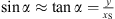 and
and  (see Fig. A1). The formula for the restoring force FS is then simplified to:
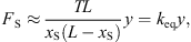 where keq = TL[xS(L − xS)]−1 is the equivalent stiffness of the hair for an in-plane vertical displacement y.
Let us suppose that the bow can rotate around an axis perpendicular to the x-y plane, passing through xS = 0. Let us assume that the only forces that act on the system are the restoring force  and the weight
 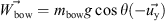 , where g is the gravitational acceleration. Using small-angle approximations, we obtain
 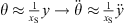 and cosθ ≈ 1. Applying the rotational form of Newton’s second law with these approximations leads us to the following equation of motion:
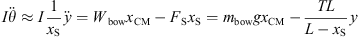
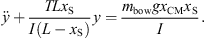
This equation describes the motion of a forced harmonic oscillator with a constant forcing term, due to the weight of the bow (right side of the equation). The oscillator is characterised by its natural angular frequency ω0, which depends on the tension of the hair T, the position of the loading point along the x-axis xS, and the rotational inertia of the bow I:
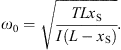
The constant force shifts the equilibrium position of the oscillator but does not affect its natural angular frequency ω0. Finally, the formula for the bouncing frequency of the bow in contact with the string is deduced from ω0 straightforwardly:
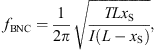 which is the same formula presented in [15].
Appendix B.
Signal detection theory concepts
Signal detection theory (SDT) begins with the premise that almost all reasoning and decision-making occur amidst some level of uncertainty. Below are all the concepts and formulas used in this paper.
B.1 Decision strategies
Three major decision strategies are commonly reported in the literature for A Not-AR and Duo-Trio tests: the likelihood ratio (β-strategy), the difference (τ-strategy), and the comparison-of-differences (COD-strategy, only for Duo-Trio) [35]. The β-strategy involves setting a criterion at some level of the ratio of the likelihoods of the two stimuli presented and then making a decision based on where the perceived ratio from the stimuli of a trial falls relative to this criterion. Conversely, the τ-strategy involves making a decision based on the comparison of the differences from both stimuli with the reminder. Finally, the COD-strategy is similar to the τ-strategy, but in this case, the absolute difference from both stimuli is taken into account (the sign of the difference is ignored).
For a given perceptual difference, these decision strategies influence discrimination performance (in terms of proportion of correct answers), which needs to be accounted for. Therefore, different formulas have been derived for calculating sensitivity indexes depending on the strategy. As only the τ-strategy has been hypothesised in this paper, only the formulas corresponding to this strategy will be presented here.
B.2 Protocol used in Nantes: A Not-AR test
The responses of the participants to an A Not-AR test, explained in Section 4.2, can be represented in a contingency table like Table B1. The stimuli S1 and S2 represent the bow presented after the reference bow A, and R1 and R2 the two possible answers.
Stimulus-response table for an A Not-AR test.
Participants’ sensitivity can be estimated from the distance between Hit (H) and False Alarm (F) rates, namely the d′ (d-prime) statistic. For a thoughtful but friendly explanation of this measure, let us refer to the work of O’Mahony [36]. H and F are defined as follows:
B.2.1 Sensitivity
The formula for calculating d′ in the case of a τ-strategy is the following:
![Mathematical equation: $$ {d\prime}=\sqrt{2}\left[{\mathrm{\Phi }}^{-1}(H)-{\mathrm{\Phi }}^{-1}(F)\right], $$](/articles/aacus/full_html/2025/01/aacus240059/aacus240059-eq39.gif) (B1)where Φ−1(P) denotes the operator giving the inverse of the normal cumulative distribution
(B1)where Φ−1(P) denotes the operator giving the inverse of the normal cumulative distribution  for the probability P, namely z-score.
The variance of d′ can be approximated from the variance of z-scores (see Chapter 13 in Hautus et al. [37]). These values follow an approximately normal distribution, with the following variance:
![Mathematical equation: $$ {\sigma }^2\left({\mathrm{\Phi }}^{-1}(P)\right)=\frac{P(1-P)}{N{\left[\phi \left({\mathrm{\Phi }}^{-1}(P)\right)\right]}^2}, $$](/articles/aacus/full_html/2025/01/aacus240059/aacus240059-eq41.gif) (B2)where ϕ(z) denotes the standard normal density function for the z-score and N the number of trials. The variance of d′ is then:
(B2)where ϕ(z) denotes the standard normal density function for the z-score and N the number of trials. The variance of d′ is then:
![Mathematical equation: $$ {\sigma }^2\left({d\prime}\right)=\frac{2H(1-H)}{{N}_1{\left[\phi \left({\mathrm{\Phi }}^{-1}(H)\right)\right]}^2}+\frac{2F(1-F)}{{N}_2{\left[\phi \left({\mathrm{\Phi }}^{-1}(F)\right)\right]}^2}, $$](/articles/aacus/full_html/2025/01/aacus240059/aacus240059-eq42.gif) (B3)where N1 and N2 are the number of trials of S1 and S2 respectively.
(B3)where N1 and N2 are the number of trials of S1 and S2 respectively.
B.2.2 Bias
SDT also gives a simple measure of bias, the criterion location c, calculated from H and F rates (see Chapter 2 in Macmillan and Creelman [23]):
![Mathematical equation: $$ c=-\frac{1}{2}\left[{\mathrm{\Phi }}^{-1}(H)+{\mathrm{\Phi }}^{-1}(F)\right] $$](/articles/aacus/full_html/2025/01/aacus240059/aacus240059-eq43.gif) (B4)
(B4)
![Mathematical equation: $$ {\sigma }^2(c)=\frac{1}{4}\left[{\sigma }^2\left({\mathrm{\Phi }}^{-1}(H)\right)+{\sigma }^2\left({\mathrm{\Phi }}^{-1}(F)\right)\right]. $$](/articles/aacus/full_html/2025/01/aacus240059/aacus240059-eq44.gif) (B5)
(B5)
When F exceeds the miss rate (1 − H), c turns negative, and vice versa. When those rates are similar, c tends to zero, indicating an absence of bias towards one response or the other. Extreme values of c, higher than 1 or lower than −1, occur when H or F are both large or small.
B.2.3 Confidence intervals and null hypothesis significance testing
To determine if d′ values are significantly greater than zero, a one-sided difference test is performed. The null hypothesis is H0 : d′ ≤ 0, i.e. there is no perceptual difference between both stimuli S1 and S2. The alternative hypothesis H1 : d′ > 0 posits that there exists a perceptual difference between them. For a confidence level α, the lower one-sided confidence bound is calculated as follows:
 (B6)where z1−α = Φ−1(1 − α) is the z-score for the confidence level 1 – α. The null hypothesis can be rejected at the α level if d′ = 0 falls below the lower bound of the interval, i.e. if
  . In this study, the typical value of α = 0.05 was consistently used.
The two-sided confidence interval would be used to test if d′ is greater than or less than a certain value. In our case, this approach does not seem appropriate to evaluate the difference with zero, since d′ should only grow in the positive way due to a greater difference between the stimuli. However, the two-sided confidence interval gives a general idea of the possible range of the true value of d′, reason why it is shown in Figures 9 and 12. It is also used to evaluate the significance of the difference between two d′ values, and it is calculated as follows:
![Mathematical equation: $$ \left[{d\prime}-{z}_{1-\alpha /2}\sqrt{{\sigma }^2({d\prime})},{d\prime}+{z}_{1-\alpha /2}\sqrt{{\sigma }^2({d\prime})}\right]. $$](/articles/aacus/full_html/2025/01/aacus240059/aacus240059-eq47.gif) (B7)
(B7)
Contrarily to d′, the criterion location c can take either positive or negative values depending on the bias. To determine if it is significantly different from zero, a two-sided test is performed with the null hypothesis H0 : c = 0 (no bias). The confidence interval of c for a confidence level α is:
![Mathematical equation: $$ \left[c-{z}_{1-\alpha /2}\sqrt{{\sigma }^2(c)},c+{z}_{1-\alpha /2}\sqrt{{\sigma }^2(c)}\right]. $$](/articles/aacus/full_html/2025/01/aacus240059/aacus240059-eq48.gif) (B8)
(B8)
The null hypothesis can be rejected at the α level if c = 0 falls outside the confidence interval.
B.3 Protocol used in Paris: Duo-Trio test
Before diving into the complexity of processing the sureness levels associated with the responses of the participants, let us first present the simple case, without taking them into account.
B.3.1 Duo-Trio test without sureness levels
For Duo-Trio tests, also called Two-Alternative Forced Choice with Reminder (2-AFCR) tests, a contingency table like that of the A Not-AR test (Tab. B1) is not possible, since both stimulus are presented in every trial. Participants were asked to choose which one, the first or the last, is equal to the reference stimulus. However, an analogous table (Tab. B2) can be constructed based on the order in which the stimuli are presented [23]. The stimuli S1 and S2 represent the two possible sequences, either with the reference in the first or last position, and R1 and R2 the two possible responses.
Stimulus-response table for a Duo-Trio test.
H and F rates are calculated from Table B2 similarly as for the A Not-AR test:
The sensitivity index for the τ-strategy can be calculated with the following formula [25]:
![Mathematical equation: $$ {d\prime}=\frac{1}{\sqrt{2}}\left[{\mathrm{\Phi }}^{-1}(H)-{\mathrm{\Phi }}^{-1}(F)\right]. $$](/articles/aacus/full_html/2025/01/aacus240059/aacus240059-eq50.gif) (B9)
(B9)
The calculation of the variance of d′ and the criterion location c, as well as their respective confidence intervals, is done similarly to the case of A Not-AR tests.
B.3.2 Duo-Trio test with sureness levels
When participants provide a sureness level for each answer, a table similar to Table B3 can be constructed. Each combination of sureness level and the accuracy of the answer (i.e., each column in Tab. B3) represents a distinct criterion for detecting a difference [38]. Using these criteria, a set of experimental points can be plotted in the FH-plane, forming the points of a receiver operating characteristic curve (ROC).
B3 Stimulus-response table for a Duo-Trio test with three sureness levels: NS (not sure at all/guessing), S (sure) and VS (very sure).
Experimental ROC points from Table B3 can be built using the next expressions:
 (B10)
(B10)
 (B11)
(B11)
Here, K is the total number of criteria (columns of Tab. B3) and 0 < k ≤ K. At first, the criterion for calculating H and F rate would be to consider the highest sureness, that is, the first column of Table B3. That gives the pair (H1, F1). Then the criterion would be lowered progressively to give the rest of the pairs.
The R-index is an estimator of the area-under-curve (AUC) of the aforementioned ROC curve. It quantifies the difference between two samples in terms of the probability of detecting such difference in a paired comparison. A R-index value close to 1.0 indicates that paired samples are easy to differentiate, while a value near 0.5 shows that those stimuli are not easily distinguishable. Supposing that both H and F follow normal distributions with equal variance, the R-index and its estimated variance  are related to the Mann-Whitney statistic U, defined as:
These relations were provided by Bi, equations (3) and (9) [38]:

![Mathematical equation: $$ {\widehat{\sigma }}^2(R)=\frac{1}{{N}_1{N}_2}\left[R\left(1-R\right)+\left({N}_2-1\right)\left({q}_1+{R}^2\right)+\left({N}_1-1\right)\left({q}_2-{R}^2\right)\right], $$](/articles/aacus/full_html/2025/01/aacus240059/aacus240059-eq56.gif) where q1 = q2 = F(x0),
where q1 = q2 = F(x0),  and F() represents the cumulative distribution function of a bivariate normal distribution with mean vector μ = (0, 0) and covariance matrix
  .
.
For 2-AFC tests (Two-Alternative Forced Choice tests), d′ and its estimated variance  can be linked to R as follows (Bi, Eqs. (29) and (30) [38]):
 (B12)
(B12)
 (B13)
(B13)
We assume that the previous equations are also applicable for Duo-Trio (2-AFCR) tests using a τ-strategy, since the value of d′ (Eq. (B9)) is the same as for 2-AFC tests [25].
From the value of d′ and its variance, the LCB and confidence interval used for hypothesis testing is calculated similarly than for the A Not-AR test (Eqs. (B6) and (B7)).
Appendix C.
ROC curves from Paris discrimination tests
The data points derived from the Paris discrimination tests using equations (B10) and (B11) are illustrated in Figure C1. In each case, a total of 18 points are computed, corresponding to 9 sureness levels for each of the 2 possible answers. The diameter of each marker is proportional to the number of points that share the same coordinates (ties). From the calculated values of d′ using equation (B12), a theoretical ROC curve is represented as a blue line, following the function F ↦ H derived from equation (B9):
 where Φ(z) is the operator giving the normal N(0, 1) cumulative distribution for the z-value. Consequently, the blue line depicted in each subfigure is not intended as a fit to the experimental points in the FH-plane, but rather represents the theoretical curve derived from the calculated value of d′ based on these points, under the assumption that all previously discussed conditions (including the use of a τ-strategy by all participants) are satisfied. The two-sided 95% confidence interval for d′ (Eq. (B7)) is represented as a filling around each ROC curve.
 |
Figure C1 Experimental ROC points and theoretical ROC curves (in blue) for the Paris discrimination tests. Holding test on the left, playing test on the right. From top to bottom: bows B, C, D and E. The 95% confidence interval for the theoretical curve is represented as a blue filling. |
References
- L. Cremer: The physics of the violin, MIT Press, Cambridge, MA USA, 1984. [Google Scholar]
- G. Bissinger: Bounce tests, modal analysis, and the playing qualities of the violin bow, Journal of the Catgut Acoustical Society 2, 8 (1995) 17–22. [Google Scholar]
- R. Caussé, J. Maigret, C. Dichtel, J. Bensoam: Study of violin bow quality, in: International Symposium on Musical Acoustics, Perugia, Italy, 10–14 September, 2001, pp. 1–6. [Google Scholar]
- F. Ablitzer: Influence des paramètres mécaniques et géométriques sur le comportement statique de l’archet de violon en situation de jeu, PhD Thesis, Université du Maine, Le Mans, 2011. [Google Scholar]
- F. Ablitzer, J.-P. Dalmont, N. Dauchez: Static model of a violin bow: Influence of camber and hair tension on mechanical behavior, Journal of the Acoustical Society of America 131, 1 (2012) 773–782. [CrossRef] [PubMed] [Google Scholar]
- J. Regh: Violin bow playability – A player’s view, 1st edn., Regh Publishing, Wappingers Falls, New York, USA, 2018. [Google Scholar]
- A. Tomezzoli, B. Michaud, E. Gagné, M. Begon, S. Duprey: Effect of bow camber and mass distribution on violinists’ preferences and performance, Frontiers in Psychology 12 (2021) 769831. [CrossRef] [PubMed] [Google Scholar]
- J. Stagg: Bow making and repair, John W Stagg Limited, 2016. [Google Scholar]
- C. Fritz, R. Viala, V. Salvador-Castrillo: Violinist, violin, bow: What can we hear and recognize? in: 24th International Congress on Acoustics, ICA2022, Gyeongju, Korea, 24–28 October, 2022. [Google Scholar]
- L. Capet: La technique supérieure de l’archet, Ed. Maurice Sénart et Cie., Paris, France, 1916. [Google Scholar]
- I. Galamian: Principles of violin playing and teaching, Prentice Hall, Englewood Cliffs, NJ USA, 1962. [Google Scholar]
- S.B. Shipps: The influence of Lucien Capet on teaching violin, American String Teacher 43, 1 (1993) 65–68. [CrossRef] [Google Scholar]
- S.A. Shock: Violin pedagogy through time: The treatises of Leopold Mozart, Carl Flesch, and Ivan Galamian, PhD Thesis, James Madison University, Harrisonburg, VA, USA, 2014. [Google Scholar]
- F.J. Testa: The science of the art of bowing, Violin Society of America 28th Conference 18 (2000) 173. [Google Scholar]
- A. Askenfelt, K. Guettler: The bouncing bow: Some important parameters, TMH-QPSR 38, 2–3 (1997) 53–57. [Google Scholar]
- D.A. Winter: Biomechanics and motor control of human movement, John Wiley & Sons, Hoboken, NJ USA, 2009. [CrossRef] [Google Scholar]
- E. Schoonderwaldt: Mechanics and acoustics of violin bowing, PhD Thesis, KTH Royal Institute of Technology, Stockholm, Sweden, 2009. [Google Scholar]
- K. Guettler: On the creation of the Helmholtz motion in bowed strings, Acta Acustica united with Acustica 88, 6 (2002) 970–985. [Google Scholar]
- A. Askenfelt: Measurement of bow motion and bow force in violin playing, The Journal of the Acoustical Society of America 80, 4 (1986) 1007–1015. [CrossRef] [Google Scholar]
- A. Askenfelt, K. Guettler: On the kinematics of spiccato and ricochet bowing, Journal of the Catgut Acoustical Society 3, 6 (1997) 9–15. [Google Scholar]
- C.E. Gough: Violin bow vibrations, Journal of the Acoustical Society of America 131, 5 (2012) 4152–4163. [CrossRef] [PubMed] [Google Scholar]
- V. Salvador-Castrillo, A. Picard, D. Spalletta, F. Ablitzer, C. Fritz: Towards understanding the influence of mass distribution on the perceived weight and force controllability of a violin bow, in: Forum Acusticum, Turin, Italy, 11–15 September, 2023, p. 877. Available at https://hal.science/hal-04292419v1. [Google Scholar]
- N.A. Macmillan, C.D. Creelman: Detection Theory: A user’s guide, 2nd edn., Lawrence Erlbaum Associates, Inc., Mahwah, NJ, USA, 2004. [CrossRef] [Google Scholar]
- S. Lau, M. O’Mahony, B. Rousseau: Are three-sample tasks less sensitive than two-sample tasks? Memory effects in the testing of taste discrimination, Perception & Psychophysics 66 (2004) 464–474. [CrossRef] [PubMed] [Google Scholar]
- M.J. Hautus, D. Van Hout, H.-S. Lee: Variants of A Not-A and 2-AFC tests: Signal detection theory models, Food Quality and Preference 20, 3 (2009) 222–229. [CrossRef] [Google Scholar]
- Y.-N. Jeong, B.-A. Kang, M.-J. Jeong, M.-J. Song, M.J. Hautus, H.-S. Lee: Sensory discrimination by consumers of multiple stimuli from a reference: Stimulus configuration in A-Not AR and constant-ref. duo-trio superior to triangle and unspecified tetrad? Food Quality and Preference 47 (2016) 10–22. [CrossRef] [Google Scholar]
- H.-K. Shin, M.J. Hautus, H.-S. Lee: Unspecified Duo-Trio tests can be as powerful as the specified 2-AFC: Effects of instructions and familiarization procedures on cognitive decision strategies, Food Research International 79 (2016) 114–125. [CrossRef] [Google Scholar]
- D. de la Prida, A. Pedrero, L.A. Azpicueta-Ruiz, M.Á. Navacerrada: Listening tests in room acoustics: Comparison of overall difference protocols regarding operational power, Applied Acoustics 182 (2021) 108186. [CrossRef] [Google Scholar]
- B. Rousseau, S. Stroh, M. O’Mahony: Investigating more powerful discrimination tests with consumers: Effects of memory and response bias, Food Quality and Preference 13, 1 (2002) 39–45. [CrossRef] [Google Scholar]
- M.-A. Kim, H.-S. Lee: Investigation of operationally more powerful Duo-Trio test protocols: Effects of different reference schemes, Food Quality and Preference 25, 2 (2012) 183–191. [CrossRef] [Google Scholar]
- J. Bi, M. O’Mahony, H.-S. Lee: The performance of the dual reference Duo-Trio (DRDT) method using a balanced-reference mode, Food Quality and Preference 48 (2016) 303–313. [CrossRef] [Google Scholar]
- Y.-J. Choi, J.-Y. Kim, R.H.B. Christensen, D. van Hout, H.-S. Lee: Superior performance of constant-saltier-reference DTF and DTFM to same-different tests by consumers for discriminating products varying sodium contents, Food Quality and Preference 37 (2014) 100–108. [CrossRef] [Google Scholar]
- C. Saitis, C. Fritz, G.P. Scavone, C. Guastavino, D. Dubois: Perceptual evaluation of violins: A psycholinguistic analysis of preference verbal descriptions by experienced musicians, Journal of the Acoustical Society of America 141, 4 (2017) 2746–2757. [CrossRef] [PubMed] [Google Scholar]
- V. Salvador-Castrillo, C. Fritz, G. Stoppani: Liens entre paramètres de facture, propriétés acoustiques et qualités perceptives sur un lot de 13 violons, in: 16ème Congrès Français d’Acoustique, CFA2022, Marseille, France, 11–15 April, Société Française d’Acoustique and Laboratoire de Mécanique et d’Acoustique, 2022. [Google Scholar]
- M. Hautus, D. Shepherd, M. Peng: Decision strategies for the two-alternative forced choice reminder paradigm, Attention, Perception & Psychophysics 73 (2011) 729–737. [CrossRef] [PubMed] [Google Scholar]
- M. O’Mahony: Understanding discrimination tests: A user-friendly treatment of response bias, rating and ranking R-index tests and their relationship to signal detection, Journal of Sensory Studies 7, 1 (1992) 1–47. [CrossRef] [Google Scholar]
- M.J. Hautus, N.A. Macmillan, C.D. Creelman: Detection Theory: A user’s guide, 3rd edn., Routledge, New York, NY, USA, 2021. [CrossRef] [Google Scholar]
- J. Bi: Statistical analyses for R-index, Journal of sensory studies 21, 6 (2006) 584–600. [CrossRef] [Google Scholar]
Cite this article as: Salvador-Castrillo V. Picard A. Spalletta D. Ablitzer F. & Fritz C. 2025. An experimental study on the perception of violin bow mass distribution. Acta Acustica, 9, 4. https://doi.org/10.1051/aacus/2024067.
All Tables
Bow mass configurations and corresponding mechanical properties. Δmt, Δmc, Δmf: added masses at the tip (64.5 cm from the pivot point), clamp (15 cm) and frog (−8.6 cm). mbow: total bow mass; xCM: distance from the centre of mass to the pivot point (represented in Fig. 3); I: moment of inertia with respect to the pivot point; ΔxCM, ΔI: variation of mechanical properties compared to the reference bow A, expressed as percentages. The mechanical properties of the bow without masses are as follow: mbow = 52.2 g, I = 4.75 gm2, xCM = 20.4 cm.
Results of the A Not-AR discrimination test. N is number of trials, nC is number of correct responses (“A” for the A-A pair, and “Not-A” for the other pairs). d′, c and their 95% confidence intervals (lower one-sided confidence bound, LCB, for d′ and two-sided confidence interval, CI, for c) are calculated with equations (B1), (B4), (B6) and (B8), presented in Appendix B. The variance for the confidence intervals has been calculated using equation (B3) for d′ and equation (B5) for c. The values of c whose CI exclude zero, and thus revealing a significant bias, are indicated in bold.
Sensitivity measure (d′) and bias measure (c) calculated from the results of the discrimination tests by holding and playing, presented in Figure 12. d′, c and their 95% confidence intervals (lower one-sided confidence bound, LCB, for d′ and two-sided confidence interval, CI, for c) are calculated with equations (B4), (B6), (B8) and (B12), presented in Appendix B. The variance for the confidence intervals has been calculated using equation (B13) for d′ and equation (B5) for c. The values of d′ whose LCB is higher than zero, and thus revealing a significant discrimination, are indicated in bold.
Classification of comments verbalised by the violinists in the free evaluation test. Representative comments in French for each sub-category are provided in quotation marks (translations to English by the authors).
Classification of comments of the category “Heaviness” stating changes in the perceived heaviness. The first three columns refer to evaluations at three specific bow parts: frog, middle and tip. Comments on changes of heaviness in general, without specifying exactly where, are counted in the fourth column.
B3 Stimulus-response table for a Duo-Trio test with three sureness levels: NS (not sure at all/guessing), S (sure) and VS (very sure).
All Figures
|
Figure 1 Overview of the violin bow main parts, without hair. |
| In the text | |
|
Figure 2 Detail of the role of the fingers. Left: the thumb and middle finger grip, creating a pivot point; top right: the little finger lifts the bow from the string; bottom right: the index finger presses the bow onto the string. Redrawn from Principles of violin playing and teaching (1st edn., p. 46 and 49) by I. Galamian, 1962, Prentice Hall [11]. |
| In the text | |
|
Figure 3 Vertical forces acting on the bow in three different scenarios where the bow remains horizontal. (a) Holding the bow horizontally in the air. (b) Bowing the string close to the frog (0 ≤ xS < xeq). (c) Bowing the string close to the tip (xeq ≤ xS < L). |
| In the text | |
|
Figure 4 Resulting force on the string during a stroke with two different finger-bow interactions. The mechanical properties of the bow and the distances of the fingers to the pivot point are assumed to be as follows: mbow = 60 g, xCM = 20 cm, xI = 6.3 cm, xL = 5.6 cm. (a) Resulting force on the string when the index and little finger forces are null. (b) Finger forces required to obtain a uniform force on the string of 1 N, as presented in equation (3). |
| In the text | |
|
Figure 5 Vertical forces and motion of the bow in two different cases where the bow is rotated around the pivot point. (a) Shaking the bow up and down in the air. (b) Bouncing “naturally”, i.e. without any interaction of the fingers except keeping the pivot point fixed (little and index finger forces equal to zero). |
| In the text | |
|
Figure 6 Experimental bow with added masses. Top: close-up of the magnets (bow B of Tab. 1). Bottom: participants’ view of the bow, with the tip and frog magnets covered with paper and a lightweight piece of foam covering the magnetic clamp. |
| In the text | |
 |
Figure 7 Mechanical properties of the bows presented in Table 1. |
| In the text | |
|
Figure 8 Set-up for the measurement of the bow oscillations and recorded motion of the bow’s tip. The bow-plus-peg was suspended from a thin cylindrical metallic rod. |
| In the text | |
|
Figure 9 Sensitivity d′ values from Table 2, with two-sided 95% confidence intervals (Eq. (B7) in Appendix B). The variance for the confidence intervals has been calculated using equation (B3). |
| In the text | |
|
Figure 10 Distribution of responses for both holding and playing discrimination tests (Duo-Trio). The horizontal axis represents the two qualities of the responses: correctness, with incorrect responses shown in red on the left and correct responses in green on the right; and sureness, which ranges from 1 (not sure at all, guessing) to 5 (absolutely sure) in 0.5-point intervals. The marker type represents the real position of the reference bow A: circles when it was presented in first (holding test) or second (playing test) position, and crosses when it was presented last. There are N = 20 responses for each test and bow pair, corresponding to 20 participants. The distribution of responses for all bows, that is, the combination of all responses from each test regardless of the bow, is represented as a blue filling. |
| In the text | |
|
Figure 11 Average sureness level without considering correctness (i.e. overall sureness), represented with blue vertical lines: 2.56 for the holding test and 2.91 for the playing test. The color and marker type for the responses follow the same convention as in Figure 10. |
| In the text | |
|
Figure 12 Sensitivity d′ values from Table 3, with two-sided 95% confidence intervals (Eq. (B7) in Appendix B). The variance for the confidence intervals has been calculated using equation (B13). |
| In the text | |
|
Figure 13 Percentages of the four main perceptual categories resulting from the semantics collected during the free evaluation test. S: Spiccato; H: Heaviness; P: Playability; O: Other (sound quality, preference, etc.). Total number of comments: 49 for test A → C and 47 for test A → E. |
| In the text | |
|
Figure 14 Finger forces necessary to exert a constant force on the string FS, for all the possible distances between the frog of the bow and the hair-string contact point xS. Two bows are represented, A and E, and two constant vertical forces on the string FS = 1 N and FS = 0.1 N. |
| In the text | |
|
Figure A1 Forces on the bow (top) and on the loaded hair (bottom). The vertical axis of the loaded hair has been amplified to aid in visualizing the forces. |
| In the text | |
|
Figure C1 Experimental ROC points and theoretical ROC curves (in blue) for the Paris discrimination tests. Holding test on the left, playing test on the right. From top to bottom: bows B, C, D and E. The 95% confidence interval for the theoretical curve is represented as a blue filling. |
| In the text | |
Current usage metrics show cumulative count of Article Views (full-text article views including HTML views, PDF and ePub downloads, according to the available data) and Abstracts Views on Vision4Press platform.
Data correspond to usage on the plateform after 2015. The current usage metrics is available 48-96 hours after online publication and is updated daily on week days.
Initial download of the metrics may take a while.