| Issue |
Acta Acust.
Volume 9, 2025
|
|
|---|---|---|
| Article Number | 63 | |
| Number of page(s) | 13 | |
| Section | Musical Acoustics | |
| DOI | https://doi.org/10.1051/aacus/2025038 | |
| Published online | 22 October 2025 | |
Cartography of a trombone sound regimes using a python implementation of a Support Vector Machine-based Explicit Design Space Decomposition
1
Laboratoire Manceau de Mathématiques, Le Mans, France
2
Laboratoire d’Acoustique de l’Université du Mans (LAUM), UMR CNRS 6613, Institut d’Acoustique – Graduate School (IA-GS), CNRS, Le Mans Université, France
* Corresponding author: This email address is being protected from spambots. You need JavaScript enabled to view it.
Received:
1
April
2025
Accepted:
25
July
2025
Abstract
Self-sustained musical instruments are non-linear dynamical systems that can produce a large number of sound regimes, whose existence and stability depend on both design and a number of control parameters. Determining which regimes exist for given parameters and which one is reached in practice when several stable regimes coexist for identical parameters is of importance from both the making and playing points of view. In this article, we consider a physical model of a trombone, and produce cartographies of the sound regimes in the space of playing parameters associated to the musician, namely the blowing pressure and the lips parameters. In practice, boundaries of the parameters space regions corresponding to different regimes are defined explicitly using Support Vector Machines. This approach is implemented in an open-source python library pyEDSD which is presented here. Importantly, the method is not specific to the considered application and the library may be of interest for other applications, in particular in engineering.
Key words: Brass instrument / Machine learning
© The Author(s), Published by EDP Sciences, 2025
 This is an Open Access article distributed under the terms of the Creative Commons Attribution License (https://creativecommons.org/licenses/by/4.0), which permits unrestricted use, distribution, and reproduction in any medium, provided the original work is properly cited.
1 Introduction
As non-linear dynamical systems, musical instruments produce a diversity of oscillation regimes, whose existence and stability depend, often sensitively, on a large number of parameters [1–3]. Here we focus on brass musical instruments, which include, among others, the trumpet and the trombone. In these instruments, the main control parameters are the blowing pressure, the lips mechanical properties (often referred to as “embouchure parameters”) and the configuration of the instrument acoustical resonator, which the musician can change by moving the slide (for the trombone) or by changing the fingering (for the trumpet) [4]. Importantly, for a given configuration of the resonator, several periodic sound regimes (musical notes) with different fundamental frequencies are produced depending on the playing parameters chosen by the musician such as the blowing pressure and the lips natural frequency [5, 6]. Characterising the dependency of the obtained sound regimes on the playing parameters is of practical importance both from a making and playing point of view.
The study of the different regimes of brass instruments is the subject of a large body of the literature [4–8] and is complicated by the fact that the model is non linear, and that the control parameters are not well known [9]. The present study aims at simplifying the set up of such studies which are often quite slow when the model behaviour is investigated systematically under the slow variation of a parameter (e.g. poor man’s continuation) or more difficult to implement (continuation [10]).
A possible way to investigate the regimes of a non-linear dynamical system in general and in a model of wind musical instrument in particular is to discretise the parameters space and simulate the model for each point (i.e. each set of parameters), to determine which regime is reached after any transient dynamics has died out. This strategy has been used in [1] but quickly becomes time-consuming when the discretisation gets finer due to the large number of simulations to perform. A more refined method, based on the Explicit Design Space Decomposition (EDSD) technique developed in the series of papers [11–16], has been proposed in [17] and used in [18, 19] to study the clarinet regimes. The EDSD method computes a decomposition of the so-called design space (here the space of control parameters) using Support Vector Machines (SVM) which are easily computable functions whose set of zeros defines the boundary of regions in which the different regimes are observed. Compared to the discretisation of the parameters space, this approach requires a much lower number of time-domain simulations of the considered model.
Here we introduce the python library pyEDSD, which computes a SVM decomposition of the design space with respect to a black box function. It is largely inspired by the aforementioned works on EDSD which led to the part of the CODES Matlab library dedicated to EDSD1. The possibilities of pyEDSD are illustrated here on a physical model of a trombone: in the space of the blowing pressure and lip resonance frequency (the two main control parameters) we compute the boundaries between the different observed periodic regimes for a given set of initial conditions. The library itself is introduced in Section 2: notions on main elements of the method, such as SVM, are recalled and the possibilities of pyEDSD are illustrated in explicit examples coded in python. In Section 3, the method is applied to the cartography of the different periodic regimes (corresponding to musical notes) of the trombone in the space of the two main control parameters of the musician. This section also entails a discussion on the so-called complex and real representations of the input impedance, and gives further reasons for favouring the real one.
2 Explicit design space decomposition based on Support Vector Machine
Support Vector Machines (SVM) are a class of machine learning technique which has been widely used for classification tasks. The underlying idea is to generate an explicit (linear or non-linear) decision function that corresponds to the boundary between different classes in a space of relevant parameters. SVM have originally been developed in the linear case by Vapnik in [20] and have since been expanded and used in many different areas. It was notably generalised in [21] for non linear kernels. The interested reader can refer to dedicated textbooks such as [22, 23] as entry points to the literature. In the following, we detail only the few properties that are necessary for the EDSD implementation (cf. Sect. 2.4).
In pyEDSD, the SVMs are computed using the library scikit-learn, [24].
2.1 Definition of Support Vector Machines
We first present here the binary SVM which aims to classify points associated to labels a or b, for two distinct classes a and b.
Let x1, …, xN ∈ ℝd be points and y1, ⋯, yN ∈ {a, b} their labels. A decision function is a map D: ℝd → ℝ such that for all i, D(xi)> 0 if yi = a and D(xi)< 0 if yi = b.
The Support Vector Machine algorithm is a classifier that produces a decision function verifying the maximum-margin property. In the practical case considered here, the zeros of the decision function correspond to the boundary between regions of the plane of two parameters associated to different sound regimes. The maximum-margin property requires that the distance from the separating subset D−1({0}) to the set of points xi is maximal, as illustrated in Figure 1. In the linear case, this notion is relatively self explanatory as the distance from a set of points to a hyperplane is easy to compute. In the non-linear case, this is not as easy, and is achieved by using the kernel trick, which uses an embedding in a larger dimensional space [21].
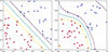 |
Figure 1 Theoretical example of a SVM in the square [0, 1]2 obtained with scikit-learn. The left panel is linear, the right panel is radial. The labels are represented by different colours, red and blue. The cyan curve represents the separation between regions associated to different labels. The yellow and purple curves represent the limits of the specified margins around the boundary. |
One of the maximum-margin property advantages is that it makes the decision function unique (when it exists), and ensures the best possible separation.
The library scikit-learn, through the function svc, handles different types of kernels. The following ones are directly implemented, but the user can also specify their own:
-
Polynomial K(x, y)=(⟨x, y⟩+r)d;
-
Gaussian radial K(x, y)=e γ∥x − y∥2 for γ > 0;
-
Sigmoid function K(x, y)=tanh(κ⟨x, y⟩+c) with κ > 0 and c < 0.
The decision function is then of the form
 (1)
(1)
where the α k are parameters calculated using the SVM algorithm through an optimisation procedure (cf. loc. cit. for more details).
As the SVM uses Euclidean distance, the result may not be satisfactory if the variations of different coordinates of the data do not have the same magnitude. As is usually the case when comparing data with different units, pyEDSD performs all its SVM computations with dimensionless data.
2.2 Multi-class SVM
Many strategies have been proposed to generalise SVMs to multi-class classification [22, 23]. The one used in pyEDSD is the so-called “One versus One” (abbreviated as “ovo”) because it lends itself well to the generation of points on the boundary (cf. Sect. 2.3).
Being given labelled points (x
i
, y
i
)∈ℝ
d
× L, with L a set of ℓ ordered labels, the strategy “ovo” defines  binary classification problems, one for each ordered pair ν = (a, b) with a, b ∈ L, a < b. The SVM algorithm can then produce decision functions D
(a, b), such that
binary classification problems, one for each ordered pair ν = (a, b) with a, b ∈ L, a < b. The SVM algorithm can then produce decision functions D
(a, b), such that
A linear multi-class SVM is shown in Figure 2. We can see on this example that, for the purpose of classification, the boundary between classes 0 and 2 is actually useless. This property is used for the multi-class EDSD detailed in Section 2.5.
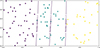 |
Figure 2 Example of a multi-class SVM. A posteriori, the boundary in the middle could have been discarded, see Section 2.5. |
2.3 Finding points on the boundary of the SVM
Let D: C → ℝ be a decision function (or actually any sufficiently regular function) defined over a rectangular cuboid C. The goal of this section is to produce points on the boundary ∂D = D −1(0) between the positive and negative regions defined by D.
The first step is to take a random point x 0 in the search domain C which serves as a starting point to a minimization procedure of the function x ↦ D(x)2. The algorithm chosen for pyEDSD is the gradient algorithm, which has the advantage of being simple and effective. The idea is that if x 0 is close enough to the boundary of D then the convergence should be the fastest, provided D is sufficiently smooth, which is necessarily the case thanks to the choice of a regular kernel for the SVM.
Note that in the original article [16], it is moreover enforced that the points generated on ∂D are the furthest away from each other.
An example is given in Figure 3, for a decision function classifying the inner and outer points of a trifolium (obtained using pyEDSD), and the search space C = [ − 2, 2]×[−2, 2].
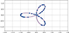 |
Figure 3 Example of random points created on the boundary of an SVM. For this example, all points verify |D(x i )| < 7.10−8. |
Because the points of the boundary are independent from one another, the generation can be parallelized by choosing different stating points x 0 for each thread.
2.4 The full algorithm
The full algorithm is now detailed for a given black-box function β: C → {a, b} that classifies each point in the parameter space in a class.
First let X ⊂ C be a finite set, which should contain at least one element in each class and let N 0 be an integer. The algorithm first step is the production of a set of N 0 points in C using a pseudo-random generator, to add them to X and to evaluate the black-box function β on all points of X to produce the list of labels Y. A first decision function D 0 is then computed using the scikit-learn library.
An iterative process subsequently starts, with w parallel threads. First, w random points are computed on the boundary ∂Dn of the classifier, and the classifier criterion β is evaluated on these new points, which are then added to X and their label to Y. A new classifier Dn + 1 is then computed and a new step of the loop is performed. The pseudo-code for the algorithm is given in Algorithm 1, where the parallelizable parts are shown in blue.
Input : β C, X, N0, N1, w
X0 ← N0 pseudo-random points in C
X ← X ∪ X0
D ← SVM(X,Y)
while N1 ≠ 0 do
X, Y ← X ∪ X′, Y ∪ Y′
D ← SVM(X, Y)
N1 ← N1 – w
Output : D
2.5 Generalisation to multi-class classifiers
2.5.1 With the “ovo” strategy
The algorithm detailed in the previous section can be adapted to multi-class black box functions using the “ovo” strategy (cf. Sect. 2.2) and the pairwise decision functions D (a, b) for every ordered pair of classes with a < b.
Regarding the impact on Algorithm 1, it means that the generation of additional points must be done on the frontiers of every decision function D
(a, b), which contains  elements, where ℓ is the number of classes. However, this can be reduced as there may be regions which are not neighbours, such as the boundary between classes 0 and 2 in the example in Figure 2. Some decision functions can therefore be discarded and the search can be performed over a subset specified by the user and denoted neighbours in pyEDSD, which contains a list of the pairs (a, b) relevant for the computation; see the trombone regime example in Section 3.
Once the final decision functions are obtained, it is possible to define a decision function for one class: first, if a > b, define D (a, b) = −D (b, a), then define
![Mathematical equation: $$ \begin{aligned} D_a(x) = \max _{\begin{matrix} b \in [\![0, n ]\!]\\ b \not = a \end{matrix}}D_{(a, b)}(x). \end{aligned} $$](/articles/aacus/full_html/2025/01/aacus250034/aacus250034-eq5.gif) (2)
(2)
If β(x)=a, then D
(a, b)(x)< 0 for all  and D
a
(x)< 0. The function D
a
can then be studied on its own, be it for displaying or measuring purposes (see Sect. 2.6).
and D
a
(x)< 0. The function D
a
can then be studied on its own, be it for displaying or measuring purposes (see Sect. 2.6).
Note that, due to the use of the max in formula (2), D a may not be as regular as the decision functions. Therefore the gradient algorithm used to produce points on the boundary may not be able to converge in the neighbourhood of “corners”.
The generation of random points in the refinement step are produced for one particular decision function, each of them therefore gets as an average of N 1/#neighbours points in its boundary. To get a good result, the number of neighbours must then be as small as possible, or N 1 must be increased. The example file multiclass_2d.py of the library gives a full example and is reproduced below.
2.5.2 With the “ovr” strategy
The “ovo” strategy of pyEDSD can be useful for a preliminary exploration of the parameter space, when classes are not all well identified. However, it can be quite slow due to the refinement points distribution among all the neighbours. Depending on the problem, it may be faster to use binary classifiers once classes are identified. This can be readily obtained with a loop for all the classes a using the “ovr” strategy that uses the binary classifier returning true if the output of β is a. An example is shown in the example below, in which only the “main” part of listing Algorithm 2 is changed to give Algotihm 3.
import pyEDSD as edsd
def func(X) :
r =(X[0]**2+X[1]**2)**0.5
if X[1] < 0 : return(0)
return(1+min(3, int(2*r)))
if _ _name_ _ = = "_ _main_ _" :
bounds = [[-2, -2], [2, 2]]
X0 = [[0, 0], [0.5, 0.5], [1, 1],
[1.5, 1.5]]
clf = edsd.edsd(func, X0=X0, bounds=bounds,
processes=4, N0 = 20, N1 = 1000,
svc=dict(C = 100),
neighbours = [[1,2], [2, 3],
[3, 4], [0, 1], [0, 2], [0, 3], [0, 4]])
edsd.save(clf, "multi.edsd")
for c in Classes :
def f(X) :
return(func(X) == c)
clf = edsd.edsd(func, X0=X0, bounds=bounds,
processes=4, N0 = 20, N1 = 1000,
svc=dict(C = 100))
edsd.save(clf, f"multi-{c}.edsd")
2.6 Computation of regions descriptors using Monte-Carlo methods
For a given decision function D, either that of a pair D (a, b) given directly as an SVM, or one D a coming from a multi-class SVM as in Section 2.5 equation (2), it is possible to use the generation of points on the boundary ∂D and Monte-Carlo methods to evaluate some quantities like
-
max and min of coordinates of points (to obtain a bounding box),
-
distances to a point,
-
center of gravity,
-
radius of D.
As an example, the trifolium diameter evolution is shown in Figure 4 with respect to the number n of points on the boundary. In this figure, the computation time at each step is also shown with and without parallelisation (for 20 parallel threads).
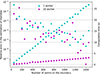 |
Figure 4 Evolution of the relative error in the estimation of the diameter (circles) of the trifolium as represented in Figure 3, and corresponding computation time (crosses) with the number of points on the boundary. Cyan and purple colors correspond to the case of one and 20 workers respectively. |
Note that, although the error in the diameter estimation tends to 0 with n, for a fixed n the error is of the form O(diameter/n) in the uniform case scenario.
With the same technique, it is also possible to obtain a mesh of the interior. For this pyEDSD first generates points on the frontier ∂D, from which it extracts a bounding box. Then it generates uniformly distributed random points in this box, of which only those that verify D < 0 are kept. The last step is to generate the Delaunay triangulation using the points on the boundary and the points in the inside. Note that the Delaunay triangulation is actually computed on the inhomogeneous data as it may otherwise give unbalanced meshes. Once a triangulation is computed, other quantities can be estimated, such as the volume inside ∂D. An example of such a triangulation is given in Figure 5.
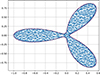 |
Figure 5 Example of a SVM constructed with Algorithm 1 and a mesh obtained with the method described in Section 2.6. The bounding box is also computed using the boundary points. |
3 Application to the trombone regimes
Velut et al. [5] computed, for a given lip frequency, the mouth pressure threshold at which the equilibrium (non oscillating) regime becomes unstable, often leading to the production of a periodic regime corresponding to a note. This provides insight on the ease of playing of the different regimes of a trombone. We aim here at reproducing and expanding these results by taking advantages of the pyEDSD library capabilities.
3.1 Physical model
An elementary trombone model is used here. It is detailed in [4], Chapter 5. It is the same as the one used in [5] and consists of a set of three equations describing
-
(1)
the lip opening h through a second-order differential equation that takes the form of a one degree of freedom oscillator,
-
(2)
the trombone input impedance describing the resonator response in the frequency domain,
-
(3)
the input air flow modulated by the lips vibration
see equation (6).
In this model, the lips motion depends on four parameters: the lip opening at rest H, their quality factor Q ℓ, surface density μ ℓ and resonance frequency F ℓ. The reference values for these lips parameters are taken from [5] and summarized in Table 1. Note that these values may not be realistic, in particular that of Qℓ, but are kept as such for comparison with the existing literature.
The second equation of the model comes from the input acoustical impedance of the resonator Z = P/U written in the Fourier domain, where P and U denote respectively the Fourier transform of the downward pressure p and that of the flow through the reed channel u. A modal decomposition of the impedance is then performed
 (3)
(3)
where ω is the pulsation, N is the number of modes considered in the approximation of the impedance, the bar ¯ denotes the complex conjugation,  denotes the characteristic impedance with ρ the air density, c the speed of sound in air, and S the trombone mouthpiece entry section. The modal parameters C
n
and s
n
are computed using the Rational Fraction Polynomial method [25] that approximates measurements of the input impedance of a Courtois trombone. With no extra condition, one obtains the so-called ℂ-representation. If the extra condition
denotes the characteristic impedance with ρ the air density, c the speed of sound in air, and S the trombone mouthpiece entry section. The modal parameters C
n
and s
n
are computed using the Rational Fraction Polynomial method [25] that approximates measurements of the input impedance of a Courtois trombone. With no extra condition, one obtains the so-called ℂ-representation. If the extra condition  is added (see Eq. (7.23) in [26]), ensuring that the impedance is zero at zero frequency, the decomposition uses a real mode basis and is called the ℝ-representation. A ℝ-representation can be obtained from the complex one using the technique described by Ablitzer [27].
The downstream pressure (i.e. the acoustic pressure in the mouthpiece) can then be written as
 (4)
(4)
with the complex components p n satisfying the differential equation
 (5)
(5)
coming from a frequency-domain formulation (3) obtained through an inverse Fourier transform, where u denotes the flow through the lips. This is equivalent to 2N real differential equations.
Finally, the flow u entering the instrument resonator and which is modulated by the lips opening h is described by a Bernoulli law in the third line of (6). Note that as h is allowed to be negative, the reed entering section in this equation is set as wmax(h, 0). Moreover, because of the possible inversion of the flow direction, the Bernoulli law must be regularized along the lines of [6] using a dimensionless parameter ε taken for the simulations to be 10−6.
The final set of equations is therefore
 (6)
(6)
where P c r = μ ℓ H ω ℓ 2 is a physical parameter homogeneous to a pressure, equivalent to the closing reed pressure for reed instruments.
The model defined by equation (6) gives a system of 2N + 2 coupled ordinary differential equations with the vector of state variables

depending on design parameters (which are fixed here and encoded in the input impedance) and control parameters  comprised of the downstream pressure p
m
and lips parameters H, F
ℓ, μ
ℓ and Q
ℓ. It can be solved for any given set of initial conditions using an ODE solver. For this study, we chose either a simple Runge–Kutta solver of order four, or an implicit trapezoidal rule solver for extra stability. Both are implemented in C for extra speed, with a sampling frequency f
s
= 48 000 Hz which is sufficient to ensure convergence.
comprised of the downstream pressure p
m
and lips parameters H, F
ℓ, μ
ℓ and Q
ℓ. It can be solved for any given set of initial conditions using an ODE solver. For this study, we chose either a simple Runge–Kutta solver of order four, or an implicit trapezoidal rule solver for extra stability. Both are implemented in C for extra speed, with a sampling frequency f
s
= 48 000 Hz which is sufficient to ensure convergence.
3.2 Definition and detection of the regimes
When that the impedance is zero at zero frequency, the model (6) has a static equilibrium solution

with
which exists for any values of p m and lip parameters, but whose stability depends on these parameters [5]. Physically, this solution corresponds to the fact that no sound is produced despite the fact that the musician blows into the instrument.
Let Ξ0 = (0, …, 0) be the null state vector , which is chosen as a fixed set of initial conditions, and  a set of control parameters (p
m
, H, F
ℓ, μ
ℓ, Q
ℓ). The first step is to compute which regime is reached by the system for these initial conditions and a given set of control parameters.
a set of control parameters (p
m
, H, F
ℓ, μ
ℓ, Q
ℓ). The first step is to compute which regime is reached by the system for these initial conditions and a given set of control parameters.
3.2.1 Obtaining the periodic regime
The final regime computation is obtained by simulating successively segments of length Θ and checking if the last one is periodic. If so, the iterative process is over and the regime can be identified. Otherwise, a new segment is computed using the ODE solver applied to system (6) using as initial conditions the last computed values of the previous segment.
The criterion chosen here to detect if the permanent regime is reached relies on the signal envelope. For this, the duration of the simulated time series must be much longer than any possible signal oscillation period, i.e. Θ ≫ 1/F 1 where F 1 denotes the smallest expected frequency for periodic regimes coming from Table 2.
Frequencies of the first seven input impedance peaks of a Courtois T149 trombone fitted with a bass trombone mouthpiece Holton 181. The first row indicates the peak number.
First, two “pathological” cases must be dealt with: that of an unbounded signal labelled "Nan" and which exists mainly when the numerical scheme does not converge, and that of a signal going toward zero, labelled "0", for which the envelope criterion cannot be used. Both are detected using bounds on the downstream pressure absolute value computed on a segment. For the first case, the maximum must be smaller than a given bound, and bigger than another bound in the second case.
With these two cases aside, the quantity
![Mathematical equation: $$ \begin{aligned} \tau (p_m) = -\frac{\log _{10}\left(\frac{\max \left\{ p_m(t), t \in \left[\mathrm{\Theta }-1/F_1, \mathrm{\Theta }\right]\right\} }{\max p_m}\right)}{\mathrm{\Theta }-1/F_1} \end{aligned} $$](/articles/aacus/full_html/2025/01/aacus250034/aacus250034-eq19.gif) (7)
(7)
approximates the signal envelope logarithmic slope. If it is smaller than a given bound, then the simulated signal is considered to be permanent. Otherwise a new segment is computed. Note that if the signal converges toward 0, this logarithmic slope may not be small.
This leads to another pathological case: depending on the control parameters  , the system can show slow convergence towards the periodic regime, which amounts to a small logarithmic slope, which remains larger than the fixed bound for a long time. It is therefore necessary to fix a maximal duration of the simulated time series. If the iterative process has not found a permanent regime after this number, the signal is labelled as "Slow".
3.2.2 Identification of the regime
We can now suppose that the envelope logarithmic slope is almost zero and that a permanent regime has been reached. The instantaneous frequency F of the downstream pressure computed during the last segment is obtained using the Yin algorithm [28] which comes with an indicator of periodicity: the harmonic ratio.
If the harmonic ratio is bigger than a given reference value h r ref = 10−3, then the steady-state solution is aperiodic and β(ℭ) ="Non periodic". This may encapsulates many different kind of regimes worth studying, but they are not the focus of the present study. When the harmonic ratio is smaller than the reference, the solution is considered to be periodic.
Figure 6 shows periodic signals obtained for the lip parameters of Table 1, a mouth pressure pm = 6000 Pa and different values of Fℓ. In this figure, the playing frequency is slightly above one of the acoustic resonancefrequency, given in Table 2. This is a general case for the kind of lip models considered here (cf. [4], Fig. 5.6b). Although different from the others, the waveform obtained for Fℓ = 52.98 Hz is reminiscent of those obtained by Elliott in [29].
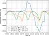 |
Figure 6 Periodic part of signal obtained from system (6) with ℝ-decomposition of the input impedance, mouth pressure pm = 6000 Pa, lip parameters from Table 1 and 3 different lip frequencies Fℓ. |
We therefore define the regime towards which the system converges as the nth register, where n corresponds to the highest resonance peak index with frequency smaller than the playing frequency
 (8)
(8)
On the other hand, if the logarithmic envelope is smaller than a reference τ(p)≥τ ref = 10−2, then the stable solution has not been reached during the mth simulation segment, so that we should iterate to the next m unless it is bigger than a reference m max, in which case the solution must be very close to a frontier between regimes, and β(ℭ) = "Slow".
This regime definition can be summarized with the pseudocode detailed in Algorithm 4.
Input : pm, ℭ = (Fl, μl, Ql, H)
m ← 0, Ξinit ← Ξ0
while m < mmax do
Ξ ← ODE solution with initial condition Ξinit
p ← pressure(Ξ)
if max(p) = Nan then return "Nan"
if max(p) < pref then return "Silent"
if τ(p) < τref then
F, hr ← Yin(p)
if hr < hrref then
return max{n, F ≥ 𝔍(sn)/(2π)}
else return "Non periodic"
Ξinit ← Ξ(Θ)
m ← m + 1
return "Slow"
Output : Regime
Figure 7 shows the different regimes obtained for the lip parameters given in Table 1 and computed for each lip frequency using Algorithm 4. The regime 0, where no sound is produced and the downstream pressure tends to 0, is represented by gray rectangles.
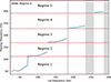 |
Figure 7 Evolution of the playing frequency with respect to lip frequency, obtained with Algorithm 4 for each lip frequency and initial condition Ξ0. The lip parameters are those of Table 1, the mouth pressure is pm = 6000 Pa and the program uses a ℝ-representation of the input impedance. |
3.3 Mouth pressure oscillation threshold
To assess the precision of pyEDSD, the oscillation thresholds – corresponding to the minimal value of the mouth pressure for which an oscillation is produced for the considered initial conditions – are computed here on a range of lip frequency values. The results are compared with those of [5, 6], obtained through a bifurcation analysis, as illustrated in Figure 8.
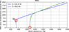 |
Figure 8 Map of regimes 1 to 6 obtained with pyEDSD, together with theoretical pressure threshold as a red dotted line obtained with auto-07p. |
For a given set of control parameters, the mouth pressure threshold can be computed using bifurcationdiagrams, such as that of Figure 9 which is obtained using the continuation software auto-07p [30].
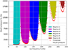 |
Figure 9 Bifurcation diagrams representing the evolution of root mean square value of the downstream pressure p with respect to the mouth pressure pm, for the lip parameters of Table 1 and two different values of the lip frequency: Fℓ = 101.8 Hz (blue curve) and Fℓ = 93.2 Hz (green curves). Stable and unstable parts of the branches are represented by solid and dashed lines, respectively. The pressure threshold is indicated in each case by a red circle. |
In this figure, two bifurcation diagrams are shown for lip parameters given in Table 1 and two different lip frequencies. For the smaller lip frequency (Fℓ = 93.2 Hz, green curve), the Hopf bifurcation is direct, and the pressure threshold corresponds to the destabilisation threshold of the equilibrium solution obtained by a linear stability analysis. However, for the larger lip frequency (Fℓ = 101.8 Hz, blue curve) the Hopf bifurcation is inverse, and the emerging periodic solution is unstable (dashed part of the curve) until a saddle node bifurcation of periodic orbits is reached, which gives the pressure threshold. Note that the combination of the inverse Hopf bifurcation and saddle node bifurcation of periodic orbits induces a difference between the destabilisation threshold of the equilibrium solution and the threshold defined as the minimal blowing pressure for which a sound can be produced. Here however this difference is small, as shown in [6].
3.4 Pressure threshold obtained with pyEDSD
Algorithm 4 is used as a black box parameter function β for pyEDSD, where only the mouth pressure pm and lip frequency Fℓ are used as free parameters and Table 1 is used to get a full set of lip parameters. For comparison purposes, β must return only one type of data, and in the example below all the regimes are strings.
To make sure points in each class are produced during the initialisation phase of pyEDSD, the variable X0 must contain points in each class. This is obtained by picking high mouth pressure values (18 kPa) for a discretized set of lip frequencies. That part of the initialisation process uses a priori estimates of the mouth pressure, and it can be found in [6]. According to the definition of regimes, the set of possible classes is composed of
-
1 silent regime, "Silent";
-
6 different periodic regimes, "1" to "6";
-
1 regime indicating numerical scheme instability, "Nan";
-
1 aperiodic regime, "Non periodic", which may contain many different regimes;
-
1 slow convergence regime, "Slow".
We thus have 10 different regimes, and therefore  possible neighbouring regimes. However, during the exploratory phase, it is better not to set the neighbours variable as it is not clear what class is close to another, so the set of neighbours in this example is the full set.
The main function of pyEDSD is launched by setting the number of parallel workers for the search of points on boundaries, the size N0 of pseudo-random discretisation of the search space, and the total number of points N1 on boundaries. The number of refinement steps (“while” loop in Algorithm 1) is therefore N1/#workers.
The full program (except the black box function β) is given in Algorithm 5. The full computation time is 120 s using 16 cores on a desktop computer.
bounds = [[0, 10], [350, 2e4]]
X0 = [[f, 18e3]
for f in np.linspace(100, 350, 50)]
clf = edsd.edsd(beta, X0=X0, bounds=bounds,
processes = 16, N0 = 200, N1 = 5000,
svc=dict(C = 1000))
Figure 8 shows the regions corresponding to the different classes in the (Fℓ, pm)-plane of control parameters, as obtained with the program above for the 6 periodic regimes, together with the pressure threshold at which the static regime becomes unstable, as computed with auto-07p and displayed as a red dotted line (obtained following [6], Fig. 7).
We see that pyEDSD is overall in good agreement with the destabilization threshold of the static regime, in particular for low lip frequencies. This precision could be increased by setting N 1 to a greater value, or by decreasing the number of neighbours.
Nevertheless, due to the possible existence of inverse bifurcations (as described above), we do not expect here a perfect match. In particular, the choice of initial conditions Ξ0-pagination
might affect the results when several stable regimes (and thus several basins of attraction) coexist for identical parameters.
3.5 Slow convergence and boundary
The discrepancy shown in Figure 8 between the destabilization threshold of the static regime and the boundaries obtained with pyEDSD partly comes from our definition of regimes and the limit given on the simulation time mmax. Indeed, as shown in the work of Velut [5], the transient time can relate to the real part of the eigenvalues of the jacobian matrix of the system (6), and it was shown in loc. cit. Section 3.2 that the eigenvalues can have small real part (implying long transients), which is what is happening in our case. This is further amplified by the choice of a high order numerical scheme which, in presence of very small eigenvalues real part, converges toward solutions with amplitude smaller than floating point accuracy.
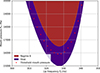 |
Figure 10 Zoom of Figure 8 around regime 6 (in brown) together with "Slow" regime (purple) and theoretical mouth pressure threshold (dotted red line). |
To reduce the computation time, a solution of the model (6) is labelled "Slow" if the signal envelope logarithmic slope is “too far” from 0 even after a fixed simulation time of 20 s. However, for lip parameters close to the boundary between two regimes, the solution may converge increasingly slowly toward one or the other regime, which induces a small logarithmic slope. This is clearly seen in Figure 10 where an enlargement of Figure 8 is shown after a new and refined computation of the regimes given by the listing Algorithm 6. Note that the neighbours of interest are specified so that no time is allocated to couples of classes that are not neighbours.
bounds = [[300, 14e3], [350, 2e4]]
neighbours = [["Silent", "Slow"], ["6", "Slow"]]
clf = edsd.edsd(beta, X0=[], bounds=bounds,
processes=16, N0 = 200, N1 = 3000,
svc=dict(C = 1e4), neighbours = neighbours)
As expected, we see that the destabilization threshold of the static regime lies within the "Slow" area.
3.6 Case of ℂ-representation
Thanks to its use of a simple time integration, the pyEDSD library can shed a new light on the use of ℂ and ℝ-representations of the impedance.
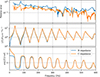 |
Figure 11 Comparison between ℂ-reprensetation (orange curves) and ℝ-representation (blue curves) of the input impedance of a Courtois trombone: relative error (top panel) with respect to the experimental data, modulus (middle panel) and argument (bottom panel). |
Figure 11 shows both impedance representations of a Courtois trombone, obtained experimentally in [6]. The top panel shows the relative errors of both representations, showing that the ℂ-impedance fits better the experimental data. This is expected since it has more degrees of freedom than the ℝ-representation. The second panel in Figure 11 shows the reconstructed impedances magnitude. It shows that the ℂ-representation is non zero for zero frequency. Moreover, as the third panel shows through a display of the phase of both impedance representations, the ℂ-representation is not even passive. This fact alone suggests that the model should behave badly, and the goal of this section is to show that this problem can be circumvented for large enough values of the lip frequency.
The RK4 numerical scheme appears to be unstable when computing some solutions, so it is replaced in this section by a trapezoidal rule solver, which gives good approximations of constant Lyapunov stable solutions. The trapezoidal rule solver is implicit and is consequently slower than the RK4 scheme. Moreover, “ovr” strategy is used to determine the regimes boundaries, as detailed in Algorithm 7.
bounds = [[0, 0], [350, 2e4]]
X0 = [[f, 18e3]
for f in np.linspace(10, 350, 10)]
X0 += [[50, 160]]
for n in ["1", "2", "3", "4", "5", "6", "Nan"]:
def f(x) :
return(func(x) == n)
clf = edsd.edsd(f, X0=X0, bounds=bounds,
processes=16, N0 = 10, N1 = 500,
svc=dict(C = 1000)) #
edsd.save(clf, f"carte_multiC-{n}-ovr.edsd")
The output of pyEDSD is shown in Figure 12. The different regimes are represented by colour patches, and are superimposed with the boundaries of regimes obtained with the ℝ-representation already shown in Figure 8, and represented here by black lines.
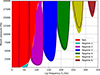 |
Figure 12 Regimes obtained by pyEDSD for the ℝ-representation of impedance (black lines) and ℂ-representation (coloured patches). |
In this figure, there is a noticeable but relatively small difference between regimes 3 to 6 obtained with the two types of representations, but the other regimes are completely disrupted by the ℂ-representation, to such an extent that regime 1 almost entirely disappears and is replaced by the "Nan" regime which corresponds to downstream pressure with a RMS value above a non physical level.
To explain this phenomenon, a point in the "Nan" regime is chosen and the solution given by the trapezoidal rule solver is shown in Figure 13, where it appears to converge toward a constant negative solution.
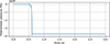 |
Figure 13 Convergence toward a non zero solution obtained with the trapezoidal rule solver starting at zero. |
These solutions are actually known at least since the work of Velut [5] where it was shown that, in the case of ℂ-representation, there are three different equilibrium solutions, all with non zero amplitude: one with small amplitude, and the other two that have no physical interpretation. Figure 13 shows that at least one of these non realistic solutions is actually Lyapunov stable. Moreover, Figure 12 shows that the solution of (6) initialised with Ξ0 tends toward a non physical solution for a large range of small lip frequency. This is consistent with the fact that, for sufficiently small lip frequency values, the model obtained using ℂ-representation is not passive.
From now on, we will only focus on theℝ-representation of the impedance.
3.7 Generalisation to 3D
We can now turn to the production of regime cartography when H, p m and F ℓ vary, while Q ℓ and μ are kept fixed to the values given in Table 1. These three parameters have been chosen because their effects have already been studied (cf. [6]).
 |
Figure 14 Boundary or the regimes regions obtained by pyEDSD as functions of the lip frequency, mouth pressure and opening at rest as detailed in program Algorithm 8, colour legends as in Figure 8. |
Figure 14 represents the result of the Algorithm 8 (computation time: 6 min), obtained with pyEDSD using the “ovo” strategy for H varying in the range [ − 10−2 m, 10−2 m]. The need for negative valued H comes from personal experiments as it appears necessary in some cases to produce low notes. This is made possible because the lips opening is allowed to be negative in the model (6), and can be interpreted as tight lips.
bounds = [[20, 10, -1e-2], [350, 25e3, 1e-2]]
X0 = [[f, 15e3, 0]
for f in np.linspace(360, 390, 5)]
neighbours = [[str(i), str(i+1)]
for i in range(len(regimes)+3)]
neighbours += [["Silent", str(i)]
for i in range(len(regimes))]
clf = edsd.edsd(func, X0=X0, bounds=bounds,
processes=16, classes = 16, N0 = 1000,
N1 = 6000, svc=dict(C = 1000),
neighbours = neighbours)
edsd.save(clf, "carte_multi_3d.edsd")
The set of neighbours considered are the same as that in Figure 8, the regimes "Nan" and "Slow" are not computed.
For an interactive version of this three-dimensional figure, see the https://perso.univ-lemans.fr/smauge/Acoustics/pyEDSD/cartemulti3d.html plotted with the plotly.js.
3.8 Comparing 2D and 3D
Each classifier produced by the pyEDSD library has a restriction method that produces a new classifier defined via a map. It can be used either as a proper restriction, or as a way to reduce the region of interest. The restriction method takes as argument a new cuboid C′, and a function C′ into C. For example, loading the 3D classifier from the previous section and restricting H (i.e. the third argument) to H = 0.5 mm is done as in Algorithm 9. This new classifier can be displayed and compared to that of Figure 8. This comparison is shown in Figure 15 where colour patches represent the restricted classifier, and the black lines the contours of the original 2D classifier.
clf = edsd.load("carte_multi_3d.edsd")
clf.restriction([[0, 0], [350, 25000]],
lambda x:[x[0], x[1], 5e-4])
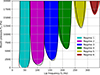 |
Figure 15 Comparison of the 2D classifier of Section 3.3 (black lines), and the 3D classifier of Section 3.7 (colour patches) restricted to H = 0.5 mm. |
The result is satisfactory, although a difference is clearly present, albeit less critical than that introduced by a ℂ-representation of the impedance (see Fig. 12). The discrepancy between both methods may come from different sources:
-
the resolution used during the computation of classifiers (which could be increased by changing N 1);
-
the choice of kernel used for the classifications. Here the default “rbf” was chosen, as it appears to be a good choice in many situations;
-
the parameters used during the SVM to change the kernel regularity (parameters C and γ of the scikit-learn function svm.SVC), as these parameters ensure the classifier smoothness, and are used to correct some artefact that may appear.
3.9 Application to the ease of play
According to [4], Section 5.2.2, cartographies like that of Figure 8 are useful to study the ease of playing, as they give information about the mouth pressure threshold necessary to produce a sound for a given regime.
In this section, the objective is to investigate the influence of lip opening at rest and lip frequency on the ease of playing. To do so, restrictions of the 3D classifier are used to study the evolution of maximal parameter ranges when a quantity varies. As an example, let us fix pm = 15 kPa and draw the corresponding restricted classifiers as in Figure 16. The boundingbox method of each classifier is then used to estimate the range of each parameter for a given regime. This bounding box is computed using a Monte-Carlo method to produce boundary points, as detailed in Section 2.6. An example is shown as red rectangles in Figure 16 for regimes 3 to 6.
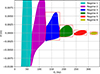 |
Figure 16 Restriction to p m = 15 kPa of the 3D classifier shown in Figure 14, together with bounding boxes (red rectangles) obtained by a Monte-Carlo method. |
With this technique, it is possible to follow the evolution of playing frequency and opening at rest ranges with respect to a change in mouth pressure, as detailed in the Algorithm 10.
clf = edsd.load("carte_multi_3d.edsd")
N = ["1", "2", "3", "4", "5", "6"]
P = np.linspace(1e3, 2e4, 20)
H = [[] for n in N]
F = [[] for n in N]
for p in P:
def res(x) :
return([x[0], p, x[1]])
restricted_clf = clf.restriction(
[[0, -1.5e-2], [350, 1e-2]], res)
for n in N :
restricted_clf.reset_random_pool()
b=restricted_clf.boundingbox(size_random = 200,
class_id = str(2+n), processes = 16)
F[n].append(b[1][0]-b[0][0])
H[n].append(b[1][1]-b[0][1])
Figure 17 shows the evolution of relative ranges of lip frequency and opening at rest for which each periodic regime from "1" to "6". Note that by construction, ΔH is bounded by 2 cm.
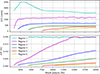 |
Figure 17 Evolutions of relative ranges of lip frequency (top, in cents) and opening at rest (bottom, in percentage) with respect to p m . |
Except for the first regime, Figure 17 shows that both lip frequency and opening at rest ranges increase with mouth pressure, which means that the precision in F ℓ and H is less critical to produce a sound at higherpressure.
4 Conclusion
We presented pyEDSD, an open-source python toolbox that implements an Explicit Design Space Decomposition (EDSD) method based on support vector machines (SVM). The toolbox is designed to construct boundaries in the space of relevant quantities of the model such as parameters or initial conditions. It was used as a tool to separate regions corresponding to different behaviors, e.g. distinct oscillation regimes.
The toolbox capabilities have been illustrated in details in simple examples, and the performances of the toolbox in terms of both the accuracy of the results and the computation time have been assessed. In particular, a comparison between the different possible strategies to handle classification between multiple classes (regimes) is provided.
The possibilities of the toolbox have been subsequently illustrated on a model of an actual physical system, namely a trombone model with 11 resonance modes written as a set of 24 coupled ordinary differential equations. This system is known to produce several periodic regimes (corresponding to musical notes) with different oscillation frequency depending on the main control parameters. Importantly, several stable regimes can coexist in some parameter regions, in a multistable configuration.
In the space of relevant control parameters, for a given set of initial conditions corresponding to silence (i.e. no oscillation) and for two different formulations of the model, we computed cartographies showing which regime is observed when a step of the blowing pressure, taken here as a prototypical attack transient of the musician, is performed. Our results illustrate that this approach is complementary to other approaches, in particular numerical bifurcation analysis. In particular, the method is well suited for the exploration of high-dimensional space of parameters, or other relevant quantities. Importantly, cartographies can be obtained in spaces of different kind of quantities, for example a control parameter and a set of initial conditions, thus leading to the simultaneous investigation of the bifurcation structure of the system as well as of its basins of attraction. Finally, and although we focused here on distinguishing between different dynamical regimes, it is important to note that any kind of classification criterion can be set by the user, e.g. amplitude, frequency, spectral content, etc. From an application point of view, this can be particularly valuable in the context of assistance to musical instrument design, for example to determine the design parameters leading to an enhanced playability or to an improved intonation of the instrument.
CODES is available at http://codes.arizona.edu/toolbox/.
Acknowledgments
The authors would like to thank Youssef Esstafa for his advices on SVM.
Conflicts of interest
The code for pyEDSD and the data for this article are available at pyEDSD’s Github at https://github.com/Maugeais/pyEDSD. The data are available from the corresponding author on request.
Data availability statement
The authors declare that they have no conflicts of interest.
References
- T. Colinot, C. Vergez, P. Guillemain, J.B. Doc: Multistability of saxophone oscillation regimes and its influence on sound production. Acta Acustica 5 (2021) 33. [CrossRef] [EDP Sciences] [Google Scholar]
- R. Mattéoli, J. Gilbert, S. Terrien, J.P. Dalmont, C. Vergez, S. Maugeais, E. Brasseur: Diversity of ghost notes in tubas, euphoniums and saxhorns. Acta Acustica 6 (2022) 32. [CrossRef] [EDP Sciences] [Google Scholar]
- S. Terrien, C. Vergez, B. Fabre, P. de la Cuadra: Emergence of quasiperiodic regimes in a neutral delay model of flute-like instruments: influence of the detuning between resonance frequencies. Journal of Computational Dynamics 9, 3 (2022) 465–482. [Google Scholar]
- M. Campbell, J. Gilbert, A. Myers: The Science of Brass Instruments. Springer-Verlag, 2021. [Google Scholar]
- L. Velut, C. Vergez, J. Gilbert, M. Djahanbani: How well can linear stability analysis predict the behaviour of an outward-striking valve brass instrument model? Acta Acustica United with Acustica 103, 1 (2017) 132–148. [CrossRef] [Google Scholar]
- R. Mattéoli, J. Gilbert, C. Vergez, J.P. Dalmont, S. Maugeais, T. Soizic, F. Ablitzer: Minimal blowing pressure allowing periodic oscillations in a model of bass brass instruments. Acta Acustica 5 (2021) 57. [CrossRef] [EDP Sciences] [Google Scholar]
- J.S. Cullen, J. Gilbert, D.M. Campbell: Brass instruments: linear stability analysis and experiments with an artificial mouth. Acta Acustica United with Acustica 86, 4 (2000) 704–724. [Google Scholar]
- V. Fréour, L. Guillot, H. Masuda, S. Usa, E. Tominaga, Y. Tohgi, C. Vergez, B. Cochelin: Numerical continuation of a physical model of brass instruments: application to trumpet comparisons. The Journal of the Acoustical Society of America 148, 2 (2020) 748–758. [CrossRef] [PubMed] [Google Scholar]
- S. Maugeais, J. Gilbert: Brass players mask parameters obtained by inverse method. Acta Acustica 7 (2023) 28. [Google Scholar]
- B. Krauskopf, Hinke M. Osinga, J. Galán-Vioque, eds. Numerical Continuation Methods for Dynamical Systems: Path Following and Boundary Value Problems. Understanding Complex Systems. Springer Netherlands, Dordrecht, 2007. [Google Scholar]
- A. Basudhar, S. Missoum, A. Harrison Sanchez: Limit state function identification using Support Vector Machines for discontinuous responses and disjoint failure domain. Probabilistic Engineering Mechanics 12 (2008) 1–11. [Google Scholar]
- A. Basudhar and S. Missoum: Adaptive explicit decision functions for probabilistic design and optimization using support vector machines. Computers and Structures 86 (2008) 1904–1917. [Google Scholar]
- A. Basudhar and S. Missoum: A sampling based approach for probabilistic design with random fields. Computer Methods in Applied Mechanics and Engineering 198 (2009) 3647–3655. [Google Scholar]
- A. Basudhar and S. Missoum: An improved adaptive sampling scheme for the construction of explicit boundaries. Structural and Multidisciplinary Optimization 42 (2010) 517–529. [Google Scholar]
- A. Basudhar, C. Dribusch, S. Lacaze, S. Missoum: Constrained efficient global optimization with support vector machines. Structural and Multidisciplinary Optimization 46 (2012) 201–221. [Google Scholar]
- S. Lacaze and S. Missoum: A generalized “max-min” sample for surrogate update. Structural and Multidisciplinary Optimization 49, 4 (2014) 683–687. [Google Scholar]
- S. Missoum, C. Vergez, J.B. Doc: Explicit mapping of acoustic regimes for wind instruments. Journal of Sound and Vibration 333, 20 (2014) 5018–5029. [Google Scholar]
- J.-B. Doc, C. Vergez, S. Missoum: A minimal model of a single-reed instrument producing quasi-periodic sounds. Acta Acustica United with Acustica 100, 3 (2014) 543–554. [Google Scholar]
- T. Colinot, N. Szwarcberg, C. Vergez, S. Missoum: Cartography of a multistable system using support vector machines, applied to a clarinet model. Nonlinear Dynamics 113, 11 (2025) 13031–13042. [Google Scholar]
- V.N. Vapnik: Pattern recognition using generalized portrait method. Automation and Remote Control 24 (1963) 774–780. [Google Scholar]
- B.E. Boser, I.M. Guyon, V.N. Vapnik: A training algorithm for optimal margin classifiers, in: Proceedings of the Fifth Annual Workshop on Computational Learning Theory. COLT’92. Association for Computing Machinery, Pittsburgh, Pennsylvania, USA, 1992, pp. 144–152. [Google Scholar]
- V.N. Vapnik: The Nature of Statistical Learning Theory. Springer-Verlag New York, Inc., 1995. [Google Scholar]
- N. Cristianini, J. Shawe-Taylor: An Introduction to Support Vector Machines and Other Kernel-based Learning Methods. Cambridge University Press, 2000. [Google Scholar]
- F. Pedregosa, G. Varoquaux, A. Gramfort, V. Michel, B. Thirion, O. Grisel, M. Blondel, P. Prettenhofer, R. Weiss, V. Dubourg, J. Vanderplas, A. Passos, D. Cournapeau, M. Brucher, M. Perrot, E. Duchesnay: Scikit-learn: machine learning in python. Journal of Machine Learning Research 12 (2011) 2825–2830. [Google Scholar]
- D.J. Ewins: Modal Testing: Theory, Practice and Application, 2nd edn. Wiley, 2009. [Google Scholar]
- A. Chaigne, J. Kergomard: Acoustics of Musical Instruments. Modern Acoustics and Signal Processing. Springer, New York, NY, 2016. [Google Scholar]
- F. Ablitzer: Peak-picking identification technique for modal expansion of input impedance of brass instruments. Acta Acustica 5 (2021) 53. [CrossRef] [EDP Sciences] [Google Scholar]
- A. de Cheveigné, H. Kawahara: YIN, a fundamental frequency estimator for speech and music. The Journal of the Acoustical Society of America 111, 4 (2002) 1917–1930. [CrossRef] [PubMed] [Google Scholar]
- J.S. Elliott: Non-linear regeneration mechanisms in wind instruments. Le Journal de Physique Colloques 40, C8 (1979) C8-341. [Google Scholar]
- E.J. Doedel: AUTO-07P, Continuation and Bifurcation Software for Ordinary Differential Equations. Ver. 0.9.3, https://github.com/auto-07p/auto-07p. [Google Scholar]
Cite this article as: Maugeais S. & Terrien S. 2025. Cartography of a trombone sound regimes using a python implementation of a Support Vector Machine-based Explicit Design Space Decomposition. Acta Acustica, 9, 63. https://doi.org/10.1051/aacus/2025038.
All Tables
Frequencies of the first seven input impedance peaks of a Courtois T149 trombone fitted with a bass trombone mouthpiece Holton 181. The first row indicates the peak number.
All Figures
|
Figure 1 Theoretical example of a SVM in the square [0, 1]2 obtained with scikit-learn. The left panel is linear, the right panel is radial. The labels are represented by different colours, red and blue. The cyan curve represents the separation between regions associated to different labels. The yellow and purple curves represent the limits of the specified margins around the boundary. |
| In the text | |
|
Figure 2 Example of a multi-class SVM. A posteriori, the boundary in the middle could have been discarded, see Section 2.5. |
| In the text | |
|
Figure 3 Example of random points created on the boundary of an SVM. For this example, all points verify |D(x i )| < 7.10−8. |
| In the text | |
|
Figure 4 Evolution of the relative error in the estimation of the diameter (circles) of the trifolium as represented in Figure 3, and corresponding computation time (crosses) with the number of points on the boundary. Cyan and purple colors correspond to the case of one and 20 workers respectively. |
| In the text | |
|
Figure 5 Example of a SVM constructed with Algorithm 1 and a mesh obtained with the method described in Section 2.6. The bounding box is also computed using the boundary points. |
| In the text | |
|
Figure 6 Periodic part of signal obtained from system (6) with ℝ-decomposition of the input impedance, mouth pressure pm = 6000 Pa, lip parameters from Table 1 and 3 different lip frequencies Fℓ. |
| In the text | |
|
Figure 7 Evolution of the playing frequency with respect to lip frequency, obtained with Algorithm 4 for each lip frequency and initial condition Ξ0. The lip parameters are those of Table 1, the mouth pressure is pm = 6000 Pa and the program uses a ℝ-representation of the input impedance. |
| In the text | |
|
Figure 8 Map of regimes 1 to 6 obtained with pyEDSD, together with theoretical pressure threshold as a red dotted line obtained with auto-07p. |
| In the text | |
|
Figure 9 Bifurcation diagrams representing the evolution of root mean square value of the downstream pressure p with respect to the mouth pressure pm, for the lip parameters of Table 1 and two different values of the lip frequency: Fℓ = 101.8 Hz (blue curve) and Fℓ = 93.2 Hz (green curves). Stable and unstable parts of the branches are represented by solid and dashed lines, respectively. The pressure threshold is indicated in each case by a red circle. |
| In the text | |
|
Figure 10 Zoom of Figure 8 around regime 6 (in brown) together with "Slow" regime (purple) and theoretical mouth pressure threshold (dotted red line). |
| In the text | |
|
Figure 11 Comparison between ℂ-reprensetation (orange curves) and ℝ-representation (blue curves) of the input impedance of a Courtois trombone: relative error (top panel) with respect to the experimental data, modulus (middle panel) and argument (bottom panel). |
| In the text | |
|
Figure 12 Regimes obtained by pyEDSD for the ℝ-representation of impedance (black lines) and ℂ-representation (coloured patches). |
| In the text | |
|
Figure 13 Convergence toward a non zero solution obtained with the trapezoidal rule solver starting at zero. |
| In the text | |
|
Figure 14 Boundary or the regimes regions obtained by pyEDSD as functions of the lip frequency, mouth pressure and opening at rest as detailed in program Algorithm 8, colour legends as in Figure 8. |
| In the text | |
|
Figure 15 Comparison of the 2D classifier of Section 3.3 (black lines), and the 3D classifier of Section 3.7 (colour patches) restricted to H = 0.5 mm. |
| In the text | |
|
Figure 16 Restriction to p m = 15 kPa of the 3D classifier shown in Figure 14, together with bounding boxes (red rectangles) obtained by a Monte-Carlo method. |
| In the text | |
|
Figure 17 Evolutions of relative ranges of lip frequency (top, in cents) and opening at rest (bottom, in percentage) with respect to p m . |
| In the text | |
Current usage metrics show cumulative count of Article Views (full-text article views including HTML views, PDF and ePub downloads, according to the available data) and Abstracts Views on Vision4Press platform.
Data correspond to usage on the plateform after 2015. The current usage metrics is available 48-96 hours after online publication and is updated daily on week days.
Initial download of the metrics may take a while.