| Issue |
Acta Acust.
Volume 9, 2025
|
|
|---|---|---|
| Article Number | 71 | |
| Number of page(s) | 9 | |
| Section | Musical Acoustics | |
| DOI | https://doi.org/10.1051/aacus/2025058 | |
| Published online | 25 November 2025 | |
Technical & Applied Article
Comparing classical and empirical end correction models using spatial pressure measurements in flue pipes
1
Rollins College, Department of Physics, Winter Park, FL, 32807, USA
2
High Point University, Department of Physics, High Point, NC, 27262, USA
* Corresponding author: This email address is being protected from spambots. You need JavaScript enabled to view it.
Received:
4
September
2025
Accepted:
17
October
2025
Abstract
This study evaluates end-correction behavior in flue organ pipes by comparing two models: the classical low-frequency expression of Levine and Schwinger and the empirical, frequency-dependent refinement of Davies et al. [Journal of Sound Vibration 72 (1980) 543–546], later revisited by Moore et al. [JASA Express Letters 3 (2023) 055002]. Using a Microflown probe, we performed high-resolution pressure measurements inside and outside circular and square pipes to capture the transition from standing-wave to radiating behavior. Sinusoidal variation within the end-correction region and 1/r decay beyond were observed, consistent with theory. A two-region curve-fitting approach quantified each model’s accuracy. In the tested range (0.049 ≤ ka ≤ 0.377), both models reproduced the data with nearly identical accuracy (R2 ≥ 0.997), with only a slight advantage for the classical form in one square-pipe case. Probe interference was evaluated and found negligible. While the analysis employs fixed end-correction values rather than a universal fit, it provides a controlled test of how well existing models capture the spatial pressure field near the pipe termination. Results indicate that both models are adequate in this regime, and that the radiating field beyond δ follows a robust 1/r decay independent of model choice.
Key words: End correction / Flue organ pipe / Waveguide acoustics
© The Author(s), Published by EDP Sciences, 2025
 This is an Open Access article distributed under the terms of the Creative Commons Attribution License (https://creativecommons.org/licenses/by/4.0), which permits unrestricted use, distribution, and reproduction in any medium, provided the original work is properly cited.
1 Introduction
Flue organ pipes offer a well-defined system for studying waveguide acoustics: a reed-less mouth excites an open–open resonator with simple geometry but complex boundary behavior. Because the pressure node at an open termination lies just outside the physical end, the pipe behaves as if it were longer by an end-correction distance δ. For low frequencies, Levine and Schwinger’s diffraction analysis predicts an end correction of,
 (1)
(1)
where a is the radius of a pipe with circular cross-section. This expression is widely accepted and forms the basis for most theoretical and applied models in musical acoustics and duct acoustics [1]. Although the concept of end correction was extended to rectangular organ pipes in early experimental work [2], and has since appeared in various flow and impedance studies [3, 4], systematic validation of end-correction models has focused primarily on circular geometries.
Despite its widespread use, the classical end-correction model is rarely validated using spatially resolved pressure measurements. Most experimental studies rely on global resonance frequency measurements or impedance-based techniques. Optical experiments by Moore et al. using transmission electronic speckle pattern interferometry (TESPI) offered rare spatial insight but revealed an unexpected pressure node inside the pipe and reported an exponential, rather than sinusoidal, pressure decay for k a ≤ 1 [3]. To better match their observed nodal location, Moore et al. revisits an empirical refinement to the end correction, proposed by Davies et al. [5],
![Mathematical equation: $$ \begin{aligned} \delta _m = a \mathopen \mathclose {\left(0.6133 - 0.1168\,[{ka}]^2\right)}, \end{aligned} $$](/articles/aacus/full_html/2025/01/aacus250133/aacus250133-eq2.gif) (2)
(2)
which introduces a frequency-dependent correction term not found in the original Levine and Schwinger analysis.
Davies et al. [5] introduced the empirical quadratic refinement in equation (2) based on their measurements of reflection coefficients in flow ducts. Their method inferred end correction indirectly from wave decomposition inside the tube, focusing on how subsonic flow alters reflection magnitude without directly mapping the near-field pressure. In contrast, the present work examines the axial pressure distribution both inside and outside the pipe, providing spatially resolved validation of end-correction models. We note, however, that unlike TESPI, our approach necessarily places a physical probe within the acoustic field, which raises the possibility of perturbing the standing-wave structure. Careful assessment of this potential interference is therefore included in our methodology to ensure that any probe effects remain negligible.
While this empirical form, equation (2), aligns with TESPI data at moderate k a, it has not been tested using pointwise pressure measurements. Moreover, spatial discrepancies in nodal structure and wave decay observed in prior optical studies raised questions about how well either model reflects the true acoustic pressure behavior in and around the pipe. Other studies, such as those by Rucz et al. [6] and Hruška et al. [7, 8], have explored mouth behavior and reflection coefficients, but without resolving the axial pressure distribution in the end-correction region.
To address this gap, we conducted direct, spatially resolved pressure measurements using a Microflown probe mounted on a translation stage. This setup enabled high-resolution scans inside and outside circular and square flue pipes in the low-k a regime (0.049 ≤ k a ≤ 0.377) using the same geometric configuration as Moore et al. We fit sinusoidal (inside) and radiative (1/r) (outside) pressure models to the measured data and compare the results using two candidate values of δ: the classical value from Levine and Schwinger, and the empirical refinement in equation (2). By computing the sum of squared errors (SSE) in each case, we assess which model more accurately reflects the observed spatial pressure behavior in each region.
These measurements allow us to test several key aspects of end-correction behavior. Specifically, we evaluate (i) whether the axial pressure envelope inside the pipe follows a sinusoidal standing-wave form, (ii) whether the radiated field beyond the pipe exhibits 1/r decay, (iii) whether an internal node appears near the pipe end, as previously reported in optical studies [3], and (iv) which candidate end correction – classical or empirical – more accurately describes the spatial domain based on fit quality. Together, these results provide practical validation of end-correction models and offer insight into wave behavior near pipe terminations in the low-to-moderate ka regime, with implications for musical acoustics, waveguide modeling, and aeroacoustic analysis.
While the present work compares two established end-correction models using fixed δ values, we do not attempt a universal fit or frequency-dependent reformulation of δ beyond those expressions. Developing a generalized δ(k a) relationship would require extending the parameter space to higher frequencies, wall geometries, and flow conditions than considered here. Such an analysis, though potentially valuable for future studies, lies outside the scope of this experiment, which is focused on spatially resolved validation of existing models in the low-k a-pagination regime.
2 Methods
2.1 Experimental setup
The mouthpiece (including the fipple) of each flue organ pipe was designed in Rhino 7 (Robert McNeel and Associates, Seattle, WA) and produced using a MakerBot Replicator+ 3D printer (MakerBot Industries, Brooklyn, New York, USA). To match the experiments of Moore et al., prefabricated plexiglass tubes with circular or square cross sections were attached to each printed mouthpiece to form the full-length resonator. This configuration enabled direct comparison between optical and acoustic measurement methods. The selected geometries and frequency ranges (0.049 ≤ ka ≤ 0.377) ensured operation in the plane-wave regime while spanning the range where deviations from classical end-correction behavior were previously observed. Prior studies have shown that wall thickness can affect the radiated field near an open pipe, particularly through its influence on diffraction and the effective end correction [4]. To control for this, all attached pipes in our study had thin, uniform walls and sharp edges. The cylindrical assembly used a 0.48 m long plexiglass tube with an inner radius of 0.01 m, while the square assembly used a 0.36 m long plexiglass tube with a 0.01 m side length. A compressed-air source drove each pipe, and measurements were taken at different resonant frequencies to capture behavior at both low and high harmonics. Specifically, the circular pipe was excited at its third harmonic (approximately 870 Hz) and seventh harmonic (approximately 2056 Hz), while the square pipe was excited at its first harmonic (approximately 474 Hz) and second harmonic (approximately 875 Hz). These choices aligned with the mostly reliably playable harmonics for each geometry and allowed for direct comparison with prior work. As a result, two frequencies were tested per geometry.
A zero-degree sound-intensity probe (PU Match, Microflown Technologies, Arnhem, Netherlands) was used to measure acoustic pressure in the region just inside and immediately outside the pipe’s open end, where the end-correction effect is expected to occur [10]. The probe’s compact dimensions (58.7 mm length, 7 mm diameter) minimize disturbance to the acoustic field. Although the sensor can record both particle velocity and pressure, only the pressure channel was analyzed in this study. The probe was mounted on an optical table atop a horizontal translation stage for precise, repeatable positioning along the pipe’s central axis. For each trial, measurements were taken at 181 discrete positions, spaced 0.127 mm (0.005 in) apart, covering a total scan range of 22.86 mm, from 2.54 mm inside the physical end of the pipe to 20.32 mm outside. The inner boundary was set by the physical travel limit of the manual translation stage, which also defined the step size. This configuration allowed precise and repeatable positioning along the pipe axis while capturing both the standing-wave and radiating-wave regions with sub-millimeter resolution. Each pressure signal was sampled for 23 ms at 44.1 kHz, providing sufficient temporal resolution to capture the oscillatory acoustic field. A flowmeter monitored the blowing pressure to maintain consistent flow conditions throughout each sweep and reduce inter-trial variability. For each frequency condition, the blowing pressure was held constant across repeated trials to ensure stable excitation, although the absolute blowing pressure was not identical between frequencies. This choice reflects the practical operation range of each pipe and does not affect the fitted end-correction behavior, which depends on geometry and ka rather than excitation amplitude in the linear regime. Three trials were conducted for each frequency of interest and the point-by-point data were averaged. The complete measurement apparatus is illustrated in Figure 1.
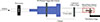 |
Figure 1. Diagram of the experimental apparatus. 3D printed organ pipe bodies with pipes of circular or square cross-section are driven by a compressed air source (from the left). Measurements of the end of the pipe were made using a Microflown sensor on a horizontal translation stage. Adapted from Schefter et al., not to scale [9]. |
At each of the 181 positions, the raw pressure–time waveform was recorded as an uncalibrated voltage in LabVIEW. A custom MATLAB script then computed the root-mean-square (RMS) value of each 23 ms waveform, reducing the time series to a single representative pressure magnitude at each location. These RMS values, expressed in arbitrary units, were plotted vs. distance from the pipe’s physical end (in millimeters). Two examples of the raw pressure–time data (blue) and their corresponding normalized RMS values (black) are shown in Figure 2. In Figure 2, the dashed grey line indicates the physical end of the pipe at zero distance, while the solid gray line marks the theoretical end-correction distance (δ) calculated from the measured frequency and pipe radius using equation (2). Using equation (1) did not produce any noticeable change in the position of the gray line on the graph. The RMS pressure values were normalized to facilitate comparison across trials and with theoretical models. This normalized RMS pressure distribution provides the basis for the curve fitting and model evaluation presented in the next section, allowing direct comparison between the observed end-correction behavior (sinusoidal standing wave) and the expected radial decay (1/r) beyond the end-correction region.
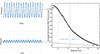 |
Figure 2. Raw data points recorded as pressure vs. time (blue scatter plots on left) represented as a point on the graph as a normalized RMS pressure from a distance from the physical end of the pipe in mm. The dashed, gray line represents the physical end of the pipe at zero and the solid gray line represents the end correction (δ) calculated from the measured frequency and the radius of the pipe using equation (2). The data to the left of δ are fit to a sinusoidal function, consistent with end-correction theory, which assumes a standing wave in this region. Beyond δ, where the wave is propagating, the data are fit to a 1/r function. |
2.2 Assessment of sensor interference
Because the Microflown pressure probe has a diameter of 7 mm [10] (compared to the 20 mm pipe diameter), we investigated how inserting it affects the standing-wave frequency. With the circular pipe at a fixed blowing pressure, we used the Microflown sensor to record the resonant pitch as the probe moved from 17.0 mm inside the bore to just outside, stepping in 0.127 mm increments. Over this 17.0 mm span, the observed frequency shifted by up to 1.5 Hz in the circular pipe. A similar test in the square pipe (22.9 mm range) showed a 2.5 Hz shift. This slight difference is likely due to the larger percentage change in the effective length for the shorter square pipe (0.36 m) compared to the longer cylindrical pipe (0.48 m). The shorter 17 mm span for the circular-pipe interference check was sufficient to capture the in-pipe region where frequency sensitivity is greatest; all main measurement scans used the full 22.86 mm range described in Section 2.1.
To assess whether small frequency drifts could impact the calculated end correction δ, we apply Moore’s empirical δ
m
, equation (2) with  . For a pipe of radius a = 0.01 m, driven near 870 Hz with sound speed c = 343 m/s, the nominal end correction is δ(870 HZ) ≈ 6.10336 mm. If the frequency shifts by 1.5 Hz or 2.5 Hz during scanning, the corresponding changes in end correction are:


These correspond to relative changes of 0.002% and 0.004% in δ, respectively. Compared to our spatial sampling interval of 0.127 mm, the deviations represent less than 0.2% of a single step. We therefore conclude that frequency drift on the order of 1–2 Hz has a negligible effect on the fitted end correction and does not influence which points are classified as inside or outside the end-correction region.
Beyond frequency drift, we estimated an upper bound for geometric blockage by treating the probe tip as a solid disc of radius r
p
= 3.5 mm in a circular pipe of radius R = 10 mm, yielding an area fraction ε = (r
p
/R)2 ≈ 0.1225 (12.25%). The corresponding effective radius scales as  , implying a 6% decrease in a and in δ, or a 0.36 mm reduction in end correction for the circular pipe. Such a change would shift the resonance frequency by roughly 1 Hz – consistent with the small drift observed – and would produce a noticeable fit mismatch if larger. In practice, the PU-Match tip is annular rather than solid, so the actual blockage is smaller. Combined with the negligible frequency sensitivity reported above, these results confirm that probe presence does not measurably bias the fitted end correction under the present conditions.
2.3 Data analysis with curve fitting
To characterize the spatial pressure distribution near the open end of the pipe, we apply a two-region fitting model that reflects idealized expectations in waveguide acoustics. Inside the pipe, up to an acoustical length δ beyond the physical end (x = 0), the pressure is modeled as a standing wave. Beyond δ, the field transitions to an outwardly radiating wave. Although the existence of a sharply defined boundary between these regimes is an approximation, this framework enables quantitative comparison between theoretical end-correction predictions and experimental data.
For the square pipe, the Levine–Schwinger expression was applied by defining an effective radius,

where S is the cross-sectional area of the pipe. This equal-area substitution, following the approach of Moore et al. [3], equates the square aperture to a circular one of identical area and is widely used when comparing noncircular geometries. At the low ka values considered here, end correction depends primarily on aperture area rather than detailed shape, consistent with prior experimental and numerical studies [2, 11, 12]. These works collectively show that, for low ka, length corrections for square and circular apertures are nearly identical, with differences below a few percent except for slit-like shapes. Our measurements likewise show that the fitted end corrections for the square pipe closely match those of the circular pipe, confirming that aperture area is the dominant factor in this regime.
In the standing-wave region (x < δ), the normalized root-mean-square (RMS) pressure y(x) is modeled as,
 (3)
(3)
where k is the acoustic wavenumber determined from the measured resonant frequency, and A, ρ, and z are fit parameters. This sinusoidal form is consistent with idealized standing-wave behavior in open–open resonators and matches pressure profiles seen in Giordano’s Navier–Stokes simulations [13].
Beyond the acoustical end (x > δ), the pressure is modeled as
 (4)
(4)
where A and z are again fitted parameters. This form reflects the expected 1/r decay of a radiating wave from a near-field source.
To assess the accuracy of competing end-correction models, we tested two candidate values of δ: (1) the classical low-frequency expression δ LS = 0.6133a from Levine and Schwinger [1], and (2) the frequency-dependent empirical model δ m = a(0.6133 − 0.1168 [ka]2), originally proposed by Davies et al. [5] and later revisited in the optical study of Moore et al. [3]. For consistency with that more recent study, which motivated our work, we adopt the subscript m to denote the empirical model throughout this paper.
For each case, curve fits were applied separately to the standing and radiating regions using MATLAB’s Curve Fitting Toolbox. The sum of squared errors (SSE) was calculated as a measure of fit quality, with lower SSE indicating closer agreement between model and data. SSE was used for direct comparison between candidate δ values under identical model structures. The specific δ values calculated for each geometry and frequency, using both the classical and empirical models, are listed in Table 1. Differences between δLS and δm increase slightly with ka but remain under 3% across all cases. In addition to SSE, we report the coefficient of determination (R2) for each fit as a measure of absolute goodness of fit.
Computed end correction values for each pipe condition using both the classical (Levine & Schwinger) and empirical models. Differences between δ LS and δ m increase slightly with ka, but remain within 3% across all cases.
3 Results and discussion
3.1 Overview of fit results
We applied the two-region curve-fitting approach from Section 2 to evaluate how well the classical and empirical end-correction models describe the measured RMS pressure fields. To maintain an unbiased comparison between models and avoid parameter co-dependence with A, ρ, and z, we did not treat δ as a free fit parameter; instead, we held the model structure fixed and compared fits using the two established end-correction expressions. Each trial was divided into a standing-wave zone inside the pipe up to δ and a radiating-wave zone beyond δ. For each region, we fit the same functional form to the data using either δ LS = 0.6133a or δ m = a (0.6133 − 0.1168[ka]2), and compared fits using the sum of squared errors (SSE) and R 2. This allowed a direct, unbiased assessment of how well each δ separates the standing and radiating regions.
Across all trials, the RMS profiles showed a smooth transition from sinusoidal standing-wave behavior to 1/r decay, consistent with theoretical expectations. The following sections detail results for each region, with emphasis on where the models diverged.
3.2 Sinusoidal behavior inside the pipe: fitting the standing-wave region
Representative fits of the sinusoidal standing-wave model to the RMS pressure distribution inside the end-correction region are shown in Figures 3 and 4 for the circular pipe at 870 Hz and the square pipe at 875 Hz, respectively. In each plot, black points represent the measured data and the gray shaded region signifies the points excluded from the fit. The exclusion region corresponds to either inside or outside the theoretical end-correction distance (δ) calculated from the measured frequency and pipe radius using equation (2). As before, using equation (1) did not produce any noticeable change in the position of the exclusion region on the graph. Fits using both the classical δ LS (solid blue line) and empirical δ m (dashed orange line) are overlaid.
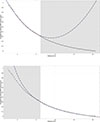 |
Figure 3. Normalized RMS pressure vs. position relative to the end of the pipe for a circular pipe at 870 Hz. Top: standing-wave (inside) fit; bottom: radiating-wave (outside) fit. The gray shading indicates points excluded from the fit and was determined using equation (2). LS (solid blue line) and empirical fits (dashed orange line) overlay closely with no visible difference, consistent with the nearly identical SSE values in Table 2. |
Sum of squared errors (SSE) and R 2 values for sinusoidal fits in the standing-wave region using δ LS and δ m . Additional columns highlight the absolute SSE difference and ratio. Only the square, high-frequency case shows a clear model difference.
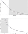 |
Figure 4. Normalized RMS pressure vs. position relative to the end of the pipe for a square pipe at 875 Hz. Top: standing-wave (inside) fit; bottom: radiating-wave (outside) fit. The gray shading indicates points excluded from the fit and was determined using equation (2). The LS fit (solid blue line) shows better phase alignment near δ inside compared to the empirical fit (dashed orange line), consistent with the lower SSE in Table 2; outside, the 1/(x + δ) decay is essentially identical for both models. |
The corresponding SSE and R 2 values for all four geometry–frequency combinations are summarized in Table 2. In three of the four cases (circular 870 Hz, circular 2056 Hz, and square 474 Hz), the fits from δ LS and δ m were visually indistinguishable and yielded nearly identical SSE values (differences < 5 × 10⁻⁴) with R 2 ≥ 0.997. Representative examples are shown in Figures 3 and 4. The only notable difference occurs for the square pipe at 875 Hz (Fig. 4), where the classical model achieves an SSE less than half that of the empirical model (0.0131 vs. 0.0274) and more closely matches the oscillation phase near the δ boundary.
Across all cases, the measured pressure envelope exhibits one smooth oscillation of sinusoidal variation up to δ, consistent with the expected open-end boundary condition. No internal node was observed in any trial, in contrast to the TESPI results of Moore et al. [3]. The strong agreement between data and sinusoidal fits supports the theoretical expectation that the standing-wave behavior extends smoothly to the end-correction point.
3.3 Radial decay outside the pipe: fitting the radiating-wave region
Beyond the end-correction distance, the measured RMS pressure profiles followed the expected 1/(x + δ) decay, consistent with spherical spreading from an unflanged pipe termination. In all cases, the measured pressure profile beyond δ formed a smooth, monotonic decay that was well captured by the radiating-wave fit.
Table 3 summarizes the SSE and R2 values for the radiating region using both δLS and δm. The fits were exceptionally good across all pipe, frequency combinations, with R2 ≥ 0.998 in every case. Differences in SSE between the two models were extremely small, typically less than 3 × 10⁻⁴.
Sum of squared errors (SSE) and R 2 values for 1/r fits in the radiating-wave region using classical and empirical end-correction values. An additional column shows the absolute SSE difference, which is negligible in all cases, even for the square, high-frequency case where standing-wave fits diverged.
Even in the square, high-frequency case (875 Hz), where the standing-wave fits in Figure 4 showed a clear difference in SSE between models, the radiating-wave fits were nearly identical (0.0274 vs. 0.027436; truncated values in Tab. 3). This indicates that once the wave has transitioned to outward radiation, the decay rate is robust against small changes in the chosen end-correction distance.
These results confirm that the radiating-field behavior is largely insensitive to δ within the tested ka range, and that both the classical and empirical models provide equally accurate predictions of the far-field decay.
3.4 Geometry and frequency effects
Geometry had little influence on model performance at low ka: both the circular (870 Hz) and square (474 Hz) cases yielded SSE < 1.3 × 10⁻³ in the standing-wave region and visually identical fits, as seen in Table 2. At higher ka, small differences emerged. For the circular pipe at 2056 Hz, SSE differences between models were minor (5 × 10⁻⁴). For the square pipe at 875 Hz, however, δ LS produced an SSE less than half that of δ m (Tab. 2), indicating slightly better phase matching in the standing-wave fit (Fig. 4).
In the radiating-wave region, geometry had no measurable effect: R 2 ≥ 0.998 for all cases and SSE differences between models were negligible (Tab. 3). The radiating-wave decay was robust to δ choice, even when standing-wave fits diverged, reinforcing the conclusion that far-field behavior is model-insensitive.
Comparing low and high ka, model agreement was strongest at low ka, where δ m is close to δ LS. At higher ka, the frequency-dependent term in δ m occasionally shifted the fitted phase enough to cause modest SSE differences, as in the square 875 Hz case. Overall, neither model consistently outperformed the other; however, δ LS retained a slight advantage at moderate ka in square pipes while performing equivalently elsewhere. The absence of an internal node across all geometries and frequencies further supports the validity of the open-end boundary condition in this ka range.
These results apply to the ka range tested (0.049 ≤ ka ≤ 0.377) and to circular and square cross-sections with sharp edges. Measurement precision was set by the 0.127 mm translation stage step size, and probe interference was shown to be negligible (Sect. 2). Extending the method to higher ka values or alternative geometries would help test the generality of these conclusions.
4 Conclusion
High-resolution, pointwise pressure measurements inside and outside circular and square flue pipes were used to directly evaluate two end-correction models: the classical, low-frequency expression of Levine and Schwinger and the empirical, frequency-dependent refinement of Moore et al. In the low-to-moderate ka range tested (0.049 ≤ ka ≤ 0.377), both models reproduced the measured standing-wave and radiating-wave behavior with high accuracy (R 2 ≥ 0.997 for all fits). Across all geometries and frequencies, the data exhibited one smooth oscillation of sinusoidal variation up to δ with no internal node, confirming the open-end boundary condition and in contrast with earlier optical observations.
In three of the four standing-wave cases, SSE differences between models were negligible. The only meaningful divergence occurred for the square pipe at moderate ka (875 Hz), where the classical model achieved an SSE less than half that of the empirical form and showed better phase alignment near the end-correction boundary. In the radiating region, both models produced nearly identical fits in all cases, with SSE differences < 3 × 10⁻⁴, indicating that far-field decay is largely insensitive to small changes in δ.
Because the empirical model includes a [ka]2 term, deviations from the classical form are expected to increase with frequency. In this study, the effect was only appreciable for the highest-ka circular case tested, but in higher-frequency applications, particularly outside the typical range for musical instruments, differences between the two models may become more significant. Future work extending this approach to higher ka values or different termination geometries would help quantify these deviations and further refine end-correction models for broader acoustic applications.
Future work could explore universal or frequency-dependent fitting of δ across a wider ka range or alternative geometries to assess whether a single formulation can describe multiple end conditions. The present results, however, suggest that within the low-ka regime, fixed-model approaches remain sufficient for capturing the relevant acoustic behavior.
Overall, these results support the continued use of the classical end correction for waveguide modeling and instrument design in the tested ka regime, while showing that either model provides equivalent predictions for far-field behavior. The measurement approach presented here offers a reproducible framework for testing and refining end-correction models in other geometries and frequency ranges.
Acknowledgments
The authors wish to thank T. Moore and N. Giordano for helpful conversations during this study.
Funding
The study was funded by National Science Foundation Award #2109932 and the Rollins College Student Faculty Collaborative Scholarship Program.
Conflicts of interest
The authors have no conflicts to disclose.
Data availability statement
Data are available on request from the authors.
Author contribution statement
L.K. Schefter conducted the investigation, data collection, analysis, and initial manuscript drafting. W.L. Coyle led the conceptualization, supervision, and methodology, and contributed to writing, editing, and funding acquisition. A.E. Cannaday supported experimental setup and methodology, and contributed to manuscript review. M. Griffin assisted with data acquisition, curation, and interpretation, and participated in manuscript review. E. Rokni contributed to experimental setup, data collection, analysis, and review.
Ethics approval
No ethical approval was required. This study was conducted in accordance with institutional policies for research and student participation.
Informed consent
This research did not involve human participants, animal subjects, or personal data.
References
- H. Levine, J. Schwinger: On the radiation of sound from an unflanged circular pipe. Physical Review 73 (1948) 383–406. [CrossRef] [Google Scholar]
- A.T. Jones: End corrections of organ pipes. The Journal of the Acoustical Society of America 12 (1941) 387–394. [Google Scholar]
- T.R. Moore, M.S. Kellison, W.L. Coyle: The behavior of standing waves near the end of an open pipe with low mean flow. JASA Express Letters 3 (2023) 055002. [Google Scholar]
- Y. Ando: On the sound radiation from a semiinfinite circular pipe of certain wall thickness. Acustica 22 (1969) 219–225. [Google Scholar]
- P.O.A.L. Davies, J.L. Bento Coelho, M. Bhattacharya: Reflection coefficients for an unflanged pipe with flow. Journal of Sound Vibration 72 (1980) 543–546. [Google Scholar]
- P. Rucz, F. Augusztinovicz, J. Angster, T. Preukschat, A. Miklós: Acoustic behavior of tuning slots of labial organ pipes. The Journal of the Acoustical Society of America 135 (2014) 3056–3065. [Google Scholar]
- V. Hruška, P. Dlask, M. Guštar: Non-destructive measurements in flue organ pipe, in: Proc. Int. Symp. Musical Acoust (ISMA). Detmold, Germany, 2019. [Google Scholar]
- V. Hruška, P. Dlask: Revisiting the open-end reflection coefficient and turbulent losses in an organ pipe. Acta Acustica 5 (2021) 47. [CrossRef] [EDP Sciences] [Google Scholar]
- L.K. Schefter, W.L. Coyle, E. Rokni, A. Cannaday: Measuring the behavior of the acoustic standing wave exiting a flue organ pipe. Proceedings of Meetings on Acoustics 54 (2024) 035005. [Google Scholar]
- Microflown Technologies: PU Match sound intensity probe. PU Probe Series. Microflown Technologies, Arnhem, The Netherlands, https://www.microflown.com/products/standard-probes/pu-match (accessed October 9, 2025). [Google Scholar]
- W. Duan, R. Kirby: A hybrid finite element approach to modeling sound radiation from circular and rectangular ducts. The Journal of the Acoustical Society of America 131 (2012) 3638–3649. [Google Scholar]
- L. Jaouen, F. Chevillotte: Length correction of 2D discontinuities or perforations at large wavelengths and for linear acoustics. Acta Acustica 104 (2018) 243–250. [Google Scholar]
- N. Giordano: Understanding end corrections and flow near the open end of a flue instrument. The Journal of the Acoustical Society of America 157 (2025) 1176–1184. [Google Scholar]
Cite this article as: Coyle W.L. Schefter L.K. Cannaday A.E. Griffin M. & Rokni E. 2025. Comparing classical and empirical end correction models using spatial pressure measurements in flue pipes. Acta Acustica, 9, 71. https://doi.org/10.1051/aacus/2025058.
All Tables
Computed end correction values for each pipe condition using both the classical (Levine & Schwinger) and empirical models. Differences between δ LS and δ m increase slightly with ka, but remain within 3% across all cases.
Sum of squared errors (SSE) and R 2 values for sinusoidal fits in the standing-wave region using δ LS and δ m . Additional columns highlight the absolute SSE difference and ratio. Only the square, high-frequency case shows a clear model difference.
Sum of squared errors (SSE) and R 2 values for 1/r fits in the radiating-wave region using classical and empirical end-correction values. An additional column shows the absolute SSE difference, which is negligible in all cases, even for the square, high-frequency case where standing-wave fits diverged.
All Figures
|
Figure 1. Diagram of the experimental apparatus. 3D printed organ pipe bodies with pipes of circular or square cross-section are driven by a compressed air source (from the left). Measurements of the end of the pipe were made using a Microflown sensor on a horizontal translation stage. Adapted from Schefter et al., not to scale [9]. |
| In the text | |
|
Figure 2. Raw data points recorded as pressure vs. time (blue scatter plots on left) represented as a point on the graph as a normalized RMS pressure from a distance from the physical end of the pipe in mm. The dashed, gray line represents the physical end of the pipe at zero and the solid gray line represents the end correction (δ) calculated from the measured frequency and the radius of the pipe using equation (2). The data to the left of δ are fit to a sinusoidal function, consistent with end-correction theory, which assumes a standing wave in this region. Beyond δ, where the wave is propagating, the data are fit to a 1/r function. |
| In the text | |
|
Figure 3. Normalized RMS pressure vs. position relative to the end of the pipe for a circular pipe at 870 Hz. Top: standing-wave (inside) fit; bottom: radiating-wave (outside) fit. The gray shading indicates points excluded from the fit and was determined using equation (2). LS (solid blue line) and empirical fits (dashed orange line) overlay closely with no visible difference, consistent with the nearly identical SSE values in Table 2. |
| In the text | |
|
Figure 4. Normalized RMS pressure vs. position relative to the end of the pipe for a square pipe at 875 Hz. Top: standing-wave (inside) fit; bottom: radiating-wave (outside) fit. The gray shading indicates points excluded from the fit and was determined using equation (2). The LS fit (solid blue line) shows better phase alignment near δ inside compared to the empirical fit (dashed orange line), consistent with the lower SSE in Table 2; outside, the 1/(x + δ) decay is essentially identical for both models. |
| In the text | |
Current usage metrics show cumulative count of Article Views (full-text article views including HTML views, PDF and ePub downloads, according to the available data) and Abstracts Views on Vision4Press platform.
Data correspond to usage on the plateform after 2015. The current usage metrics is available 48-96 hours after online publication and is updated daily on week days.
Initial download of the metrics may take a while.