| Issue |
Acta Acust.
Volume 10, 2026
|
|
|---|---|---|
| Article Number | 8 | |
| Number of page(s) | 13 | |
| Section | Ultrasonics | |
| DOI | https://doi.org/10.1051/aacus/2026004 | |
| Published online | 19 February 2026 | |
Scientific Article
A visco-thermal model for a novel type of electrostatic micromachined in-plane ultrasound transducer
1
Fraunhofer IPMS, Maria-Reiche-Str. 2, 01109, Dresden, Germany
2
Independent scholar, Goetheallee 29, 01309, Dresden, Germany
* Corresponding author: This email address is being protected from spambots. You need JavaScript enabled to view it.
Received:
3
July
2025
Accepted:
14
January
2026
Abstract
The acoustic fields within the microchannels of an in-plane electrostatic ultrasound transducer are analysed in this work by means of the Low Reduced Frequency (LRF) approximation of the Navier–Stokes equations. This device is composed primarily of two kinds of structures that can be described in rectangular coordinates – a prismatic slit and a cavity with curved walls –, for which a solution of the LRF equations is presented. The interaction between these two elements in an actual device is solved by an approximate model whereby the propagation modes are transmitted from one component to the other without energy losses. The solution of the LRF equations in the isolated components offered results that were in good agreement with equivalent finite-element simulations of the Full Linearised Navier–Stokes (FLNS) equations, whereas the approximate model of the complete structure slightly overestimates the output pressure in comparison to the corresponding simulation. The predictions of the analytic and finite-element models of the device were compared against an actual measurement, finding an approximate correspondence, although certain effects remain to be predicted by a more accurate analysis of the radiation pattern of the device.
Key words: Low Reduced Frequency / Navier–Stokes / Reduced-order modelling / Viscothermal wave propagation / L-CMUT.
© The Author(s), Published by EDP Sciences, 2026
 This is an Open Access article distributed under the terms of the Creative Commons Attribution License (https://creativecommons.org/licenses/by/4.0), which permits unrestricted use, distribution, and reproduction in any medium, provided the original work is properly cited.
1 Introduction
In-plane electrostatic ultrasound transducers – a particular kind of CMUT1 that is based on lateral motion – are microfabricated devices that emit waves by squeezing the gas in a narrow cavity between a flexible electrode (“beam”) and a static electrode (“stator”). These electrodes are carved into the depth of the chip, such that, upon electrostatic actuation, the beam is deflected in the in-plane direction whilst the gas is expelled in the out-of-plane direction, through a microslit, into the atmosphere. We have previously reported a proof of concept of this device in [1]. Figure 1 presents a scheme of said transducer, where its main components are identified: the cavity between beam and stator, the clearances that enable the motion of the beam, and the slits through which the gas is expelled. These components result in a significant damping force that determines the performance of the device near its resonance frequency. The purpose of this work is to develop analytic expressions that describe the propagation of acoustic waves in an “L-CMUT”, comparing them against finite-element simulations and experiments.
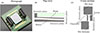 |
Figure 1. (A) Photograph of a fabricated L-CMUT and scheme of (B) its top view and (C) its cross section. The device consists of a beam that is pulled towards a stator by an electrostatic force. As this occurs, the gas in the cavity between beam and stator is expelled towards the slits and then departs from the chip, emitting ultrasound waves. |
Given that the dimensions of an L-CMUT are in the same order of magnitude as the viscous and thermal boundary layers, the application of the Full Linearised Navier–Stokes (FLNS) equations is required; nevertheless, an approximate form of these, known as the “Low Reduced Frequency” (LRF) model [2], is applicable in this case. In contrast, the applicability of the Reynolds equation is limited to low frequencies in which this device does not operate, and the classical Helmholtz wave equation does not consider the visco-thermal effects. The condition for applying the LRF approximation is that the reduced frequency be much smaller than unity, that is, k = ω l/c 0 ≪ 1. Taking a typical microslit aperture of l = 30 μm as the reference length, this requirement is met in the case of air (c = 343 m/s) up to frequencies of about 180 kHz, which is enough for the typical operation range of an L-CMUT (10–100 kHz). A direct consequence of the LRF assumption is that the pressure field in the direction of the reference length is constant. In this case of a Cartesian coordinate system, this enables a convenient separation of the cross-section coordinate (i.e. along the reference length) from the propagation coordinates. By applying the LRF equations to the geometry of an L-CMUT, we were able to develop an approximate analytical model for the prediction of the frequency-dependent damping force that is exerted onto the beam and the corresponding gas volume that is expelled from the device.
2 The LRF model for the L-CMUT
By scaling the state variables of the gas (pressure p, temperature T and density ρ) with respect to the values of the quiescent state (P
0, T
0, ρ
0) and the velocity of the particles ( ) with respect to the speed of sound (c
0), the Navier–Stokes equations can be formulated in terms of the following dimensionless variables:
) with respect to the speed of sound (c
0), the Navier–Stokes equations can be formulated in terms of the following dimensionless variables:
S2 = ɭ2ρ0ω/μ: The shear wave number squared (a Reynolds number).
k = ωɭ/c0: The reduced frequency.
σ2 = μcp/κ: The Prandtl number.
γ = cp/cv : The ratio of specific heats (adiabatic constant).
Here, μ denotes the dynamic viscosity and κ the thermal conductivity. Let the critical dimension be aligned to the y-axis (l = l
y
), leaving the the x- and z-axes for the propagation directions. The dimensionless coordinates are then  ,
,  , and
, and  . For small harmonic amplitudes at frequency ω, the LRF approximation results in the following set of linear partial differential equations for the time harmonic variations2
p
a
c
, T
a
c
, ρ
a
c
and
. For small harmonic amplitudes at frequency ω, the LRF approximation results in the following set of linear partial differential equations for the time harmonic variations2
p
a
c
, T
a
c
, ρ
a
c
and  of the normalised state variables and particle velocity, respectively:
 (1)
(1)
 (2)
(2)
 (3)
(3)
 (4)
(4)
 (5)
(5)
 (6)
(6)
The two main acoustic components of the L-CMUT structure, the beam-stator cavity and the micro-slits, are depicted in Figure 2. Let us denote the boundaries of each structure in the respective axes by  ,
,  and
and  , such that
  indicates its dimensionless thickness. The reference length for the case of the slit is denoted ly = hs, and that of the cavity is ly = g0. The major difference between the slit and the cavity is that the y-boundaries of the cavity are not plane but a function of x, turning the thickness,
  , into a function of
  as well. The
  curve of the cavity corresponds to the deflected shape of the beam, which can be calculated by a static force balance at the biasing point (see [3]), whereas the
  curve corresponds to the shape of the stator, which is freely determined by the designer. Schenk et al. [3] show why the spatial zeroth mode of a clamped-clamped Euler–Bernoulli beam (Eq. (9)) is sufficient to model very accurately the entire electrostatic bifurcation pattern of a beam under electrostatic load. This results in the general deflection profile described in equation (7), with z
DC = a
0/g
0 as the dimensionless static deflection. The arguments of [3] extend into the stiffness-dominated dynamic range relevant to this paper. Moreover, we argue in [1] that the stator profile ought to have the same shape as the beam deflection profile in order to avoid additional electrostatic instabilities. Combining these findings leads to a convenient expression for the thickness
curve corresponds to the shape of the stator, which is freely determined by the designer. Schenk et al. [3] show why the spatial zeroth mode of a clamped-clamped Euler–Bernoulli beam (Eq. (9)) is sufficient to model very accurately the entire electrostatic bifurcation pattern of a beam under electrostatic load. This results in the general deflection profile described in equation (7), with z
DC = a
0/g
0 as the dimensionless static deflection. The arguments of [3] extend into the stiffness-dominated dynamic range relevant to this paper. Moreover, we argue in [1] that the stator profile ought to have the same shape as the beam deflection profile in order to avoid additional electrostatic instabilities. Combining these findings leads to a convenient expression for the thickness  that only depends on two design variables: the static deflection (z
DC) and the stator shape factor (σ
s
).
that only depends on two design variables: the static deflection (z
DC) and the stator shape factor (σ
s
).
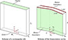 |
Figure 2. Illustration of the dimensions and coordinates used to describe the geometry of the slits and the beam-stator cavity of an L-CMUT. |
 (7)
(7)
 (8)
(8)
Here  denotes the dimensionless and normalized Euler–Bernoulli zero mode (cf. [3]) which is defined on the interval
 ![Mathematical equation: $ \xi \in \left[ -1/2,+1/2 \right] $](/articles/aacus/full_html/2026/01/aacus250087/aacus250087-eq24.gif) ,
,
 (9)
(9)
Due to the no-slip condition, we may assume a zero particle velocity component parallel to the silicon walls of the L-CMUT. The particle velocity component perpendicular to the static silicon walls vanishes because there is no mass transport across these boundaries. Likewise, we assume the silicon walls to have no temperature difference with the environment, and due to the relatively high heat capacity of the semiconductor material, that temperature fluctuations vanish at the silicon boundaries. By inserting the ansatz in equation (10) into equation (4) (as suggested in [2]), the differential equation for the profile shape function  in equation (11) emerges.
 (10)
(10)
 (11)
(11)
Similarly, inserting the ansatz in equations (12) and (13) results in a nearly identical differential equation for the profile shape function of the particle velocity,  , save for the absence of the Prandtl number (σ
2). We conclude, then, that these two functions, which are governed by differential equations with the same form and have the same boundary conditions, are identical, save for the absence of the Prandtl number in the solution of
, save for the absence of the Prandtl number (σ
2). We conclude, then, that these two functions, which are governed by differential equations with the same form and have the same boundary conditions, are identical, save for the absence of the Prandtl number in the solution of  . This coincides with the observations of Stinson [4] and Beltman [2].
 (12)
(12)
 (13)
(13)
 (14)
(14)
The solution of equation (11) for  is the cosine function in equation (15), and the solution of equation (14) for
  is the cosine function in equation (16).
![Mathematical equation: $$ \begin{aligned} C(\hat{x},\hat{y})&=\frac{\cos \left[\sqrt{\frac{s^2\sigma ^2}{j}}\left(\hat{y}-\frac{1}{2}(\hat{y}_+(\hat{x})+\hat{y}_-(\hat{x}))\right)\right]}{\cos {\left[\sqrt{\frac{s^2\sigma ^2}{j}}\frac{1}{2}\left(\hat{y}_+(\hat{x})-\hat{y}_-(\hat{x})\right)\right]}} \quad -1\end{aligned} $$](/articles/aacus/full_html/2026/01/aacus250087/aacus250087-eq36.gif) (15)
(15)
![Mathematical equation: $$ \begin{aligned} \nonumber \\ A(\hat{x},\hat{y})&=\frac{\cos \left[\sqrt{\frac{s^2}{j}}\left(\hat{y}-\frac{1}{2}(\hat{y}_+(\hat{x})+\hat{y}_-(\hat{x}))\right)\right]}{\cos {\left[\sqrt{\frac{s^2}{j}}\frac{1}{2}\left(\hat{y}_+(\hat{x})-\hat{y}_-(\hat{x})\right)\right]}}-1. \end{aligned} $$](/articles/aacus/full_html/2026/01/aacus250087/aacus250087-eq37.gif) (16)
(16)
The profile shape function for the temperature,  , also serves to calculate the density fluctuations. If equation (10) is inserted into the ideal gas equation (Eq. (5)), we obtain the following relation:
![Mathematical equation: $$ \begin{aligned} \rho _{ac}(\hat{x},\hat{y},\hat{z}) = \left[1+\left(\frac{\gamma -1}{\gamma }\right)C(\hat{x},\hat{y})\right]p_{ac}\left( \hat{x},\hat{z}\right). \end{aligned} $$](/articles/aacus/full_html/2026/01/aacus250087/aacus250087-eq39.gif) (17)
(17)
The previous results can then be incorporated into the continuity equation (Eq. (3)) to obtain a differential equation for the pressure waves:
![Mathematical equation: $$ \begin{aligned}&\frac{j}{k\gamma }\frac{\partial }{\partial \hat{x}}\left(A(\hat{x},\hat{y})\frac{\partial p_{ac}}{\partial \hat{x}}\right) + \frac{j}{k\gamma } A\left(\hat{x},\hat{y}\right) \frac{\partial ^2 p_{ac}}{\partial \hat{z}^2} \nonumber \\&\qquad - jk\left[1+\left(\frac{\gamma -1}{\gamma }\right)C \left(\hat{x},\hat{y}\right)\right]p_{ac} =\frac{\partial v_{ac,\hat{y}}}{\partial \hat{y}}\cdot \end{aligned} $$](/articles/aacus/full_html/2026/01/aacus250087/aacus250087-eq40.gif) (18)
(18)
We proceed by integrating along  . To this end it is helpful to define the following auxiliary functions,
![Mathematical equation: $$ \begin{aligned} B(\hat{x})&= \int _{\hat{y}_-(\hat{x})}^{\hat{y}_+ (\hat{x})}A\left(\hat{x},\hat{y}\right)\,\mathrm{d}\hat{y}\nonumber \\&= 2 \sqrt{\frac{j}{s^2}}\tan {\left[\frac{1}{2}\sqrt{\frac{s^2}{j}}\mathrm{\Delta } \hat{y}\left(\hat{x}\right)\right]} - \mathrm{\Delta } \hat{y}(\hat{x}) \\ D(\hat{x})&= \int _{\hat{y}_-(\hat{x})}^{\hat{y}_+(\hat{x})}C(\hat{x},\hat{y})\,\mathrm{d}\hat{y} \nonumber \\&= 2 \sqrt{\frac{j}{s^2\sigma ^2}}\tan {\left[\frac{1}{2}\sqrt{\frac{s^2\sigma ^2}{j}}\mathrm{\Delta } \hat{y}(\hat{x})\right]} - \mathrm{\Delta } \hat{y}(\hat{x}) \end{aligned} $$](/articles/aacus/full_html/2026/01/aacus250087/aacus250087-eq42.gif) (19)
(19)
![Mathematical equation: $$ \begin{aligned} G(\hat{x})&:= \frac{1}{{n}(\hat{x})} = \int _{\hat{y}_-(\hat{x})}^{\hat{y}_+(\hat{x})} \left[1+\left(\frac{\gamma -1}{\gamma }\right)C(\hat{x},\hat{y})\right]\,\mathrm{d}\hat{y}\nonumber \\&= \mathrm{\Delta } \hat{y}(\hat{x}) + \left(\frac{\gamma -1}{\gamma }\right)D(\hat{x}). \end{aligned} $$](/articles/aacus/full_html/2026/01/aacus250087/aacus250087-eq43.gif) (20)
(20)
This leads to the equation
 (21)
(21)
Here,  and
and  are the velocities with which the boundary surfaces at
  and
and  oscillate in the normal direction, respectively. This term on the right hand side acts as a source term, which models in particular the air displacement caused by the motion of the actuator. Given that no flow can take place at the
  boundaries, we further require
  as a relevant boundary condition for this coordinate. A suitable solution strategy begins by expanding the pressure in terms of the Hilbert space base
 (22)
(22)
This set of functions  is adapted to the boundary conditions, it is orthonormal and complete [5] on the interval
 ![Mathematical equation: $ \left[\hat{x}_{-},\hat{x}_{+}\right] $](/articles/aacus/full_html/2026/01/aacus250087/aacus250087-eq54.gif) , i.e. we have,
, i.e. we have,
 (23)
(23)
 (24)
(24)
The expansion of equation (24) leads in the general case of large beam deflections to an infinite system of coupled linear ordinary differential equations with constant coefficients for the functions  as outlined in Section 2.3 (cf. Eq. (77)). The solution of the general case requires resorting to Fredholm theory [5] and, numerically speaking, to the spectral theory of nonnormal matrices and operators [6]. This is due to the non-elliptic nature of the Navier–Stokes setting, reflecting the fact that various kinds of thermo-viscous wave patterns are potentially created inside a heavily driven L-CMUT. While proceeding along this line is very well possible and certainly provides deep insights, we will rather focus in this paper on two special cases. In Section 2.1 we will first dwell on the fact that the L-CMUT designs discussed here are typically operated at beam deflection amplitudes that are small compared to the slit aperture. In this case the approximation
  holds and, as we will see, all of the above mentioned equations for the
  decouple. In Section 2.2 we will focus on the fact that the L-CMUT uses an in-plane actuator emitting the ultrasound in the direction perpendicular to a thin wafer stack. This implies that the dimensions of the cavity in the
  -direction are very large compared to the sound propagation length (z direction). In this case, the pressure gradient in the
  -direction can be neglected in equation (22), which allows for an analytical solution in closed form.
2.1 Special case I: small deflections
When the difference between the static deflection and the stator recess is small compared to the slit aperture (|z
DC − σ
s
|≪1) we can approximate  . This means that the coefficient functions
  and
and  in equation (22) essentially become constants:
![Mathematical equation: $$ \begin{aligned} B(\hat{x})&\approx B = 2\sqrt{\frac{j}{s^2}}\tan {\left[\frac{1}{2} \sqrt{\frac{s^2}{j}}\right]} -1\end{aligned} $$](/articles/aacus/full_html/2026/01/aacus250087/aacus250087-eq65.gif) (25)
(25)
![Mathematical equation: $$ \begin{aligned} D(\hat{x})&\approx D = 2 \sqrt{\frac{j}{s^2\sigma ^2}}\tan {\left[\frac{1}{2}\sqrt{\frac{s^2\sigma ^2}{j}}\right]} - 1 = \frac{1}{{n}}\cdot \end{aligned} $$](/articles/aacus/full_html/2026/01/aacus250087/aacus250087-eq66.gif) (26)
(26)
As a consequence, equation (22) is reduced to the form laid out in [2]:
 (27)
(27)
We now insert the expansion of p a c in terms of cosine functions (Eq. (24)), bearing in mind that the following eigenfunction property holds:
 (28)
(28)
This leads to a decoupled system of equations for each mode, m, given the linear independence of the eigenfunctions.
 (29)
(29)
 (30)
(30)
The key point is here that this infinite system of ordinary differential equations for the pressure amplitudes  is completely decoupled, i.e. no energy is transferred between the respective spatial modes in this case. We will now apply this result to the micro-slit and to the cavity.
2.1.1 Solution for the slit
In the case of the slit, the pressure waves agitated in the cavity enter the channel through the opening at  and are propagated towards the opposite end at
  , where a reflection is likely to take place. Given that the walls are static, we set R
m
= 0 ∀m. We can solve equation (30) simply by inserting a forward- and a backward-travelling exponential with a propagation constant ±Γ
m
.
, where a reflection is likely to take place. Given that the walls are static, we set R
m
= 0 ∀m. We can solve equation (30) simply by inserting a forward- and a backward-travelling exponential with a propagation constant ±Γ
m
.
 (31)
(31)
 (32)
(32)
Notice that equation (32) is not a one-dimensional treatment of the slits but the calculation of how the  propagation modes are modulated along the
  -axis. According to equation (30) we can focus on the case where the reflected wave returns through the original propagation mode, not exciting any neighbouring modes. In this particular case, the distributed volume velocity at each port,
  , (that is, the average z-velocity along the y-direction multiplied by the thickness) is given by the sum of the individual contributions of each propagation mode. We observe this by integrating equation (13) in
  and evaluating the pressure gradient at either the inlet (
 ) or the outlet (
 ) – see equations (34) and (35). Given that the pressure gradient is proportional to the pressure (by virtue of the exponential form of π
m
), a mode-specific impedance,
) – see equations (34) and (35). Given that the pressure gradient is proportional to the pressure (by virtue of the exponential form of π
m
), a mode-specific impedance,  , can be defined as the proportionality constant between the pressure and the distributed volume velocity of each propagation mode.
 (33)
(33)
 (34)
(34)
 (35)
(35)
 (36)
(36)
Let r
m
= a
m
−/a
m
+ be the reflection coefficient for the m-th mode. This reflection coefficient can be expressed in terms of the respective impedance  at the outlet:
 (37)
(37)
The input impedance  is related to this reflection coefficient by
 (38)
(38)
For the case of a sound-soft boundary condition (p out = 0), equation (39) can be expressed in an approximate form by inserting tanh(z)/z ≈ 1 − z 2/3 at low frequencies (s 2 ≪ 1), which leads to
![Mathematical equation: $$ \begin{aligned} \bar{z}_{\mathrm{in},0} \approx 12\mu \left(\frac{L_s}{h_s^3}\right)\left[1-4j\omega \frac{\mu }{P_0}\left(\frac{L_s}{h_s}\right)^2\right]\cdot \end{aligned} $$](/articles/aacus/full_html/2026/01/aacus250087/aacus250087-eq91.gif) (39)
(39)
The real part corresponds to a well-known expression in acoustics textbooks [7], but the imaginary part obtained by this coarse approximation deviates from the corresponding low-frequency expression.
A further quantity of interest is the frequency-dependent ratio, η
slit, of the total volume flow at the outlet of the slit, Q
out, to the total volume flow at the inlet, Q
in. The flows are calculated by integrating the respective velocities over  , and noticing that only the zeroth spatial mode,
  , has a non-zero integral and contributes to the total volume flow.
 (40)
(40)
 (41)
(41)
 (42)
(42)
2.1.2 Solution for the cavity
The excitation in this case does not occur due to an incoming wave, but due to the moving fluid-beam interface at  . This boundary oscillates with a velocity amplitude vb and has a spatial velocity profile given by the Euler–Bernoulli zero mode
  shown in equation (9)
 (43)
(43)
We now proceed to compute the source terms R
m
defined in equation (31), which are essentially the inner product between the Euler–Bernoulli curve,  , and the respective spatial mode,
  , multiplied by a constant. After some algebraic manipulation, this integral can be conveniently expressed in the following form:
 (44)
(44)
 (45)
(45)
 (46)
(46)
 (47)
(47)
 (48)
(48)
According to equation (47) the absolute value of the ratio R
m
/R
0 rapidly decays with ![Mathematical equation: $ O[m]^{-4} $](/articles/aacus/full_html/2026/01/aacus250087/aacus250087-eq108.gif) . This reveals that the beam motion mostly excites the zeroth and first spatial modes, with negligible contributions from the higher modes to the generated sound pressure field.
. This reveals that the beam motion mostly excites the zeroth and first spatial modes, with negligible contributions from the higher modes to the generated sound pressure field.
Having calculated the effect of the oscillating  boundary, we examine now the relevant boundary conditions at the bottom (
 ) and the top side (
 ) of the cavity. In the case of an ideal clearance, no leakage flow should take place at the bottom of the cavity, so we could expect
  . The typical dimensions of the clearance (h
c
= 1 μ
m), the frequencies of interest (10–100 kHz), and the 1/h
c
3 behaviour of the impedance of this narrow slit are good reasons to neglect the leakage on the bottom side. On the top side we introduce a mode-specific output impedance
. The typical dimensions of the clearance (h
c
= 1 μ
m), the frequencies of interest (10–100 kHz), and the 1/h
c
3 behaviour of the impedance of this narrow slit are good reasons to neglect the leakage on the bottom side. On the top side we introduce a mode-specific output impedance  , as in the case of the slit. In summary, our boundary conditions are:
 (49)
(49)
 (50)
(50)
With these boundary conditions, the solution to equation (52) can be expressed in terms of hyperbolic functions as follows:
 (51)
(51)
 (52)
(52)
 (53)
(53)
 (54)
(54)
Having solved the pressure field, we can calculate the frequency-dependent force (F b ) exerted by the pressure field onto the beam. We are only interested in the Galerkin projection onto the Euler–Bernoulli zero mode (Eq. (9)), as this is the one that dominates the beam dynamics of the L-CMUT.
 (55)
(55)
Note that for comparison with our FEM results,  is normalised in formula equation (56) with respect to the maximum value. Using the integrals
 (56)
(56)
we find the relation
 (57)
(57)
We can also compute the ratio of the net output to input volume velocity, which will only depend on the contribution of the zeroth spatial mode  , as was observed previously. A calculation similar to the case of the slit yields
 (58)
(58)
The introduced volume velocity, Q
in, is directly proportional to the integral of the ϕ
0 mode along  (a constant that we denote by χ):
 (59)
(59)
Hence, the following ratio of output to input volume velocities is obtained:
 (60)
(60)
2.2 Special case II: thin actuator
In case of the L-CMUT, the dimensions of the cavity in the  -direction are usually large compared to the distance in
  -direction, which the sound wave has to travel in order to leave the MEMS chip. In this case, the pressure gradient in the
  -direction can be neglected as compared to the pressure gradient in
  -direction. This substantially simplifies equation (22), which becomes
 (61)
(61)
This simplification is only interesting for the beam-stator cavity but not for the slits, which are elongated in the  -direction. In case of the cavity, we can propose:
![Mathematical equation: $$ \begin{aligned} p_{ac}(\hat{x},\hat{z})&= a(\hat{x}) \cosh [\mathrm{\Gamma }(\hat{x})\hat{z}] + c(\hat{x}) \end{aligned} $$](/articles/aacus/full_html/2026/01/aacus250087/aacus250087-eq135.gif) (62)
(62)
 (63)
(63)
 (64)
(64)
The coefficient function  can the be expressed in terms of the boundary value functions
  and
and  . The result is
 (65)
(65)
where we have used the definitions in equations (26) and (51) for B and  respectively. Notice that neglecting the pressure gradient in the
  -direction in equation (22) does not mean that pressure is constant along the
  -axis. From the solution of the pressure field (Eq. (63)), we can calculate the force F
b
exerted on the beam and the expelled volume velocity Q
out.
-axis. From the solution of the pressure field (Eq. (63)), we can calculate the force F
b
exerted on the beam and the expelled volume velocity Q
out.
![Mathematical equation: $$ \begin{aligned} F_b&= P_0 \, g_0^2\int _{\hat{x}_-}^{\hat{x}_+}\left[\frac{a(\hat{x})}{\mathrm{\Gamma }(\hat{x})}\sinh {\left(\mathrm{\Gamma }(\hat{x}) \frac{L}{g_0}\right)}+c(\hat{x})\frac{L}{g_0}\right]\nonumber \\ \nonumber \\&\quad \times \phi _0\left(\frac{g_0}{L}\hat{x}\right)\,\mathrm{d}\hat{x} \, \\ Q_{\mathrm{out}}&= -\frac{j}{k\gamma }(c_0 g_0^2)\int _{\hat{x}_-}^{\hat{x}_+}B(\hat{x})\mathrm{\Gamma }(\hat{x})a(\hat{x})\nonumber \\&\quad \times \sinh {\left(\mathrm{\Gamma }(\hat{x})\frac{h}{g_0}\right)}\,\mathrm{d}\hat{x}. \end{aligned} $$](/articles/aacus/full_html/2026/01/aacus250087/aacus250087-eq145.gif) (66)
(66)
In Section 3 we evaluate this integral numerically for the case of a sond-soft boundary condition at the cavity outlet, i.e.  :
:
![Mathematical equation: $$ \begin{aligned} F_b&= g_0 \int _{\hat{x}_-}^{\hat{x}_+} w_{vt}(\hat{x}) \,\mathrm{d}\hat{x},\\ w_{vt}(\hat{x})&= \frac{j{n}(\hat{x})}{k} \left(\frac{P_0g_0v_b}{c_0}\right) \frac{h}{g_0} \phi _0\left(\frac{g_0}{L}\hat{x} \right) \nonumber \\&\quad \times \left[ 1 -\frac{\tanh [\mathrm{\Gamma }(\hat{x})\frac{h}{g_0}]}{\mathrm{\Gamma }(\hat{x})\frac{h}{g_0}} \right]\cdot \end{aligned} $$](/articles/aacus/full_html/2026/01/aacus250087/aacus250087-eq147.gif) (67)
(67)
In the low-frequency limit, equation (69) should reproduce the predictions obtained by Melnikov et al. [8] and Wall et al. [9] by an analysis of the Reynolds equation. Since  has the expansion
![Mathematical equation: $$ \begin{aligned} {n}(\hat{x}) \, B(\hat{x}) = \frac{g_0^2\rho _0 \, \mathrm{\Delta }\hat{y}(\hat{x})^2}{12 \mu j}\omega +O[\omega ]^2 \end{aligned} $$](/articles/aacus/full_html/2026/01/aacus250087/aacus250087-eq149.gif) (68)
(68)
we find
![Mathematical equation: $$ \begin{aligned} \frac{\tanh \left[\mathrm{\Gamma }(\hat{x})\frac{h}{g_0}\right]}{\mathrm{\Gamma }(\hat{x})\frac{h}{g_0}} = 1-j \frac{4 \mu \gamma }{c_0^2 \rho _0} \left(\frac{h}{g_0}\right)^2 \omega + O[\omega ]^2 \end{aligned} $$](/articles/aacus/full_html/2026/01/aacus250087/aacus250087-eq150.gif) (69)
(69)
which, once inserted into equation (70), results in the same expression for the distributed load obtained by Melnikov et al. [8]:
![Mathematical equation: $$ \begin{aligned} w_{vt}(\hat{x}) = 4\mu \left[\frac{h}{g_0 \mathrm{\Delta } y(\hat{x})}\right]^3v_b \phi _0\left(\frac{g_0\hat{x}}{L}\right) + O[\omega ]. \end{aligned} $$](/articles/aacus/full_html/2026/01/aacus250087/aacus250087-eq151.gif) (70)
(70)
The corresponding force projected onto the ϕ 0 mode is obtained by performing the integral in equation (69). Wall et al. [9] analysed this case and found a very accurate algebraic approximation for the Θ(z) function that emerges from this integral.
![Mathematical equation: $$ \begin{aligned} F_b&= 2\mu L \left(\frac{h}{g_0}\right)^3 v_b \mathrm{\Theta }(z_{\rm DC}-\sigma _s) + O[\omega ] \end{aligned} $$](/articles/aacus/full_html/2026/01/aacus250087/aacus250087-eq152.gif) (71)
(71)
![Mathematical equation: $$ \begin{aligned} \mathrm{\Theta } (z)&= \int _{-1/2}^{1/2} \frac{2\phi _0^2(\xi )}{\left[1-z\phi _0(\xi )\right]^3}\,\mathrm{d}\xi \end{aligned} $$](/articles/aacus/full_html/2026/01/aacus250087/aacus250087-eq153.gif) (72)
(72)
 (73)
(73)
Along this line and using the Chebyshev–Edgeworth expansion (cf. Eq. (76)) of reference [3], it is possible to compute higher order frequency corrections and to determine the frequency domain for which the Reynolds theory yields accurate results within accepted tolerance margins for F b .
2.3 Outlook: general case
To enhance the sound pressure generated by L-CMUTs it may be attempted to design for harder driving conditions or to generate more volume flow per stroke by fabricating actuators with larger beam height h. Both strategies lead beyond the realm of the special cases studied in Sections 2.1 and 2.2. For the general case we have to replace equation (30) by the following infinite set of coupled ordinary differential equations with constant coefficients for the amplitudes  ,
,
![Mathematical equation: $$ \begin{aligned}&\sum _{n=0}^\infty \left[-B_{m,n}\pi ^{\prime \prime }_n(\hat{z})+(B^{\prime }_{m,n}+k^2\gamma G_{m,n})\pi _n(\hat{z})\right] \nonumber \\&\qquad = jk\gamma R_m,\\&B_{m,n} = \int _{\hat{x}_-}^{\hat{x}_+} \psi _m(\hat{x})B(\hat{x})\psi _n(\hat{x})\,\mathrm{d}\hat{x},\\&B^{\prime }_{m,n} = \int _{\hat{x}_-}^{\hat{x}_+} \psi ^{\prime }_m(\hat{x})B(\hat{x})\psi ^{\prime }_n(\hat{x})\,\mathrm{d}\hat{x},\\&G_{m,n} = \int _{\hat{x}_-}^{\hat{x}_+} \psi _m(\hat{x})G(\hat{x})\psi _n(\hat{x})\,\mathrm{d}\hat{x}. \end{aligned} $$](/articles/aacus/full_html/2026/01/aacus250087/aacus250087-eq156.gif) (74)
(74)
Notice that in a classical mechanical setting the “mass matrix” B
m, n
and the “stiffness matrix”  would be real-valued, positive definite matrices. This is not the case in the Navier–Stokes setting studied here, where B
m, n
,
would be real-valued, positive definite matrices. This is not the case in the Navier–Stokes setting studied here, where B
m, n
,  and G
m, n
are infinite-dimensional, complex-valued objects, causing the solution theory of equation (77) to be much more involved than the mechanical case. Nevertheless, it is possible to cast equation (77) into a form only containing compact operators, i.e. into a form that allows for well-defined approximations by finite-dimensional matrices (finite rank approximation). Moreover, the theory of finite-rank approximations of compact operators [5] asserts that larger matrices give conceptually higher numerical accuracy. Implementing finite rank approximations requires in our case analysing how quickly the off-diagonal elements of, say, B
m, n
vanish. Using trigonometric identities it is readily seen that these matrix elements are linear combinations of the generalized Fourier coefficients B
m
as defined in,
and G
m, n
are infinite-dimensional, complex-valued objects, causing the solution theory of equation (77) to be much more involved than the mechanical case. Nevertheless, it is possible to cast equation (77) into a form only containing compact operators, i.e. into a form that allows for well-defined approximations by finite-dimensional matrices (finite rank approximation). Moreover, the theory of finite-rank approximations of compact operators [5] asserts that larger matrices give conceptually higher numerical accuracy. Implementing finite rank approximations requires in our case analysing how quickly the off-diagonal elements of, say, B
m, n
vanish. Using trigonometric identities it is readily seen that these matrix elements are linear combinations of the generalized Fourier coefficients B
m
as defined in,
 (75)
(75)
This simple observation enables the required analysis of the off-diagonal matrix elements B m, n . Finally, going for higher volume flows requires using the full Rayleigh-Sommerfeld integrals [10] to model the sound radiation, to compute the relevant impedance matrix, and to quantify the mode mixing caused inside the L-CMUT by radiating sound into the ambient.
2.4 Approximate model for the aggregate parameters of the complete L-CMUT structure
By inspection of Figure 1, one can identify that the L-CMUT structure is composed of one narrow cavity coupled to the bottom slit and one wide cavity coupled to the top slit. These two cavities are interconnected through the clearances above and below the beam, through which no appreciable flow is expected to take place because of their narrow opening. Nonetheless, the exact nature of the coupling that takes place as waves depart from the cavity towards the respective slit is a matter that requires a deeper analysis. There is, unfortunately, an abrupt mismatch of the cross-sections of the cavity and the slit. As a first approximation, we assume here that each propagation mode of the cavity, ψ m, cav, is losslessly transmitted to the respective propagation mode of the slit, ψ m, slit. This is equivalent to saying that both the pressure and volume velocity are preserved at the point where the cross-section changes, which requires compensating the value of the particle velocity abruptly. If this is the case, then the mode-specific, acoustic impedance perceived at the input of the slit (Eq. (39)) turns out to be the same mode-specific impedance imposed as a load at the top side of the cavity (Eq. (51)). This is the simplest kind of coupling between the two elements that can be calculated. In reality we may expect energy losses to take place in this transition, and perhaps also a more complex coupling between the propagation modes of slit and cavity, which would lead to deviations from this model. It is also worth noting that every slit is shared by two cavities, or, equivalently, the impedance of “half a slit” is imposed to the cavity (whereby the same pressure exercised by the full slit is offered to half of the flow). As a result, the total acoustic parameters of an L-CMUT device composed of N b beams – the equivalent friction coefficient (c e q = F b /v b ) and the equivalent piston area (S e q = Q out/v b ) of the respective outlet – can be calculated as follows:
![Mathematical equation: $$ \begin{aligned} c_{eq}&= N_b\left( c_{\text{ cav,bot}}[2\bar{z}_{\text{ slit,bot}}] + c_{\text{ cav,top}}\left[2\bar{z}_{\text{ slit,top}}\right]\right) \end{aligned} $$](/articles/aacus/full_html/2026/01/aacus250087/aacus250087-eq160.gif) (76)
(76)
 (77)
(77)
 (78)
(78)
3 Finite-element model
The analytic solutions developed in the previous sections were compared against equivalent, finite-element models (FEM) that solve the Full Linearised Navier–Stokes (FLNS) equations. These models were programmed in ANSYS ©2023R1, activating the FLNS option for the FLUID220 element. Although the calculation of the pressure field did not impose stringent requirements on the mesh quality, the calculation of volume flow at the respective surface (i.e. the surface integral of the perpendicular component of the velocity) required a very fine mesh indeed. First, the proposed LRF solution of the idealised geometries (rectangular slit and curved cavity) will be compared against the equivalent ANSYS simulation, imposing a sound-soft boundary condition at the outlet (pout = 0). Then, the approximate L-CMUT model will be compared against a two- and three-dimensional finite-element model of the complete structure.
3.1 Simulation of isolated components
Figure 3 shows a comparison of the calculation of the acoustic parameters of the rectangular slit, as obtained by both the analytic and finite-element models. Only the zeroth propagation mode was taken into consideration for the simulation. For this propagation mode, in which pressure is uniform in the x-axis, a two-dimensional model (i.e. consisting of only one element in x) suffices to capture the physics of the slit. A spatial resolution of 40 elements across hs was required to compute the volume flow with enough accuracy. The results of the LRF equations and of the FEM simulation match perfectly. A further comparison with the approximate curve for the Reynolds regime (s2 ≪ 1) is also shown in the picture to illustrate the realm in which the real part of the acoustic parameters can be approximated by this simpler expression. The imaginary part, however, ought not to be calculated with this approximation. It is noticeable that the real part of the impedance remains nearly constant for a wide frequency range, but at high enough frequencies it rises very sharply. In the same frequency range where the real part rises, the imaginary part, which would otherwise increase linearly with frequency, falls suddenly. This is due to a reflection taking place at the open end of the slit, which can be recognised by an inspection of the velocity fields. The volume transfer ratio of the slit remains very close to unity for a wide frequency range. It is only when said reflections become relevant that its phase is shifted and it magnitude rises above unity. This does not mean that the slit works more effectively at high frequencies; instead, the sharp increase in the impedance makes the overall ratio of output volume flow to input pressure lower than at low frequencies.
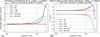 |
Figure 3. Calculation of (A) the acoustic impedance and (B) the volume transfer ratio of a rectangular slit (L s = 400 μm, h s = 30 μm) according to the LRF model, the FLNS finite-element model, and the simplified expressions for the Reynolds regime (s 2 ≪ 1). |
The calculation of the acoustic parameters of a curved cavity are shown in Figure 4. A mesh consisting of 30 elements across g0 and 50 divisions across L was configured for the finite-element model (simulating only one-half of the structure in the positive x-axis due to symmetry). The profiles of the distributed force calculated by the LRF method (case I) correspond nearly exactly to those obtained by the FLNS simulation. The assertion that only the zeroth and first propagation modes are relevant for the analysis of the cavity can be verified qualitatively: the profile of the distributed force resembles a cosine function shifted by a mean value. The calculation of the friction coefficient by LRF (case I) and FEM also yield the same results. Application of the approximation for a thin actuator (case II) resulted in a slight overestimation of the real part of the friction coefficient. A further simulation possibility was explored for this case, consisting of a two-dimensional finite-element model whose gap is fitted to approximate the friction coefficient of the full structure. Such a reduction from a three-dimensional to a two-dimensional geometry would only be meaningful for the case of negligible lateral flow, for which equation (74) was derived. The pressure profile calculated for this “effective slice” should correspond to the average value, when integrating across the beam’s length, so that the projected force can be calculated as Fb = wavgχL. Likewise, the velocity with which this slice is excited should correspond to the average velocity of the beam, so that the equivalent velocity at the midpoint can be calculated as vb = vavg/χ. Noticing that the ratio between distributed load and wall velocity for a two-dimensional slice in the Reynolds regime is given by equation (73), we can propose an expression for the effective gap (geff) of such a slice (Eq. (86)). Therefore, the question is whether the simulation of this equivalent two-dimensional structure, not with the Reynolds equations but with FLNS, results in approximately the same friction coefficient as the three-dimensional FLNS simulation. According to the results in Figure 4B, the effective gap approximation is very close to the outcome of the three-dimensional model, but requiring a significantly lower computational cost. For designs where L ≫ h, this two-dimensional “effective gap” model is an interesting alternative for a quick validation. While the three-dimensional model requires tens of minutes of computation time, the two-dimensional model may just require a few minutes and the analytic model merely the fraction of a second – hence the benefit of approximate models.
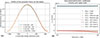 |
Figure 4. Calculation of (A) the distributed force and (B) the effective friction coefficient of a curved cavity (g 0 = 5 μm, s 0 = 1 μm, a 0 = 1 μm, h = 75 μm, L = 900 μm) according to the LRF model, the FLNS finite-element model, and the approximate two-dimensional model with an “effective gap”. |
 (79)
(79)
![Mathematical equation: $$ \begin{aligned} \rightarrow g_{\text{ eff}}&= g_0 \left[\frac{2\chi ^2}{\mathrm{\Theta }(z_{\rm DC}-\sigma _s)}\right]^{1/3}. \end{aligned} $$](/articles/aacus/full_html/2026/01/aacus250087/aacus250087-eq164.gif) (80)
(80)
3.2 Simulation of the L-CMUT structure
The acoustic parameters of sample L-CMUT design, whose most relevant dimensions are listed in Table 1, were simulated according to the approximate analytical model and through finite-element models. The three-dimensional model of the structure (covering only the half of the structure in the positive x-axis due to symmetry) captures the variation of the boundaries that correspond to the deflected shape of the beam in its biased state3. The velocity at each point of this boundary is also modulated in the x-axis according to the ϕ0 function. Some nodal plots of this model are shown in Figures 5A and 5B. On the other hand, the two-dimensional model of this device consists of only one element in the x-axis, and its electrostatic gap was adjusted to the effective value proposed in equation (86). In both cases, a slight correction for the viscosity in the the 1 μm clearance was performed, following the model from Veijola et al. [11], due to the potentially high Knudsen number in this section. They propose to adjust the viscosity with the Knudsen number according to μ′=μ/(1 + 9.638(Kn)1.159), which reduces its value by 30% (Kn ≈ 0.06). If the same correction is applied to the ∼5 μm electrostatic gap, the correction would be around 6%; therefore, until a model is developed for slip flow in a non-uniform structure, this small adjustment will be neglected for the case of the cavity.
Dimensions of an L-CMUT design.
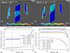 |
Figure 5. Acoustic simulation of the complete L-CMUT structure. Nodal plots obtained by the three-dimensional FEM: (A) pressure and (B) particle velocity in z (“y” axis in the ANSYS code). Comparison of (C) the equivalent friction coefficient, ceq, and (D) the equivalent piston area, Seq, according to the simplified analytical model, the two-dimensional FEM, and the three-dimensional FEM. |
A comparison of the outcome of the three models can be appreciated in 5C and 5D. The analytic model estimates the friction coefficient (ceq) rather well, save for an overestimation of its increment at high frequencies. A slight discrepancy can also be observed between the three-dimensional and two-dimensional FEMs, which could indicate a moderate contribution of lateral flow. The effective piston area (Seq) is overestimated by the analytical model by a factor of ∼1.25, so a surplus of ∼2 dB in the sound pressure level is expected to be predicted by this simplified model. A correction of the effective piston area would require a careful consideration of the coupling between slit and cavity; nonetheless, this model appears to be good enough for a first estimation of the performance in the design phase. The two- and three-dimensional models barely differ from one another in the calculation of this parameter.
4 Comparison against experiments
A sample L-CMUT chip was placed in front of a calibrated microphone (GRAS ®46DP-1) at a distance of 15 cm with the aid of a motorised linear stage (PI®M-403.8DG), within an anechoic chamber, as depicted in Figure 6A. A flat structure, 10 × 8 cm2, surrounds the L-CMUT in order to replicate the effect of a baffled radiation (albeit certainly not an “infinite baffle”). A burst of 10 periods at the frequency of interest, modulated by a Hann window, was generated with an oscilloscope (Rohde & Schwarz ®RTB200). The signal amplitude was increased to 10 V (peak) and superimposed to a 30 V bias voltage with a Krohn–Hite ®7600M amplifier. This measurement strategy proved effective to suppress reflections, which would otherwise be present in a continuous measurement.
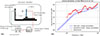 |
Figure 6. (A) Scheme of the measurement loop used to determine the radiated sound pressure level (SPL) from a fabricated L-CMUT. (B) Comparison of the measured SPL against the two-dimensional finite-element model and the approximate analytical model. |
A comparison of the radiated sound pressure level (SPL), both as measured and as simulated by the analytic model and the two-dimensional FEM, is presented in Figure 6B. The complex-valued, frequency-dependent effective piston area (S e q ) and friction coefficient (c e q ) of both models were incorporated to the same network model of the electromechanical interactions – see [1, 3] for more details. The radiation characteristic of the 10 × 8 cm2 baffle was calculated in a separate simulation and incorporated into the model as well. The outcome of the analytical model is indeed about 2 dB higher than that of the finite-element simulation, as predicted, and follows the same trend with frequency. These models come close to the experimental results, although not exactly. There are frequencies in which the measured curve intersects the simulated curves, but some features remain to be predicted by the theory. It is important to note that the prediction of the SPL is the final outcome of three modelling stages: the electromechanical network, the visco-thermal model, and the radiation pattern. Although the first two have been the subject of intense research, the third one is in an early stage of development. One reason to attribute the observed deviations to the simulated radiation pattern is because small errors in the actual dimensions of the microbeam and the microchanels (or in the assumed properties of the involved solids and gases) would lead to a shift of the theoretical curve, whether vertically or horizontally, but not to the unexpected hills and valleys that the experimental curve exhibits. Furthermore, the exact description of the immediate surroundings of the chip has a significant impact on the radation characteristics. Nonetheless, the presented model serves as a feasible first estimation of the behaviour of an L-CMUT as a transmitter.
5 Conclusion
By applying the Low Reduced Frequency (LRF) approximation to the Navier–Stokes equations in rectangular coordinates, the visco-thermal propagation of acoustic waves in a rectangular slit and in a cavity with curved boundaries could be solved analytically in two particular cases: small thickness variations and large width-to-depth aspect ratios. The solution of these equations within these application cases was found to be in good agreement with equivalent finite-element simulations that solve the Full Linearised Navier–Stokes equations. The analysis of these two components serves to formulate an approximate model of the microchannels in an in-plane electrostatic transducer (“L-CMUT”), whereby waves are losslessly transferred from the cavity to the slit despite the abrupt change in the cross section. The outcome of this model was compared against two- and three-dimensional finite-element models of the complete structure of the device. The approximate analytical model, although slightly overestimating the radiated sound pressure level, serves as a good first estimation of the acoustic performance of an L-CMUT design. If the ratio of the microbeam’s length to its width is large enough, a very accurate two-dimensional simulation with an “effective electrostatic gap” can be performed for the cavity (and hence also for the complete structure), enabling a rapid estimation of the acoustic parameters with little loss of precision. The results of these simulations were found to resemble the measured curves of the radiated SPL in an actual design, although there are features in the experimental curve that were not predicted by the theory and require a closer examination of the radiation pattern. The implementation of LRF proved suitable for the frequency range of interest but cannot be extended to frequencies near the MHz-range, where further visco-thermal effects gain prominence. The assumption of a lossless coupling between cavity and slit – being the simplest of methods to construct a model of the complete device – systematically overestimates the generated SPL by a slight amount in this case of free-field radiation, but in cases where the acoustic load is significantly higher a more careful coupling mechanism should be proposed. Overall, the gain of developing an analytic acoustic model lies, on the one hand, in the intuition that the designer earns with regard to the critical dimensions and the underlying mechanisms, and, on the other hand, in the reduced computation time compared to a finite-element simulation, especially if an optimisation or a parametric study needs to be performed.
Funding
This work was financed by the German Ministry of Education and Research (BMBF) in the project iCampμs Phase II (2111M194).
Conflicts of interest
The authors declare no conflict of interest.
Data availability statement
Data are available on request from the authors.
Author contribution statement
JMM and HAGS solved the analytical equations in parallel, verifying each other’s results. JMM programmed the numerical simulations and performed the experiments.
References
- J.M. Monsalve, A. Melnikov, M. Stolz, A. Mrosk, M. Jongmanns, F. Wall, S. Langa, I. Marica-Bercu, T. Brändel, M. Kircher, H.A. Schenk, B. Kaiser, H. Schenk: Proof of concept of an air-coupled electrostatic ultrasonic transducer based on lateral motion. Sensors and Actuators A: Physical 345 (2022) 113813. [Google Scholar]
- W.M. Beltman: Viscothermal wave propagation including acusto-elastic interaction. Dissertation, University of Twente, 1998. [Google Scholar]
- H.A.G. Schenk, A. Melnikov, F. Wall, M. Gaudet, M. Stolz, D. Schuffenhauer, B. Kaiser: Electrically actuated microbeams: an explicit calculation of the Coulomb integral in the entire stable and unstable regimes using a Chebyshev–Edgeworth approach. Physical Review Applied 18 (2022) 014059. [Google Scholar]
- M.R. Stinson: The propagation of plane sound waves in narrow and wide circular tubes, and generalization to uniform tubes of arbitrary cross-sectional shape. Journal of the Acoustical Society of America, 89, 2 (1990) 550–558. [Google Scholar]
- M. Reed, B. Simon: Functional Analysis, in: Methods of Modern Mathematical Physics, Vol. 1. Academic Press, Cambridge, 1980. [Google Scholar]
- L.N. Trefethen, M. Embree: Spectra and Peudospectra: The behaviour of Nonnomal Matrices and Operators. Princeton University Press, Princeton and Oxford, 2005. [Google Scholar]
- L.L. Beranek, Acoustics. Acoustical Society of America, 1954. [Google Scholar]
- A. Melnikov, H.A.G. Schenk, F. Wall, J.M. Monsalve, L. Ehrig, M. Stolz, A. Mrosk, S. Langa, B. Kaiser: Squeeze film damping by a structured cavity inan air-coupled electrostatic ultrasonic transducer, in: Proc. SPIE 11955, Microfluidics, BioMEMS, and Medical Microsystems XX, Vol. 1195504, 2022. [Google Scholar]
- F. Wall, H.A.G. Schenk, A. Melnikov, J.M. Monsalve: Squeeze film damping by a structured cavity in an air-coupled electrostatic ultrasonic transducer. Proceedings of the 29th International Congress on Sound and Vibration ICSV29, No. 210, 2023. [Google Scholar]
- A. Sommerfeld: Lectures on Theoretical Physics. Academic Press, New York, 1954, pp. 361–373. [Google Scholar]
- T. Veijola, H. Kuisma, J. Lahdenperä, T. Ryhänen: Equivalent-circuit model of the squeezed gas film in a silicon accelerometer. Sensors and Actuators A: Physical 48, 3 (1995) 239–248. [Google Scholar]
Capacitive Micromachined Ultrasound Transducer.
These quantities are complex numbers. We use the convention j for the imaginary unit (j2 = −1).
Capacitive transducers need to be biased with a dc voltage, around which they oscillate upon excitation.
Cite this article as: Monsalve J.M. & Schenk H.A.G. 2026. A visco-thermal model for a novel type of electrostatic micromachined in-plane ultrasound transducer. Acta Acustica, 10, 8. https://doi.org/10.1051/aacus/2026004.
All Tables
All Figures
|
Figure 1. (A) Photograph of a fabricated L-CMUT and scheme of (B) its top view and (C) its cross section. The device consists of a beam that is pulled towards a stator by an electrostatic force. As this occurs, the gas in the cavity between beam and stator is expelled towards the slits and then departs from the chip, emitting ultrasound waves. |
| In the text | |
|
Figure 2. Illustration of the dimensions and coordinates used to describe the geometry of the slits and the beam-stator cavity of an L-CMUT. |
| In the text | |
|
Figure 3. Calculation of (A) the acoustic impedance and (B) the volume transfer ratio of a rectangular slit (L s = 400 μm, h s = 30 μm) according to the LRF model, the FLNS finite-element model, and the simplified expressions for the Reynolds regime (s 2 ≪ 1). |
| In the text | |
|
Figure 4. Calculation of (A) the distributed force and (B) the effective friction coefficient of a curved cavity (g 0 = 5 μm, s 0 = 1 μm, a 0 = 1 μm, h = 75 μm, L = 900 μm) according to the LRF model, the FLNS finite-element model, and the approximate two-dimensional model with an “effective gap”. |
| In the text | |
|
Figure 5. Acoustic simulation of the complete L-CMUT structure. Nodal plots obtained by the three-dimensional FEM: (A) pressure and (B) particle velocity in z (“y” axis in the ANSYS code). Comparison of (C) the equivalent friction coefficient, ceq, and (D) the equivalent piston area, Seq, according to the simplified analytical model, the two-dimensional FEM, and the three-dimensional FEM. |
| In the text | |
|
Figure 6. (A) Scheme of the measurement loop used to determine the radiated sound pressure level (SPL) from a fabricated L-CMUT. (B) Comparison of the measured SPL against the two-dimensional finite-element model and the approximate analytical model. |
| In the text | |
Current usage metrics show cumulative count of Article Views (full-text article views including HTML views, PDF and ePub downloads, according to the available data) and Abstracts Views on Vision4Press platform.
Data correspond to usage on the plateform after 2015. The current usage metrics is available 48-96 hours after online publication and is updated daily on week days.
Initial download of the metrics may take a while.