| Issue |
Acta Acust.
Volume 10, 2026
|
|
|---|---|---|
| Article Number | 20 | |
| Number of page(s) | 13 | |
| Section | Environmental Noise | |
| DOI | https://doi.org/10.1051/aacus/2026016 | |
| Published online | 03 April 2026 | |
Scientific Article
Heat pump noise: Determination and modelling of preference-equivalent levels
Institute for Hearing Technology and Acoustics, RWTH Aachen University, 52074 Aachen, Germany
* Corresponding author: This email address is being protected from spambots. You need JavaScript enabled to view it.
Received:
25
July
2025
Accepted:
11
February
2026
Abstract
Air-to-water heat pumps are increasingly replacing traditional heating systems because of their environmental and energy benefits. However, noise emitted by their fans and compressors can cause complaints, even when regulatory limits are met. In this study, two listening experiments were conducted to examine heat pump noise by quantifying it as level penalties for equivalent loudness and preference. The study investigates how the preference-equivalent level differs from the loudness-equivalent level compared to a reference stimulus, and which psychoacoustic parameters best model the resulting level adjustments. Recordings from two heat pumps were auralised into a suburban residential setting and adjusted to an initial level of 60 dB(A). A two-alternative forced-choice (2-AFC) method with a 1-up-1-down rule is used to determine the point of subjective equality (PSE) for loudness and preference. Statistical analyses show significant differences between loudness-equivalent and preference-equivalent levels for eight of twelve stimuli. The median values further indicate that achieving equal preference relative to the reference generally requires lower sound pressure levels than achieving equal loudness, with the magnitude of this level offset varying across stimuli. Combining the results with psychoacoustic parameter analyses, two models based on linear regression were developed. This linear approach was chosen to ensure straightforward interpretability and robustness for the given stimulus set. Perceived loudness can be modelled by the psychoacoustic parameter loudness, while preference is best modelled by a linear combination of sharpness and roughness. These findings emphasise the need for perceptual metrics beyond A-weighted sound pressure levels when evaluating and optimising heat pump noise.
Key words: Heat pump noise / Psychoacoustic modelling / Loudness / Preference / Level penalty
© The Author(s), Published by EDP Sciences, 2026
 This is an Open Access article distributed under the terms of the Creative Commons Attribution License (https://creativecommons.org/licenses/by/4.0), which permits unrestricted use, distribution, and reproduction in any medium, provided the original work is properly cited.
1 Introduction
In 2023, 356 000 heat pumps were sold in Germany, 90% of which are air-to-water heat pumps [1]. The acoustic characteristics of air-to-water heat pumps can have an influence on their acceptance and, therefore, on the widespread use of this technology. The fan(s) and compressor are the dominant sources of noise [2]. However, the sound immission, i.e. the sound pressure level and its acoustic characteristics at the receiver, depends on the installation situation of the components, the installation location of the heat pump, and its operating state.
In a comprehensive review of air-to-water heat pump noise in residential settings, Langerova et al. [3] criticised current evaluation practices for primarily relying on single-value metrics such as the A-weighted sound power level. They emphasised the importance of detailed spectral analyses and standardised testing procedures to adequately assess tonal and low-frequency components. Furthermore, when considering the operation of air-to-water heat pumps with regard to high-efficiency and low-noise emissions, there is a conflict between energy-efficient operating states and operating states with reduced noise emissions [4]. However, within the IEA HPT Annex 51 Task 4 [2], Vering et al. [4] demonstrated that a simultaneous optimisation of both energy efficiency and acoustic performance is possible. Building on this approach, Schmidt and Müller [5] developed an acoustically improved heat pump demonstrator by selecting low-noise components and focusing on the reduction of sound emissions under realistic operating conditions.
Several studies have examined heat pump noise and explored how psychoacoustic parameters can be used to describe or model its perceptual impact. Kasess et al. [6] conducted an annoyance rating study on heat pump noise and investigated direction dependency. They found a strong effect of direction on the rated annoyance, which could be explained by the directivity of the noise of their heat pump. Yet, they noted that this pronounced direction dependence was likely due to the proximity of the microphones to the heat pump. Consequently, the overall annoyance of the heat pump was not assessed, as the measurements were limited in their distance from the heat pump. In addition to the directional analysis, Kasess et al. evaluated how well acoustical and psychoacoustical parameters could explain the annoyance ratings. Their regression analysis showed that A-weighted level and loudness accounted for most of the variance, while the inclusion of sharpness and roughness increased the explained variance only to a smaller degree. Acun et al. [7] conducted a listening experiment to assess human responses to air-source heat pump noise under different operating conditions, source distances, and background noise levels. Their analysis examined how subjective responses varied with operating cycles, audibility over background noise, and changes in psychoacoustic parameters. Across all conditions, annoyance was positively correlated with loudness, tonality, and roughness, while sharpness showed a weak negative correlation. Feldmann [8] conducted listening experiments to investigate the sound quality of ventilation units and heat pumps, applying psychometric methods such as semantic differentials, rating scales, and paired comparisons. Her results showed that loudness, tonality, roughness, and sharpness significantly influence the subjective evaluations that form the basis for her sound quality model. Nevertheless, her analysis focused solely on the fan component, excluding other relevant sound sources of the heat pump unit.
Instead of applying a rating-scale method, as is commonly done in similar studies, the present work employs the Point of Subjective Equality (PSE) method. Originating from classical psychophysics [9], the PSE aims to determine the point at which a stimulus on a physical scale is psychologically equivalent to another stimulus on the same scale by taking one of the stimuli as the reference. It yields a physically interpretable measure that is sensitive to even small perceptual deviations. By using sound pressure level as the varying parameter, the resulting PSE values can be interpreted as equivalent level penalties in decibels (dB) assigned to stimuli based on their sound characteristics. The PSE method is particularly suitable for evaluating heat pump noise because it provides precise, level-based perceptual equivalences and avoids biases inherent to rating-scale methods.
Töpken et al. [10] conducted a study using the PSE method in which they determined loudness and preference judgements of multi-tone sounds. They showed that a decrease in level reduces not only the perceived loudness but also the preference of a multi-tone sound. Furthermore, it was shown that additional level reductions were necessary to get from equal loudness to equal preference. Töpken and van de Par [11] used the PSE method further to build a model for predicting the preference-equivalent level for fan noise. Claaßen et al. [12] expanded upon the existing research by exploring different reference sound pressure levels to refine the models for fan noise. The best models from both studies are based on spectral weighted specific loudness parameters, which were introduced by Töpken and van de Par [13]. Models based on sharpness were also investigated, but they have not proven to be as successful. Other established psychoacoustic parameters, like tonality or roughness, were not considered as model parameters. Töpken and van de Par [13] also showed that fan noise can be categorised into distinct groups even when they are presented at the same sound pressure level.
Yet, rather than focusing solely on fan noise, the research presented here investigates the comprehensive sound profile of heat pump units. This broader focus is essential because fan-only approaches can not capture the perceptual impact of the full acoustic emission. This enables examining whether, and to what extent, the findings align with those reported for fan noise.
Previous studies either recorded sound stimuli in climate chambers [6] or did not specify the recording method. Alternatively, field measurements of operating heat pumps are performed in residential areas, such as in the work by Sangsinsorn and Nienborg [14]. They highlighted the importance of considering realistic environmental conditions when evaluating the acoustic impact of heat pumps. Therefore, the investigated sounds in this study were recorded from air-to-water heat pumps in a hemi-anechoic chamber and afterwards auralised. Auralisation refers to the generation of an audible representation of an acoustic scenario based on simulated sound propagation and signal processing [15]. This approach provides stimuli that incorporate realistic propagation effects while maintaining full experimental control, thereby enabling ecologically relevant yet reproducible listening conditions.
The study presented in this paper investigates the perceptual evaluation of air-to-water heat pump noise using binaural auralisations of measured recordings embedded in a realistic suburban backyard scenario. Two listening experiments were conducted to examine how adjustments in sound pressure level influence perceived loudness and preference relative to a reference stimulus. To ensure that the evaluation in the listening experiments of the study presented in this paper was not influenced by initial level differences between the heat pump stimuli, they were first adjusted to the same A-weighted sound pressure level. During the listening experiments, the level of the stimuli was then adaptively varied to find the PSEs for loudness and preference, following the method used in previously mentioned studies [10–12]. To allow comparison with previous studies, preference can be considered to be negatively linked to short-term annoyance. Short-term annoyance refers to annoyance assessed in listening experiments and, following the recent discussion by Lotinga and Torija [16], should not be equated with long-term annoyance assessed in observational social survey settings. In addition to the perceptual data, psychoacoustic parameters were analysed to explore their potential for describing the observed loudness and preference judgements. The study is guided by two research questions:
-
How do the preference-equivalent levels differ from the loudness-equivalent levels across a diverse set of stimuli from heat pumps, and to what extent is this difference consistent or stimulus-dependent?
-
Which psychoacoustic parameters or combinations thereof best model the level adjustments derived from the PSEs for loudness and preference?
2 Method
2.1 Measurements
The outdoor units of two monobloc air-to-water heat pumps were installed in hemi-anechoic chambers. The first heat pump (Mitsubishi Electric PUZ-WM112YAA) was selected as a representative model commonly used in German single-family homes and available on the open market at the time of purchase. The second heat pump was developed as an acoustically improved air-to-water heat pump demonstrator [5]. The installation of the first heat pump took place at the Institute for Hearing Technology and Acoustics, RWTH Aachen University, Aachen, Germany, while the second was at Viessmann Holding International GmbH, Allendorf (Eder), Germany. For the first heat pump, additional details on the measurements are provided in a corresponding technical report [17]. In brief, the outdoor unit was installed in a hemi-anechoic chamber (V ≈ 300 m3, f g ≈ 100 Hz) and recorded using a 1/2′′ low-noise microphone (G.R.A.S. 40HL) positioned at a radial distance of 3 m from the centre of the heat pump in the direction of the front, with an angle of 30° to the frontal centre. The room temperature in the chamber varied between 3 °C and 11 °C during the measurement, allowing the heat pump to operate in different operating states, namely high-power heating, maximum capacity (winter mode), and defrost. In addition, the horizontal directivity of the heat pump was measured using 12 Sennheiser KE 4-211-2 microphones positioned in 30° steps around the device at a height of 0.58 m and a distance of 1.86 m from its centre, corresponding to the mid-height of the outdoor unit. The recordings and directivity measurements were conducted in a similar manner for the second heat pump at Viessmann Holding International GmbH, Allendorf (Eder), Germany.
2.2 Auralisation
Especially in psychoacoustic studies, where the focus is on the investigation of sound perception, auralisation is a tool for creating plausible acoustic scenarios in a controlled laboratory experiment [15]. To contextualise the anechoic recordings of the heat pumps in a realistic setting, sound propagation within a backyard scenario was simulated using the ray-based simulation software RAVEN [18, 19], which has been validated with respect to the sound propagation simulation in the scope of other projects in the past [20–22]. The propagation of the recorded heat pump noise was binaurally auralised, accounting for the directivity of the heat pump and the interaction of the sound with the surrounding environment. The directivitiy of the first heat pump were computed from the measured directivity data of the respective heat pump, which was processed from the multi-channel heat pump recordings [17], and is provided in the supplementary materials in openDAFF format. The 3D model of the scene, shown in Figure 1 left, represents a typical suburban residential setting. The heat pump, marked by the blue square, is positioned at the back of the neighbouring house in front of a wooden fence. The red dot indicates the receiver’s position on the terrace, facing the heat pump with a slight head rotation to the right, resulting in a more dominant sound incidence at the left ear. A top-view geometry specifies the source-receiver distance of 13.1 m with an additional lateral displacement of 0.4 m, cf. Figure 1 right. The environmental and material properties used for the sound-propagation simulation were as follows: a temperature of 20 °C, a relative humidity of 50%, an air pressure of 101 325 Pa, and mean absorption coefficients of α = 0.045 for concrete, α = 0.308 for grass, and α = 0.100 for the wooden fence. The used absorption and scattering data, along with plots, are available in the supplementary materials. The 3D model was developed using software SketchUp 2016 and is included as .skp files as well as in the open, ASCII-based .obj format.
 |
Figure 1. 3D model (left) and top view (right) of the scene used for the auralisation. The blue square marks the position of the source, the heat pump. The red dot marks the position of the receiver. The top-view geometry specifies the source-receiver distance of 13.1 m with an additional lateral displacement of 0.4 m. |
2.3 Stimuli
Six recordings from each heat pump were chosen to represent their operational range with respect to psychoacoustic metrics. The six stimuli of the first heat pump will be indicated by capital letters A through F. The mapping between stimuli and the corresponding recording numbers in [17] is as follows: A - 22, B - 25, C - 1, D - 9, E - 11, F - 13. The measured sound power levels of these recordings ranged between 60.4 and 69.0 dB(A), and the rotational frequency of the fan ranged from 495 to 753 rpm. All recordings except number 25 (later referred to as stimulus B) represent the operating state high-power heating, whereas recording 25 corresponds to maximum capacity, which is reflected in its increased sound power level and rotational frequency. The signals of the second heat pump, recorded at Viessmann Holding International GmbH, will be indicated by lowercase letters a through f. Matching letters between the two datasets does not indicate a correspondence in psychoacoustics or operating states between them. All stimuli represent real-world operating states of the respective heat pump. Fan and compressor sounds were not recorded separately. The heat pumps were treated as single acoustic sources, and the recordings capture their complete operational noise as it occurred naturally. Consequently, the recordings may contain additional housing-related sounds (e.g., light rattling), which are not separately controllable. Different operating states characterise the audible differences between the stimuli. The sound pressure levels of the recorded heat pump stimuli A to F are between 42.8 and 53.2 dB(A), and of the stimuli a to f between 28.3 and 38.7 dB(A), measured at a distance of 3 m. To establish comparable conditions across stimuli, they were set to an initial sound pressure level of 60 dB(A). This level was selected to ensure that all characteristic features and perceptual differences between the heat pump stimuli were clearly audible. The heat pump stimuli A to F, set at an equal level of 60 dB(A), are available in the supplementary material. Each heat pump stimulus, also referred to as test stimulus in the following, was compared to a reference stimulus. This reference stimulus was generated by filtering white noise to approximate the specific loudness of the measurement recordings from stimuli A to F, acknowledging that an exact match was not achievable. Figure 2 left shows the specific loudness as a function of critical band rate for the reference stimulus and the measurement recordings, prior to auralisation and the equalisation. The right panels depict the specific loudness of the stimuli as prepared for the listening experiments, after auralisation and equalisation to 60 dB(A). The top panel shows the stimuli from the first heat pump (A–F) compared to the reference stimulus, which was fixed at 60 dB(A) during the listening experiments. Similarly, the bottom panel displays the stimuli from the second heat pump (a–f) alongside the reference stimulus. The reference stimulus is also given as supplementary material, both before and after the auralisation.
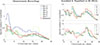 |
Figure 2. Specific loudness N′ as a function of critical band rate z: The left plot shows the measurement recordings A to F along with the reference stimulus, while the right plot depicts the stimuli used in the listening experiments after being auralised and equalised to 60 dB(A). The top panel on the right displays the stimuli from the first heat pump (A–F), whereas the bottom panel shows the stimuli from the second heat pump (a–f), each compared with the auralised reference, also at 60 dB(A). Depicted are the values for the left ear. |
2.4 Listening experiments
Two independent listening experiments were conducted, spaced six months apart. The first experiment included stimuli labelled A to F, while the second used stimuli labelled a to f, lowercase letters. These experiments aimed to quantify differences in perceived loudness and preference as equivalent sound pressure levels using an adaptive measurement method to determine the PSE. The methodology is a 2-AFC with a 1-up-1-down rule. A sketch of the procedure can be seen in Figure 3. The underlying assumption is that a decreasing level reduces the perceived loudness and increase the preference of a sound.
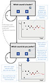 |
Figure 3. Sketch of the procedure for the listening experiments. For each test stimulus, the 2-AFC method is combined with a 1-up-1-down rule. |
Prior to the experiment, participants were informed that the sounds originated from an air-to-water heat pump, but no additional contextual information about the simulated environment was provided. In each trial, the participants listened to one of the test stimuli and the reference stimulus, and were asked either to select the louder stimulus or the one they preferred by answering the question Which sound is louder? or Which sound do you prefer?. Each stimulus lasted 3.5 s, with a 0.5 s pause between the two stimuli. The stimuli could be replayed within a trial without limitation. In both listening experiments, half of the participants began with the loudness question, while the other half started with the preference question. Each participant completed all test stimuli for one question type before proceeding to the other. The sequence of presenting the test stimulus first or second was randomised for each trial, and the overall order of stimuli was counterbalanced across participants. At the start of the listening experiment, the test stimuli and the reference stimulus were set to a sound pressure level of 60 dB(A). While the reference stimulus consistently remained at 60 dB(A), the sound pressure level of the test stimulus varied, increasing or decreasing based on the response of the participant to the question asked. If the participant changed their loudness or preference judgement (e.g., they initially perceived the test stimulus as louder but then judged the reference stimulus as louder after adaptation), this marked a reversal point in the adaptive track. After each upper reversal point, the step size of the level adjustment was halved, starting from 6 dB to 3 dB, continuing until a minimum step size of 1.5 dB was reached. Each stimulus block concluded after eight reversal points, and the next block began with the next test stimulus. The resulting (PSE) level was calculated as the mean value of the last four reversal points. This level, at which the test stimulus is perceived as equally loud Lloud or as equally preferred Lpref as the reference stimulus, is referred to as the PSE. If a participant required more than 25 trials, the block ended, and the listening experiment proceeded with the next test stimulus. The block also concluded if the test stimulus level dropped below 30 dB(A) or exceeded 80 dB(A). The experiments were implemented in MATLAB App Designer and conducted in one of the listening booths at the Institute for Hearing Technology and Acoustics, RWTH Aachen University, Aachen, Germany. The stimuli were calibrated by measuring the sound pressure level at the ear canal entrance of the ITA Artificial Head [23] using the ITA toolbox in MATLAB [24]. The stimuli were presented using Sennheiser HD 650 headphones and each experiment lasted an average of 50 min.
In the first listening experiment, data from one block of one participant in the loudness task and from three blocks of another participant in the preference task were excluded from the evaluation. One exclusion was due to a self-reported judging error, and the other occurred because the participant reached below the minimum level of 30 dB(A). Consequently, data from all 20 participants (12 female, 8 male) were included in the analysis, with the exception of the specific blocks mentioned above. All participants were confirmed as normal-hearing using audiometry and ranged in age from 20 to 34 years (mean: 25 years).
In the second listening experiment, data from two participants in the loudness task and from one participant in the preference task were not collected due to technical issues. Thus, data from all 24 participants (10 female, 14 male) were included in the analysis, excluding the missing data. All participants were confirmed as normal-hearing via audiometry and were aged between 22 and 34 years (mean: 25 years).
3 Results
3.1 Psychoacoustic parameters
Before looking at the results of the listening experiments, the evaluation of psychoacoustic parameters is presented. The values for loudness N, sharpness S, roughness R, and tonality T for the left ear, the dominant ear, of the twelve test stimuli and the reference stimulus were calculated using ArtemiS SUITE 13.1. The psychoacoustic parameters were calculated based on the initial stimuli, which were adjusted to an equal A-weighted sound pressure level of 60 dB(A), and are shown in Figure 4. The loudness N in sones was calculated using the standard ISO 532-1 [25] and is plotted on the top-left panel. Stimulus F has the lowest loudness at 12.1 sone, while the reference stimulus has the highest value at 15.2 sone. The top-right panel shows the sharpness S in acum, calculated according to DIN 45692 [26]. For stimuli A to E, the sharpness varies by a maximum of 0.08 acum and thus might be perceived as equally sharp, considering reported JND values of 0.08 acum [27]. Stimulus F exhibits the highest sharpness value at 1.81 acum. Stimuli a to c range from 1.49 to 1.54 acum, while the sharpness for stimuli d to f increases progressively, reaching up to 1.76 acum. The reference stimulus has a sharpness of 1.6 acum. The lower-left panel shows the roughness R in asper, calculated according to ECMA-418-2 (1st edition) [28]. The values range from 0.03 to 0.31 asper, with the reference stimulus having the lowest roughness. According to ECMA-418-2 (1st edition) [28], the perceptual threshold for prominent roughness is approximately 0.2 asper. Therefore, it is likely that only stimuli A, E, e, and f would be perceived as slightly (if at all) rough. Tonality T also varies substantially between the stimuli, as shown in the lower-right panel. It was calculated according to ECMA-74 (17th edition) [29] and ECMA-418-2 (1st edition) [28]. Stimulus B exhibits the lowest tonality at 0.11 tuHMS, while stimulus f has the highest value at 0.73 tuHMS. It is worth noting that even for the reference stimulus, which is filtered white noise and in principle neither rough nor tonal, the roughness and tonality values are greater than zero. The spectrally weighted specific loudness parameters Nlow and Nratio, introduced by Töpken and van de Par [13] for PSE prediction of fan noise, were also calculated. Nlow represents the ratio of specific loudness from 0 to 2.5 Bark relative to the total loudness N of the stimulus, while Nratio reflects the ratio of specific loudness in the range from 2 to 5 Bark to that in the range from 10 to 24 Bark. However, these parameters did not provide meaningful differentiation due to rather small variations among the stimuli. The observed ranges were 0.32 to 0.56 for Nratio and 0.05 and 0.11 for Nlow.
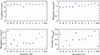 |
Figure 4. Values of the psychoacoustic parameters loudness in sone, sharpness in acum, roughness in asper, and tonality in tuHMS for the twelve test stimuli (stimuli A–F of the first experiment in blue circles, and stimuli a–f of the second experiment in violet squares) and the reference stimulus (red triangle). Depicted are the values for the left ear. The values are calculated for the initial sound pressure level of 60 dB(A). |
3.2 Point of subjective equality
The resulting PSEs for loudness Lloud and preference Lpref for all test stimuli can be seen in the left part of Figure 5. The median values and interquartile ranges across all participants are given. The dashed horizontal line indicates the fixed level of the reference stimulus at 60 dB(A). Examining the median values, increasing the level was necessary for nearly all stimuli to achieve equal loudness, while for equal preference, the level was decreased for eight of the twelve test stimuli by the participants. The interquartile ranges are smaller for the loudness PSEs than for the preference PSEs. For the statistical analysis, linear mixed-effects models were used to account for repeated measurements within participants and occasional missing observations. To quantify the differences between Lloud and Lpref within a stimulus, a linear mixed-effects model with Task, Stimulus, and their interaction as fixed effects with a random intercept for Participant was fitted across all observations. As twelve stimulus-specific tests were performed, p-values were adjusted for multiple comparisons using the Holm procedure. Significant differences (Holm-corrected p < 0.05) between Lloud and Lpref were found for stimuli A, B, C, E, F, d, e, and f, whereas no significant task differences were observed for stimuli D, a, b, and c. To assess whether the stimuli differed overall, linear mixed-effects models were fitted separately for the loudness and preference tasks. The models revealed significant main effects of Stimulus for both loudness (F(11, 182.04)=10.56, p < 10−14) and preference (F(11, 182.82)=9.04, p < 10−12), showing overall differences in PSE levels across stimuli. Post-hoc pairwise comparisons between stimuli were conducted as linear contrasts of the fitted mixed-effects model, and p-values were adjusted for multiple comparisons using the Holm procedure. For loudness, significant pairwise differences (Holm-corrected p < 0.05) were observed for stimulus F with all stimuli except B and c. Further for stimulus B with E, d, e, and f, as well as for e with c, and for f with A, C, D, a, b, and c. For preference, significant pairwise differences (Holm-corrected p < 0.05) were observed for stimuli B and D with f, and for stimuli a, b, and c with stimuli d, e, and f. Although significant effects were observed only for a subset of pairwise comparisons, the full set of descriptive median PSE values across all stimuli was retained for subsequent analyses. The relationship between Δ Lpref and Δ Lloud can be seen in the right part of Figure 5. Δ Lloud is the median relative level adjustment of the test stimulus required to be perceived as equally loud as the 60 dB(A) reference stimulus. Δ Lpref refers to the median relative level adjustment required for the test stimulus to be perceived as equally preferred as the reference stimulus. They are calculated by subtracting the level of the reference stimulus from the PSEs.
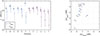 |
Figure 5. Left: median levels for equal loudness Lloud (filled) and equal preference Lpref (open) with interquartiles as errorbars for each stimulus across participants. The reference level of 60 dB(A) is indicated as dashed horizontal line. Right: relationship between the median level adjustment for equal preference Δ Lpref and the median level adjustment for equal loudness Δ Lloud. |
The median values for each stimulus across all participants are shown. Positive values indicate that the level of the test stimulus had to be increased to be perceived as equally loud or equally preferred compared to the reference stimulus. Conversely, negative values indicate that the level of the test stimulus had to be decreased to be perceived as equally loud or equally preferred compared to the reference stimulus. Δ Lloud is positive for all stimuli, except two (e and f), but Δ Lpref is only positive for four stimuli (B, D, b, and c). The stimuli F and f have the biggest difference between Δ Lloud and Δ Lpref with 6.8 and 7.0 dB. The smallest difference between Δ Lloud and Δ Lpref can be found for stimuli b and D with 0.6 dB. The level adjustments to reach equal loudness are between −0.6 and 3.7 dB, and for equal preference, they are between −7.5 and 1.1 dB. For all stimuli, Δ Lpref is lower than Δ Lloud. Regarding research question 1, the statistical analyses indicate that, for eight of twelve stimuli, the loudness-equivalent levels differ significantly from the preference-equivalent levels. Considering the median values, the preference-equivalent levels are consistently lower than the loudness-equivalent levels across all stimuli. Between-stimulus comparison reveal significant differences for only a subset. In particular, stimulus F, characterised by a high Lloud, and stimulus f, characterised by a low Lpref, differ significantly from most of the other stimuli.
When evaluating the loudness differences between the test stimuli and the reference stimulus before (ΔNinit) and after (ΔNresult, loud) the PSE Lloud determination (see Tab. 1), it becomes evident that the initial loudness differences are greater than or equal to the loudness JND (0.8 sone [30]). At their resulting levels, the loudness differences ΔNresult, loud fall within or below the JND threshold for most stimuli, except for stimuli e and f. These two stimuli were the only ones rated as louder than the reference stimulus in the experiment (indicated by a negative Δ Lloud), resulting in an even greater loudness difference. In Table 1, the Δ Nresult, pref, the loudness difference after the PSE Lpref determination, shows that the value is smaller or equal to Δ Ninit for only five stimuli. For all stimuli Δ Nresult, pref exceeds Δ Nresult, loud. Only stimuli D and b were rated similarly within the JND range. The substantial deviations from 0.5 up to 6.8 sone indicate that there are additional factors influencing the preference besides the psychoacoustic loudness. This descriptive pattern provides first indications related to research question 2, as the level adjustments required to reach equal loudness correspond well to the underlying loudness differences, whereas the level adjustments required to reach equal preference do not show such a correspondence.
The loudness difference between the initial loudness of the test stimuli subtracted from the loudness of the reference stimulus is labelled as Δ Ninit. Δ Nresult, loud and Δ Nresult, pref represent the differences between the loudness of the PSE levels, Lloud and Lpref, and the loudness of the reference stimulus.
Linear regression models and their statistical evaluation based on the psychoacoustic parameter loudness N for the level adjustment Δ Lloud and the level adjustment Δ Lpref. Given are R2, F-test and p-value of the linear regression.
4 Model
To examine whether the level penalties derived from the listening experiments can be described by psychoacoustic parameters, linear and multiple linear regression analyses were conducted. Linear regression was chosen due to its straightforward interpretability and its suitability for small datasets, such as the limited number of test stimuli in this study. This approach allows for a direct evaluation of how individual or combined psychoacoustic parameters relate to the level adjustments of loudness and preference. The loudness N, calculated in sone, effectively captures the perceived loudness difference, which was measured in the experiments as the PSE level Lloud. A linear regression showing the relationship between Δ Lloud and the psychoacoustic parameter loudness N is depicted with the grey dashed line in Figure 6. The negative slope of the linear regression shows that lower initial loudness values resulted in higher positive level adjustments for the loudness PSEs. The statistical analysis shows that this linear regression is significant (p < 0.05), compare the first row in Table 2, and therefore Δ Lloud can be represented by the psychoacoustic parameter loudness. The preference judgements Δ Lpref can not be explained by the psychoacoustic parameter loudness N using linear regression, as indicated by the statistics in the second row of Table 2. With an R2 value of 0.002 and a p-value of 0.88, loudness is not a suitable parameter for modelling Δ Lpref. Therefore, it is worthwhile to examine whether other psychoacoustic parameters better account for the observed data.
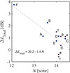 |
Figure 6. The level adjustment for equal loudness Δ Lloud in dB plotted against loudness N in sone. The linear regression fit is shown with the grey dashed line. |
Sharpness, tonality, and roughness show promising results for modelling the preference PSE. Δ Lpref is plotted against sharpness S (Fig. 7), tonality T (Fig. 8), and roughness R (Fig. 9). Linear regressions were performed for each psychoacoustic parameter, and the resulting regression lines are shown in the figures as grey dashed lines. For all three psychoacoustic parameters, the relationship to the level adjustments required to reach equal preference Δ Lpref is negative. Stimuli with higher sharpness, tonality, and roughness values needed to be reduced more in level to be perceived as equally preferred as the reference stimulus, resulting in negative Δ Lpref values. Conversely, stimuli with low sharpness, tonality, and roughness values required less level reduction, or in some cases even a level increase, to be perceived as equally preferred as the reference stimulus. The statistical outcomes of these regressions are summarised in Table 3, with the first three rows presenting the results for the individual parameters. The regressions for sharpness and tonality are both statistically significant (p < 0.05), while the regression for roughness is not statistically significant (p > 0.05). The last three rows of Table 3 present the results of multiple linear regressions combining the following psychoacoustic parameter pairs: sharpness and tonality, tonality and roughness, sharpness and roughness. Multiple linear regression was employed to assess whether combinations of psychoacoustic parameters provide a more accurate explanation of the preference judgements compared to individual predictors. All three models are statistically significant (p < 0.05). With the model combining sharpness and roughness yielding the best fit, with an R2 of 0.8 and a p-value of below 0.001. Figure 10 shows a 3D-plot of the relationships between Δ Lpref, sharpness S and roughness R. The more negative the Δ Lpref values, the higher the sharpness and roughness values, indicating that stimuli with high sharpness and roughness values were less preferred at their initial level compared to the reference stimulus. Stimuli with lower sharpness and roughness values resulted in positive Δ Lpref values, indicating that they were more preferred than the reference stimulus at the initial level before the adaptive adjustment.
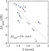 |
Figure 7. The level adjustment for equal preference Δ Lpref in dB plotted against sharpness S in acum. The linear regression fit is shown with the grey dashed line. |
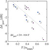 |
Figure 8. The level adjustment for equal preference Δ Lpref in dB plotted against tonality T in tuHMS. The linear regression fit is shown with the grey dashed line. |
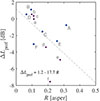 |
Figure 9. The level adjustment for equal preference Δ Lpref in dB plotted against roughness R in asper. The linear regression fit is shown with the grey dashed line. |
Statistic evaluation of six different (multiple) linear regression models based on the psychoacoustic parameters sharpness, tonality and roughness for the preference-equivalent level Δ Lpref. Given are R2, F-test and p-value of the linear regression.
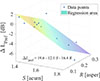 |
Figure 10. The level adjustment for equal preference Δ Lpref in dB plotted against sharpness S in acum and roughness R in asper. |
5 Discussion
The results of this study reveal that heat pump noises with an equal A-weighted sound pressure level are not perceived to be equally loud or equally preferred. This finding aligns with the results of the study by Töpken and van de Par [11], who similarly investigated fan noise. The applied experimental approach of adjusting the sound pressure level allows for identifying even small perceptual differences and is therefore often considered superior to direct scaling methods. Although the stimuli originated from just two heat pumps, variations in their operating led to distinguishable perceptual impressions, indicating that even changes within the same device can affect perception, particularly when assessed relative to a reference. Despite all stimuli being initially presented at the same A-weighted sound pressure level, the evaluated data from the listening experiments reveal that loudness and preference judgements for heat pump noise can differ noticeably. This shows that the A-weighted level by itself does not comprehensively account for perceptual differences. This critique aligns with Langerova et al. [3], who questioned the validity of A-weighted metrics for characterising the acoustic impact of heat pumps and called for more differentiated evaluation approaches. The change in sound pressure level required to achieve equal preference differs systematically from that required to achieve equal loudness: across all stimuli, the median of the preference-equivalent level Lpref lies below the median of the loudness-equivalent level Lloud, and only for two stimuli, the difference between Lloud and Lpref is close to the level JND for broad-band noise (0.5 dB [31]). This aligns with the general observation that perceptual characteristics such as tonality, sharpness, and roughness can influence preference beyond what loudness-based metrics alone capture (see e.g. [32, 33]). Further support for this descriptive pattern is provided by model-based stimulus-specific task contrasts, which were significant for eight out of twelve stimuli.
Claaßen et al. [12] reported at 60 dB(A) reference level that for unpleasant fan noise Lpref is about 4 dB lower than Lloud, while for pleasant fan noise the difference was negligible. In our data, stimuli F, e, and f show greater differences, up to 7 dB. In contrast, stimuli B, D, a, b, and c show differences between Lloud and Lpref of only 0.6 or 1.1 dB. When considering the psychoacoustic parameters sharpness, roughness, and tonality, altogether, these latter stimuli show the lowest values compared to the other stimuli, suggesting an association with more pleasant heat pump noise. In contrast, stimuli F, e, and f exhibit higher parameter values, pointing towards less pleasant heat pump noise.
The loudness evaluation by the participants aligns with the calculated psychoacoustical loudness N in sone, see Figure 6. A linear regression model based solely on loudness is statistically significant (p < 0.05). After evaluating various linear regression models based on the psychoacoustic parameters loudness, sharpness, tonality, and roughness, the multiple linear regression model based on sharpness and roughness provided the best explanation of the preference evaluations, see Table 3. The parameters sharpness and tonality can adequately explain the preference judgements on their own; however, their combination in a multiple linear regression increases the p-value to 0.01, which remains statistically significant but has been outperformed by the model that used the parameters sharpness and roughness. The superior performance of the latter model is likely because it accounts for both spectral and temporal dimensions of the stimuli. Even though the absolute roughness values were relatively low, the model fit suggests that subtle temporal characteristics were a relevant factor in the preference evaluations that could not be captured by tonality or sharpness. These results address both research questions of this study. Regarding research question 1, a descriptive inspection of the median values shows that Lpref is lower than Lloud for all stimuli. Supporting this descriptive trend, the statistical analyses indicate significant differences between loudness-equivalent and preference-equivalent levels for eight of the twelve stimuli. Overall, this suggests that, for most stimuli, equal preference relative to the reference is achieved at lower sound pressure levels than equal loudness, while the offset magnitude varies across stimuli. Regarding research question 2, the level penalties for both loudness and preference, given as Δ Lloud and Δ Lpref, can be described using regression models based on psychoacoustic parameters. A linear regression model with
 (1)
(1)
can explain the found level penalty for loudness by using the psychoacoustic loudness N [25]. The level penalty derived from the preference judgements of the heat pump stimuli can be expressed most successfully by a multiple linear regression model incorporating the psychoacoustic parameters sharpness S [26] and roughness R [28], while excluding tonality T [28, 29] and loudness N:
 (2)
(2)
To maintain simplicity, no more than two psychoacoustic parameters were used in the multiple linear regression models. Although tonality showed the highest R2 and lowest p-value as a standalone descriptor, combining it with roughness or sharpness weakened the model performance – lower R2 and higher p-value compared to the model using sharpness and roughness. As tonal sounds are rated as more annoying at higher frequencies than at lower frequencies [34], the high-frequency tonalities in heat pump noise perceived as less preferred are presumably also encompassed by sharpness. This does not lessen the importance of tonality as a perceptual attribute of these stimuli.
Given the limited number of stimuli, the regression models presented here should be regarded as initial indications rather than conclusive predictive frameworks. In future research, the models need to be tested with a larger dataset that covers a broader range of heat pump noise and participant responses. An open question is whether real heat pump noise are necessary for this purpose, or whether synthetically generated stimuli with systematically varied psychoacoustic parameters could be equally suitable for investigating preference and loudness judgements. Furthermore, future studies could incorporate environmental background noise to examine contextual influences on preference. Acun et al. [7] have shown that low ambient background levels were associated with higher perceived annoyance, suggesting that masking effects may influence the perceptual evaluation of heat pump noise. Furthermore, Claaßen et al. [12] enhanced the work of Töpken and van de Par [11] by incorporating the level of the reference stimulus into their models. They found larger level penalties at lower sound pressure levels of 45 dB(A) when comparing fan noise to a reference sound, while at higher levels of 75 dB(A) the penalties remain similar to those at 60 dB(A). It remains to be determined how these findings transfer to heat pump noise.
6 Conclusions
In this study, Δ Lloud, the relative level adjustments of the loudness-equivalent level, and Δ Lpref, the relative level adjustments of the preference-equivalent level, were determined for heat pump noise in listening experiments against a filtered white noise reference. The PSE method was used to evaluate auralised stimuli from recordings of two heat pumps, initially adjusted to the same A-weighted sound pressure level, to determine the extent of differences in perceived loudness and preference, and how they can be modelled. In summary, the findings provide clear answers to both research questions. Regarding research question 1, the results indicate that, for most stimuli, a lower sound pressure level is required to achieve equal preference than to achieve equal loudness relative to the reference. Supporting this overall tendency, the model-based analyses reveal significant task differences for eight of the twelve stimuli, while the offset magnitude between Lloud and Lpref varies across stimuli. Regarding research question 2, the level penalties derived from both loudness and preference judgements can be described using linear regression models based on psychoacoustic parameters, with loudness explaining the loudness-equivalent levels and the combination of sharpness and roughness providing the best model for the preference-equivalent levels. This study, therefore, indicates that the perceived loudness and preference can not be assessed simply through sound pressure level measurements when analysing heat pump noise. The found level penalty models for loudness and preference should be usable for time-invariant heat pump noise at around 60 dB(A), independent of the heat pump or their operating state. Furthermore, since the stimuli were laboratory measurements that were auralised to represent real-world conditions, the model should work best for in-situ measurements of heat pump noise with low background sound. Although the models are statistically significant, the sample size of heat pump noise was limited to twelve, and the number of heat pumps was limited to two. Furthermore, sound pressure levels besides 60 dB(A) were not regarded in this study. Future work should therefore extend the sample size, look into varying sound pressure levels, and validate the models with stimuli from additional heat pump units.
Acknowledgments
The authors thank the student assistants, Doreen Horsmann and Liang Shang, for their support in preparing, implementing, and evaluating the listening experiments.
Funding
The research presented here was funded by the German Federal Ministry of Economics Affairs and Climate Action as part of the project LowNoise – Integrale Betrachtung, Optimierung und methodische Bewertung von Luft-Wasser-Wärmepumpen zur Reduktion akustischer Emissionen (Funding Reference: 03EN4020A).
Conflict of interest
The authors declare no conflict of interest.
Data availability statement
The research data associated with this article are available in Zenodo, under the reference https://doi.org/10.5281/zenodo.18619500.
References
- Bundesverband Wärmepumpe (BWP) e.V. und BWP Marketing & Service GmbH: Rekordabsatz: Wärmepumpenbranche beweist Leistungsfähigkeit trotz unsicherer Aussichten. https://www.waermepumpe.de/presse/pressemitteilungen/details/rekordabsatz-waermepumpenbranche-beweist-leistungsfaehigkeit-trotz-unsicherer-aussichten/ (accessed on 23/07/2025). [Google Scholar]
- ANNEX 51 acoustic signatures of heat pumps. https://heatpumpingtechnologies.org/annex51 (accessed on 23/07/2025). [Google Scholar]
- E. Langerova, J. Kralicek, M. Kucera: Air-to-water heat pump noise in residential settings: a comprehensive review. Renewable and Sustainable Energy Reviews 207 (2025) 114968. [Google Scholar]
- C. Vering, J. Klingebiel, C. Reichl, J. Emhofer, M. Nürenberg, D. Mueller: Simultaneous energy efficiency and acoustic evaluation of heat pump systems using dynamic simulation models, in: 13th IEA Heat Pump Conference, 2021. [Google Scholar]
- T. Schmidt, D. Müller: Sound model of an acoustic improved air to water heat pump. Acta Acustica 9 (2025) 44. [Google Scholar]
- C.H. Kasess, C. Reichl, H. Waubke, P. Majdak: Perception rating of the acoustic emissions of heat pumps, in: Forum Acusticum, 2020, pp. 2453–2458. [Google Scholar]
- V. Acun, L. Barton, T. Cox, S. Graetzer, J. Hargreaves, M. Radivan, A.T. Martinez, D. Waddington, D. Wong-Mcsweeney: Evaluating human response to air source heat pump noise for sustainable domestic heating. Proceedings of the Institute of Acoustics 46, 2 (2024). [Google Scholar]
- C. Feldmann: Ein psychoakustisches Prognosemodell für die Geräuschqualität lufttechnischer Geräte mit niedrigem Schallleistungspegel. Dissertation, Berichte aus der Strömungstechnik, Düren: Shaker Verlag, 2019. [Google Scholar]
- J.P. Guilford: Psychometric Methods. McGraw-Hill Series in Psychology, 2nd edn. McGraw-Hill, New York, 1954. [Google Scholar]
- S. Töpken, H. Scheel, J. Verhey, R. Weber: Quantification of preference relevant sound characteristics of multi-tone sounds based on the differences between loudness judgments and preference evaluations. Acta Acustica united with Acustica 104, 1 (2018) 153–165. [Google Scholar]
- S. Töpken, S. van de Par: Determination of preference-equivalent levels for fan noise and their prediction by indices based on specific loudness patterns. The Journal of the Acoustical Society of America 145, 6 (2019) 3399–3409. [Google Scholar]
- E. Claaßen, S. Töpken, S. van de Par: The influence of the reference level on loudness and preference judgements for spectrally manipulated fan sounds. The Journal of the Acoustical Society of America 155 (3) (2024) 1735–1746. [Google Scholar]
- S. Töpken, S. Van de Par: Perceptual dimensions of fan noise and their relationship to indexes based on the specific loudness. Acta Acustica united with Acustica 105, 1 (2019) 195–209. [Google Scholar]
- S. Sangsinsorn, B. Nienborg: Noise immissions by air source heat pumps: a case study in Germany. Building and Environment 279 (2025) 113037. [Google Scholar]
- M. Vorländer: Auralization. Fundamentals of Acoustics, Modelling, Simulation, Algorithms and Acoustic Virtual Reality, 2nd edn. Springer, 2020, p. vii. [Google Scholar]
- M.J. Lotinga, A.J. Torija: Comment on “A study on calibration methods of noise annoyance data from listening tests” [J. Acoust. Soc. Am. 156, 1877–1886 (2024)](L). The Journal of the Acoustical Society of America 157, 5 (2025) 3282–3285. [Google Scholar]
- L. Stürenburg, H. Braren, L. Aspöck, J. Fels: Recordings of an air-to-water heat pump. https://doi.org/10.5281/zenodo.13365535, Sept. 2024. [Google Scholar]
- D. Schröder: Physically Based Real-Time Auralization of Interactive Virtual Environments. Vol. 11. Logos Verlag Berlin GmbH, 2011. [Google Scholar]
- Institute for Hearing Technology and Acoustics, RWTH Aachen University: Room Acoustics for Virtual environments (RAVEN) - a GA-based room acoustic simulation environment. Software freely available for academic purposes, https://www.virtualacoustics.org/RAVEN (accessed on 23/07/2025). [Google Scholar]
- S. Pelzer, M. Aretz, M. Vorländer: Quality assessment of roomacoustic simulation tools by comparing binaural measurements and simulations in an optimized test scenario, in: Proc. Forum Acusticum Aalborg, 2011. [Google Scholar]
- J.C.B. Torres, L. Aspöck, M. Vorländer: Comparative study of two geometrical acoustic simulation models. Journal of the Brazilian Society of Mechanical Sciences and Engineering 40, 6 (2018) 300. [Google Scholar]
- L. Aspöck: Validation of room acoustic simulation models. Ph.D. thesis, RWTH Aachen University, 2020. [Google Scholar]
- A. Schmitz: Ein neues digitales Kunstkopfmeßsystem. Acta Acustica united with Acustica 81, 4 (1995) 416–420. [Google Scholar]
- M. Berzborn, R. Bomhardt, J. Klein, J.-G. Richter, M. Vorländer: The ITA-toolbox: an open source MATLAB toolbox for acoustic measurements and signal processing, in: Fortschritte der Akustik - DAGA 2017, Deutsche Gesellschaft für Akustik e.V. (DEGA), Berlin, 2017, pp. 222–225. https://www.ita-toolbox.org. [Google Scholar]
- ISO 532-1:2017: Acoustics - Methods for calculating loudness - Part 1: Zwicker method. Tech. Rep. ISO 532-1:2017(E), Internationalation, 2017. [Google Scholar]
- DIN 45692:2009-08: Messtechnische Simulation der Hörempfindung Schärfe, Tech. Rep. DIN 45692:2009-08, Deutsches Institut für Normung, 2009. [Google Scholar]
- J. You, J.Y. Jeon: Just noticeable differences in sound quality metrics for refrigerator noise. Noise Control Engineering Journal 56 (6) (2008) 414–424. [Google Scholar]
- ECMA-418-2 (1st edition) Psychoacoustic metrics for ITT equipment - Part 2 (models based on human perception), Tech. Rep. ECMA-418-2, Ecma International, 2020. [Google Scholar]
- ECMA-74 (17th edition): Measurement of airborne noise emitted by information technology and telecommunications equipment, Tech. Rep. ECMA-74, Ecma International, 2019. [Google Scholar]
- F. Pedrielli, E. Carletti, C. Casazza: Just noticeable differences of loudness and sharpness for earth moving machines. Journal of the Acoustical Society of America vol. 123, 5 (2008) 3164–3164. [Google Scholar]
- H. Fastl, E. Zwicker: Psychoacoustics: Facts and Models. Springer: Berlin Heidelberg (2007). [Google Scholar]
- J. Lee, L.M. Wang: Investigating multidimensional characteristics of noise signals with tones from building mechanical systems and their effects on annoyance. The Journal of the Acoustical Society of America 147, 1 (2020) 108–124. [Google Scholar]
- U. Landström, E. Åkerlund, A. Kjellberg, M. Tesarz: Exposure levels, tonal components, and noise annoyance in working environments. Environment International 21, 3 (1995) 265–275. [Google Scholar]
- V. Rajala, J. Hakala, R. Alakoivu, V. Koskela, V. Hongisto: Hearing threshold, loudness, and annoyance of infrasonic versus non-infrasonic frequencies. Applied Acoustics 198 (2022) 108981. [Google Scholar]
Cite this article as: Stürenburg L. Braren H. Aspöck L. & Fels J. 2026. Heat pump noise: determination and modelling of preference-equivalent levels. Acta Acustica, 10, 20. https://doi.org/10.1051/aacus/2026016.
All Tables
The loudness difference between the initial loudness of the test stimuli subtracted from the loudness of the reference stimulus is labelled as Δ Ninit. Δ Nresult, loud and Δ Nresult, pref represent the differences between the loudness of the PSE levels, Lloud and Lpref, and the loudness of the reference stimulus.
Linear regression models and their statistical evaluation based on the psychoacoustic parameter loudness N for the level adjustment Δ Lloud and the level adjustment Δ Lpref. Given are R2, F-test and p-value of the linear regression.
Statistic evaluation of six different (multiple) linear regression models based on the psychoacoustic parameters sharpness, tonality and roughness for the preference-equivalent level Δ Lpref. Given are R2, F-test and p-value of the linear regression.
All Figures
|
Figure 1. 3D model (left) and top view (right) of the scene used for the auralisation. The blue square marks the position of the source, the heat pump. The red dot marks the position of the receiver. The top-view geometry specifies the source-receiver distance of 13.1 m with an additional lateral displacement of 0.4 m. |
| In the text | |
|
Figure 2. Specific loudness N′ as a function of critical band rate z: The left plot shows the measurement recordings A to F along with the reference stimulus, while the right plot depicts the stimuli used in the listening experiments after being auralised and equalised to 60 dB(A). The top panel on the right displays the stimuli from the first heat pump (A–F), whereas the bottom panel shows the stimuli from the second heat pump (a–f), each compared with the auralised reference, also at 60 dB(A). Depicted are the values for the left ear. |
| In the text | |
|
Figure 3. Sketch of the procedure for the listening experiments. For each test stimulus, the 2-AFC method is combined with a 1-up-1-down rule. |
| In the text | |
|
Figure 4. Values of the psychoacoustic parameters loudness in sone, sharpness in acum, roughness in asper, and tonality in tuHMS for the twelve test stimuli (stimuli A–F of the first experiment in blue circles, and stimuli a–f of the second experiment in violet squares) and the reference stimulus (red triangle). Depicted are the values for the left ear. The values are calculated for the initial sound pressure level of 60 dB(A). |
| In the text | |
|
Figure 5. Left: median levels for equal loudness Lloud (filled) and equal preference Lpref (open) with interquartiles as errorbars for each stimulus across participants. The reference level of 60 dB(A) is indicated as dashed horizontal line. Right: relationship between the median level adjustment for equal preference Δ Lpref and the median level adjustment for equal loudness Δ Lloud. |
| In the text | |
|
Figure 6. The level adjustment for equal loudness Δ Lloud in dB plotted against loudness N in sone. The linear regression fit is shown with the grey dashed line. |
| In the text | |
|
Figure 7. The level adjustment for equal preference Δ Lpref in dB plotted against sharpness S in acum. The linear regression fit is shown with the grey dashed line. |
| In the text | |
|
Figure 8. The level adjustment for equal preference Δ Lpref in dB plotted against tonality T in tuHMS. The linear regression fit is shown with the grey dashed line. |
| In the text | |
|
Figure 9. The level adjustment for equal preference Δ Lpref in dB plotted against roughness R in asper. The linear regression fit is shown with the grey dashed line. |
| In the text | |
|
Figure 10. The level adjustment for equal preference Δ Lpref in dB plotted against sharpness S in acum and roughness R in asper. |
| In the text | |
Current usage metrics show cumulative count of Article Views (full-text article views including HTML views, PDF and ePub downloads, according to the available data) and Abstracts Views on Vision4Press platform.
Data correspond to usage on the plateform after 2015. The current usage metrics is available 48-96 hours after online publication and is updated daily on week days.
Initial download of the metrics may take a while.