| Issue |
Acta Acust.
Volume 6, 2022
Topical Issue - Aeroacoustics: state of art and future trends
|
|
|---|---|---|
| Article Number | 58 | |
| Number of page(s) | 13 | |
| DOI | https://doi.org/10.1051/aacus/2022052 | |
| Published online | 09 December 2022 | |
Scientific Article
In-flight directivity and sound power measurement of small-scale unmanned aerial systems
Technische Universität Berlin, Department of Engineering Acoustics, 10587 Berlin, Germany
* Corresponding author: This email address is being protected from spambots. You need JavaScript enabled to view it.
Received:
30
March
2022
Accepted:
10
November
2022
Abstract
The sound emission characteristics of unmanned aerial systems are of interest in many contexts. For a realistic representation of the directional characteristics and the radiated sound energy, it is useful if the aircraft is operated under realistic conditions. However, deriving emission-based acoustic quantities for a typical mode of operation such as cruise flight is difficult. In this paper, the directivity and sound power of a quadcopter drone are determined using a microphone array measurement of a single flight through a predefined corridor. The recorded data are processed to both reconstruct the drone’s flight path and characterize its acoustic emission. To verify the reliability of the presented method, the signal processing is tested with simulated data from moving sources with the directivity of a monopole as well as a dipole. Using different discretizations of the radiation direction space and evaluating the frequency-dependent directivity factor, it is discussed how the sound radiation can be described as comprehensively as possible on the basis of as few quantities as possible.
Key words: Microphone array method / Sound power measurement / UAS noise / Source localization
© The Author(s), Published by EDP Sciences, 2022
 This is an Open Access article distributed under the terms of the Creative Commons Attribution License (https://creativecommons.org/licenses/by/4.0), which permits unrestricted use, distribution, and reproduction in any medium, provided the original work is properly cited.
1 Introduction
Unmanned aerial systems (UAS), also referred to as unmanned aerial vehicles or drones, are used in a wide range of applications. Forecasts show that the number of drones will continuously increase in the future [1]. Since many types of UAS are capable of flying and maneuvering in environments that are close to populated areas, public exposure to drone noise can also be expected to increase in the future.
For regulatory and certification purposes, as well as for predicting noise exposure of the public from modeled air traffic scenarios, it is necessary to characterize drones in terms of their acoustic emissions. This includes the total amount of sound energy radiated during typical flight scenarios as well as information on the directions in which sound is radiated, i.e. the directivity, which can vary significantly for a single drone [2].
Currently, there is still a gap in international standardization regarding drone measurements. Existing standards for sound power measurements, such as ISO 3744 [3], are intended for stationary sources only. Application is possible to some degree for drones in hovering mode [4, 5]. However, this does not cover typical operational scenarios such as cruise flight. Standards and regulations for characterizing the noise immission from aircraft can be used to monitor noise exposure from flying drones [6, 7], but they are only of limited use to fully describe their emission characteristics.
To close the measurability gap, a new signal processing method for evaluating microphone array recordings is introduced in this paper. The aim is to calculate sound power and directivity of a drone from fly-by measurements. Since a drone usually cannot follow an exact predefined path, a basic requirement for the method is that the flight path itself can vary to some degree. The proposed method consists of two parts: First, the time-dependent position of the drone in space is determined using a beamforming-based localization technique. Then, the reconstructed flight path is used to compensate for distance and velocity in the recorded sound pressure data and to collect directional information by evaluating the drone’s relative position to the microphones.
In the remainder of this paper, the method is described in theory (Sect. 2) and applied to simulated and measured datasets (Sect. 3). A secondary objective of this study is to derive meaningful metrics for describing the emission with only few parameters. To this end, the mapping of the directivity with different spatial resolutions is discussed in Section 3.4. Based on this, sound power and directivity factor are calculated in Section 3.5. Finally, the findings are summarized in Section 4.
2 Theory
A prerequisite for calculating the sound emission characteristics is knowledge of the position of the source with respect to the receiver (i.e. the microphones) at each instant in time. This is challenging when there is relative motion between the two, and even more so when the motion is not precisely known a priori. In general, reconstructing the motion of a source and calculating its emission characteristics can be considered separate problems and are treated as such below.
2.1 Trajectory
Determining the time-dependent position x(t) of a flying drone can be done in several ways. Possibilities include the use of GPS or similar systems [8], optical tracking with a multi-camera setup [9], built-in sensors [10], acoustic measurements [11], or a combination of these methods.
The approach used in this paper is based on the evaluation of acoustic measurements and follows the signal processing of data obtained using a microphone array [12]. It is briefly described here. The goal is to obtain a description of the trajectory in terms of 3D position and velocity for any given point in time.
2.1.1 Collecting points with Functional Beamforming
Assuming that the drone always represents the dominant source in the measuring environment and is small enough to be considered a point source, microphone array methods can be used to determine its position in space and time. First, the recorded time signals are divided into short segments of equal length. The duration of a segment depends on the desired spatial resolution and the speed of the drone.
For each time segment, it is assumed that the change in position is sufficiently small so that the drone can be considered a stationary source, allowing frequency-domain beamforming to be applied. Based on the multichannel time segment, a short-time cross-spectral matrix (CSM) is estimated using Welch’s method [13]:
 (1)
(1)
where K is the number of cross-spectra that can be obtained from the segment for averaging – depending on the number of samples, the selected FFT block size, and the block overlap. Every pk ∈ ℂM contains the complex spectral data from one FFT block for each of the M microphones.
Based on the CSM, it is possible to determine the sound emission from points located in a region of interest using a variety of different algorithms [14]. For the calculations done here, Functional Beamforming [15] was used, which is characterized by fast computational speed with stable detection of dominant sources:
 (2)
(2)
The steering vector h contains the sound propagation model – i.e. the correction of phases and amplitudes according to the distances of the microphones to the focus points rs,m. The choice of the exponent ν influences the suppression of artifacts like side lobes.
The goal in this part of the processing is to locate the sources and not so much to precisely quantify their strength. For this reason, the main diagonal of the CSM is omitted in the evaluations. It contains only quantitative information about amplitudes, not phases, and its omission can reduce the influence of uncorrelated noise sources (e.g., disturbances due to flow over the microphones) [16]. In addition, a formulation of the steering vector is used that ensures correct detection of a local maximum at the location of a source in 3D space at the expense of a small quantitative error [17]:
 (3)
(3)
where s = 1 … N is the index of discretized focus points. The levels are evaluated at a reference distance of rs,0 = 1 m from each focus point. For each time segment, the level maximum in a three-dimensional discretized focus area is determined. To account for sources that lie between discretized focus points, the levels at the points surrounding the position of the maximum are also included and a “true” position is calculated using the center of mass. This position is then stored for further evaluation.
2.1.2 Connecting the dots with α-β filter
The locations calculated in the previous section shall be described by z(t) and could be used directly as trajectory support points. However, the drone is not an actual point source, and the sound generation may also vary over time. Since this could lead to the trajectory being overly rugged to outright unphysical, the results are processed using a Kalman filter [18] to obtain a plausible motion.
For this, a state of the drone  is defined, which contains its 3D position and velocity (
 is a time index):
 (4)
(4)
All entries are yet unknown, but an approximation can be calculated from a previous state by
 (5)
(5)
For the very first state, the observation  can be used. F is a transition matrix
 (6)
(6)
that is used for predicting a new state based on the previous one. As the prediction does not necessarily match the observation  , it is updated via
 (7)
(7)
with the gain matrix
 (8)
(8)
and the observation matrix
 (9)
(9)
The coefficients α and β are chosen for weighting between prediction and observation.
In addition to the α-β smoothing filter, data processing includes a plausibility check (if an observation is not physically too far from the previous state) and the insertion of a limited number of predictions (if no valid observation is available for a time step) [12]. Spline interpolation is used to provide positions and velocities between discrete states.
2.2 Directed sound emission
With knowledge about the drone’s trajectory (e.g. by calculation with the procedure described in Sect. 2.1), it is possible to determine the sound emission characteristics using the spatially distributed microphones. Two processing steps are performed for this: First, the position and motion relative to the microphones are taken into account by correcting frequency and amplitude. Second, the microphone signals are split and grouped according to the current relative position of the sensor to the drone.
Since a description of the emission implies a source-centered point of view, it is helpful to use Lagrangian coordinates with the drone at the origin, as illustrated in Figure 1. The z-axis points in the direction of the drone’s motion in the zx plane, the y-axis is perpendicular to the ground. For convenience, spherical coordinates are also used, where the angle φ describes the azimuth from x towards the y-axis. The elevation angle θ is zero in the direction of flight and 180° or π towards the back of the drone.
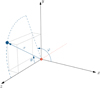 |
Figure 1 Cartesian and spherical coordinates with the drone (as red dot) at the origin. The dashed red line represents past trajectory. |
2.2.1 Compensating for motion
The recorded raw signals contain “distortions” of the emission signal due to the relative movement of the drone through space. These comprise the distance attenuation of the point source as well as the Doppler effect. Effects such as atmospheric sound absorption [19], which become relevant at longer distances, are not considered here.
From the trajectory, the distance rs,m from the drone (index s) to a microphone (index m) as well as the relative Mach number Mas,m can be calculated for each moment in time. Using these, the time signal recorded at the microphone can be shifted in time and its amplitude can be corrected, so as to synthesize a signal of a microphone positioned at a reference distance rs,0 and moving alongside the drone with varying azimuth and elevation:
 (10)
(10)
The time-dependent time-shift of the signal implicitly removes the frequency shift due to the Doppler effect.
For a signal recorded with a limited sampling rate, interpolation between samples may be necessary when implementing Equation (10).
2.2.2 Collecting directed energy
For the calculation of quantities describing radiation characteristics, an evaluation of the data in the frequency domain is useful. A continuous assignment of the signals to microphone channels, on the other hand, is not helpful due to the constantly changing relative angular position. Instead, a description of the signal according to radiation direction is much more practical.
In order to achieve this, the following signal processing is proposed:
Discretize the radiation direction space (φ, θ) around the drone into a number of segments.
Specify an FFT block length for transforming the data into the frequency domain.
Separate the time signal at each microphone into blocks of that length, which may overlap by a specified percentage.
At the beginning of each block, note the relative position (φ and θ) of the respective microphone to the drone.
Transform the data blocks into the frequency domain and assign them to the corresponding (φ, θ) segments.
The collected spectra are then averaged for each segment, yielding a single sound pressure value for each direction and frequency.
The flight path and sensor setup should be chosen so that samples can be collected for all desired angular positions of the discretized two-dimensional direction space. In this paper, two different discretizations, or sphere partitionings, are proposed. Both are easy to describe in the given spherical coordinate system.
For the first partitioning, the sphere is divided into segments with an equi-angular resolution in φ- and in θ-direction. As is shown in Figure 2, the result resembles the latitudes and longitudes of geographic coordinates. With a resolution of 32 angles in φ-direction and 16 angles in θ-direction, this equi-angular grid will be referred to as “EA512” in the remainder of the paper.
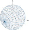 |
Figure 2 Partitioning of sphere into 32 × 16 sections with equal angle distribution (EA512 grid). |
While this grid allows a detailed and intuitive understanding of the 3D directivity, it does not convey the energy radiated towards the specific directions. This is because the area covered by one segment varies significantly from the poles to the equator. The spectra are averaged for each segment, so two segments with the same level but different areas do not actually contain the same energy. Furthermore, the actual directivity resolution is much higher at the poles than at the equator.
The second grid, shown in Figure 3, divides the sphere according to additional rules:
The cartesian axes should be located at the center of a segment.
For each plane spanned by two cartesian axes, the directivity should be describable by at least 8 evenly distributed angles.
All segments should span an equal surface so that the resulting sound pressures can be directly compared in terms of energy.
All possible directional angles should be accounted for.
There should be as few segments as possible.
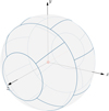 |
Figure 3 Partitioning of sphere into 18 sections with equal surface area (ES18 grid). |
An according partitioning with 18 segments can be achieved by
two polar caps with borders at θ = ψcap and θ = π − ψcap respectively,
a ring centered at the “equator” between θ = ψring and θ = π −ψring, with φ-equi-angular segmentation into 8 segments starting at
 , and
, andφ-equi-angular segmentation into 4 segments between the center ring and the caps, starting at

with  and
and  . The latitudinal center of the resulting 4-segment-rings does not lie exactly between equator and poles, but at 45.44° instead of 45° for positive z, thus slightly violating the uniform angle distribution of rule 2 (except for the xy plane). This equal-surface grid is referred to as “ES18”.
3 Application
The presented methods are applied to measured and simulated data in the following. In addition to investigating the general applicability of the described data processing, a major objective of this section is to determine whether a meaningful description of the sound emission is possible using the low-resolution ES18 grid alone.
3.1 General setup
The measurement was performed in a fully anechoic room at TU Berlin. The setup is depicted in Figure 4. The signals were recorded synchronously with 96 channels. 32 of the microphones are arranged in a multi-armed spiral and flush mounted in a plate parallel to the ground with a side length of 1.5 m. Their main purpose is to reconstruct the trajectory (see Sect. 2.1). The usability of a similar setup for flight path detection has been shown previously [12].
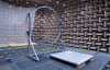 |
Figure 4 Measurement setup with the two arrays. Flight direction of the evaluated case is from right to left. |
The remaining 64 sensors are evenly distributed in an upright circle of approximately 2.1 m diameter. Signals from these microphones are mainly used for reconstructing the directed sound emission, as described in Section 2.2. Several of the microphones from the lower half of the circle are also used together with the plate microphones for trajectory detection.
The coordinate system is array-centered. Since the position of all microphones must be known, the relative positioning of the plate to the ring is important during setup. Apart from that, setting up the array in the measurement environment is not complex, since the two sub-arrays can be prepared in advance.
It is worth noting at this point that while it is necessary to have multiple synchronously recording channels, even a smaller number of microphones arranged to provide sufficient coverage of the angles of interest can yield meaningful results. Determining the minimum requirements is, however, beyond the intended scope of this paper.
The measured drone is a consumer quadcopter (shown in Fig. 5) that weighs 85 g, has a width of 17.5 cm, and a rotor diameter of 7.7 cm. Signals were recorded during a flight of the drone over the plate array through the array ring and beyond. The total signal duration evaluated in this paper is 3.9 s. The focus of this paper is on the amount of information that can be obtained from a single measurement. For a reliable and statistically sound characterization of the drone, evaluating repeated measurements would be necessary.
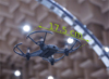 |
Figure 5 Drone used for the measurement. The rotor diameter is 7.7 cm. |
In Figure 6 the signal recorded by a single microphone, positioned between 7 and 8 o’clock in the ring array as shown in Figure 4, is depicted in the form of a spectrogram. Tonal components from the blade passing frequencies (BPFs) of the four rotors as well as some higher harmonics are clearly visible, as are minor broadband components. The drone passes the ring between seconds 2 and 3, where the measured sound pressure level is at its maximum of 43 dB at 637.5 Hz (12.5 Hz narrow band; for visibility purposes, the displayed levels are clipped at 30 dB in the figure).
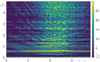 |
Figure 6 Single-channel spectrogram of the drone flight measurement. |
In the time section of the approaching drone, a superimposed interference pattern can be seen in the spectrogram. This is caused by reflections from the ground (i.e. the horizontal plate array and to a small extent the grate floor), also known as the acoustical Lloyd’s mirror effect [20]. The influence of this effect on the overall results is assumed to be small here and therefore not investigated further. For future measurements, it would be conceivable to make the setup environment fully absorbent or to consider a mirror source in the signal processing.
3.2 Trajectory reconstruction
For the flight path detection according to Section 2.1, the microphones on the plate as well as 17 channels from the lower part of the ring were used. The reason for omitting the other ring microphones is that the point spread function, i.e. the imaging of a point source through beamforming, of a fully circular array geometry exhibits strong side lobes [21]. This is undesirable because then a side lobe can be misidentified as the source position if the actual maximum does not lie exactly on a discretized focus grid point. Parameters for the calculation of the trajectory are summarized in Table 1.
Important parameters for the trajectory detection.
The accuracy of the localization is tested using reference measurements of a point source at three different positions in the plane of the upright microphone circle. The evaluated signal duration is 3 s and the chosen segment length for position detection is 0.1 s, resulting in 30 positional coordinates per measurement. Table 2 lists the detected averaged coordinates as well as the mean and the standard deviation of the position spread, i.e. the distances of the individual positions from their average. With a spread of less than 5 cm, the position reconstruction is shown to be reproducible within an acceptable tolerance.
Averaged detected coordinates of the three reference sources and spread (mean  and standard deviation sΔr).
The deviation of the reconstructed from the nominal source positions is documented in Table 3. The coordinate differences are of about the same order of magnitude as the source spread. The overall deviation of source 3 is higher than for the other two sources. Apart from possible inaccuracies in the documented nominal position of the source, the lower spatial separability of sources with increasing distance to the microphone array is a possible cause for the larger deviations. The influence of position uncertainties on the coordinates φ and θ as well as on the amplitude correction decreases with increasing distance of the source position, so that at larger distances, higher tolerances in position determination are acceptable.
Deviation of averaged detected to nominal coordinates of the reference sources.
The reconstructed flight path with a duration of 3.9 s is shown in Figure 7. Even though the drone was remotely steered to follow a straight path, altitude variations are clearly visible. The reason for these is mainly the drone relying on its optical sensors to control its altitude and being challenged with uneven terrain due to the setup. This trajectory is used as basis for the further evaluations.
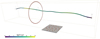 |
Figure 7 Reconstructed trajectory of the drone flight with velocities. Red dots represent microphone positions. The moving coordinate system is indicated at three instants in time (start, array passing, end). The yellow frame indicates the 3D focus area (i.e. the monitored flight corridor) evaluated for recovering the trajectory from the microphone array. |
3.3 Simulated sources
In addition to the measurement, two simulated datasets were generated: one of a moving monopole, the second of a moving dipole. As with the evaluations in this paper, the simulations of the datasets were done using the Python software package Acoular [22, 23].
The time signals of the sources are chosen to be the same for both datasets and to roughly resemble the signal of a quadcopter drone. The dipole lobes of maximum radiation are oriented perpendicular to the ground, so that a sensor positioned directly above the source would record the exact same signal for the monopole and the dipole.
The array setup is identical to the one used in the measurement, except for the simulations being free of reflections, sensor directionalities, or flow effects. The simulated flight paths correspond exactly to the reconstructed trajectory of the measured drone. For brevity, the three evaluated datasets are hereafter referred to as described in Table 4.
Abbreviations of the three datasets.
Figure 8 shows the spectrum calculated from the moving monopole at a single channel and averaged over the entire measurement time, as well as the spectrum of the signal after motion correction according to Section 2.2.1. After dedopplerization, the tonal peaks are a lot more distinct, since the energy distribution over adjacent frequency bands due to the pitch shift is reversed. Furthermore, the broadband noise level is increased from about 48 dB in the raw data to about 55 dB in the corrected signal due to the compensation of the sound path and normalization to 1 m reference distance.
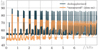 |
Figure 8 Narrow band spectrum (Δf = 6.25 Hz) of the simulated moving monopole. |
3.4 Directivity mapping
Since the directional information is acquired sequentially, it is important that the sound emission is as homogeneous over time as possible, so that the sound pressure data can be compared between different angles. Even with a straight trajectory, this is not always feasible, as can be seen from the varying rotor BPFs in Figure 6.
As mentioned above, one possible way to obtain representative results is the evaluation of multiple measurements with the same drone and flight mode. Other ways to increase the sample number for averaging are:
decreasing the FFT block size,
increasing the overlap of the FFT blocks,
using multiple discrete frequency bands,
increasing the number of directions that are grouped.
The last point can be realized, for example, by increasing either the number of sensors or the size of the segments (i.e. decreasing the number of sphere partitions). This is visualized in Figures 9b and 9c, where the number of short-time spectra used for averaging the sound pressure data in each segment is shown for the two used sphere partitionings. When using the ES18 grid, there are approximately 30 to more than 50 times as many samples available per segment as when using the EA512 grid for the evaluation.
 |
Figure 9 Latitudinal angle timeline of the ring microphones in the drone’s coordinate system (a) and histograms of how many short-time spectra are calculated per respective grid segment (b, c). |
The θ-angles covered during the flight are shown in Figure 9a. With the chosen ring array geometry, the time during which data can be collected for emission angles around  is a lot shorter than the time the microphone positions relative to the drone is close to the poles of the sphere grids. As the drone at no point of its trajectory directly flies towards a microphone, the angles θ = 0 and θ = π are not covered. The imbalance in the distribution of latitude angles can also be seen in the histograms, where the differences between sectors with the most samples and those with the fewest samples are several orders of magnitude. In the case of the EA512 grid with high angular resolution (Fig. 9b), no samples could be collected for several positions near the poles.
Assuming that all emission angles are of similar interest, a more uniform angular coverage would be preferable. This could be achieved by positioning microphones along and around the trajectory rather than in a single ring. Important parameters used for the sample collection and signal processing in this paper are listed in Table 5.
Important parameters for the directed sample collection.
3.4.1 EA512 high-resolution visualizations
In Figures 10–12, the collected directional sound emission (sound pressure level at 1 m distance) is plotted against the longitudinal angle φ and the latitudinal angle θ with a dynamic range of 15 dB. For a more intuitive understanding, the values are also plotted in a 3D perspective. Here, the distance from the origin represents the relative sound pressure level.
 |
Figure 10 Simulated monopole: visualization of the directional sound radiation using the EA512 grid, evaluated for two octave bands. |
In Figure 10, the reconstructed emission for the simulated moving monopole is shown for the octave bands around 500 Hz and 2 kHz. The omnidirectional characteristic is clearly visible, however, at 500 Hz, the variation across the direction is larger than at 2 kHz. This is explained by the above-mentioned number of averaging samples (in this case, discrete narrow frequency bands) being lower in case of the 500 Hz octave.
This is also visible for the simulated dipole case evaluated for the same frequency bands (shown in Fig. 11): The reconstruction of the dipole characteristic with orientation along the y-axis is much smoother for the 2 kHz octave band. The evaluation and visualization of the simulated datasets show that with this data processing, it is possible to reconstruct detailed directivity information if the trajectory of the source is known.
 |
Figure 11 Simulated dipole: visualization of the directional sound radiation using the EA512 grid, evaluated for two octave bands. |
Figure 12 shows a corresponding visualization of the measured data from the drone flight for octave bands from 500 Hz to 16 kHz. For higher frequencies, the exhibited directivity is similar to that of the dipole, with more energy emitted in positive and negative y direction. While this general characteristic is to be expected [2], additional effects are visible here.
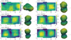 |
Figure 12 Measured drone: visualization of the directional sound radiation using the EA512 grid, evaluated for six octave bands. |
For one, the lobes are tilted, so that the upper lobe is directed slightly towards the flight direction. This can be expected, since the drone itself is slightly tilted in that direction while flying. Also, the amount of energy radiated up- and downwards is not identical and depends on the regarded frequency band, For the evaluated octave band around 500 Hz, the directivity appears to be considerably different in that most of the energy is radiated in lateral direction.
Furthermore, for some octave bands and best visible at 4 kHz, the directivity pattern is shown to be elongated in z (i.e. flight) direction. From these evaluations, it cannot be said with certainty whether this is a physical effect or if this is caused by small deviations of the assumed (i.e. reconstructed) to the actual trajectory.
In all considered frequency bands, more sound energy is detected to be radiated directly in the direction of flight (θ close to zero) than in the opposite direction. A possible explanation for this are emission reflections at the array plate on the ground, which are not considered in the evaluation and will be assumed to originate directly from the drone.
3.4.2 Evaluation with the ES18 grid
Evaluating the directed sound emission using the ES18 sphere partitioning has the advantage that a higher number of samples can be used for averaging the sound pressure level within a segment. This comes at the cost of a decreased angular resolution. The suitability of the ES18 grid for generating meaningful results is investigated in the following.
Figure 13 shows the sound radiation in all discretized directions of the sphere. Major phenomena visible in Figure 12 can be seen here as well: a dipole-like directivity, the tilting of the lobes, and the increased level in the segment pointing in flight direction. This indicates that a discretization with the lower-resolution ES18 grid allows a sufficient reconstruction of important emission characteristics.
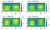 |
Figure 13 Directional sound radiation of the drone, evaluated with the ES18 partitioning for several octave bands. |
A quantitative comparison of the results for both grids is shown in Figure 14 for the simulated dipole and the measured drone in the xy plane. The directivity reconstructions are in good agreement for most angles discretized by both grids. However, for φ = 0° and φ = 180°, the levels are higher for the ES18 grid, because the broader longitudinal range represented by these angles includes directions into which more energy is radiated.
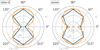 |
Figure 14 Directivity patterns (sim-d and msm) in the xy plane for the 4 kHz octave band, displayed dynamic 15 dB, blue: ES18, orange: EA512. |
In case of the simulated moving monopole, the reconstructed levels are in agreement for both grid types. This is shown in Figure 15, which also features the directivity patterns on the ES18 grid for different frequencies. As is expected with a monopole, the directivity results for the xy, zx and zy planes are virtually identical.
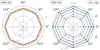 |
Figure 15 Directivity patterns in the xy plane (blue: ES18, orange: EA512) for 4 kHz, and in the perpendicular planes for octave bands from 500 Hz to 8 kHz (shades from light to dark). |
Directivity patterns in the planes perpendicular to the three coordinate axes are shown in Figure 16 for the simulated dipole and the measured drone at different frequencies. Even though the dipole is simulated to be perfectly symmetric, the visualization shows a different directivity in the flight than in lateral direction. This can best be seen when comparing sub-figures “sim-d, xy” and “sim-d, zy”, which should be identical. The reason for the differences lies in the between-the-axes segments of the ES18 grid being of considerably different shape for the two cases (see also Fig. 3), thus grouping a different set of relative angles to represent the respective emission direction. While the dipole directivity representation would appear more realistic if the sphere segmentation were done differently (e.g. by choosing an orientation of the poles along the y axis), arbitrary and highly varying directivities can easily lead to misrepresentations if too few segments are chosen for discretization.
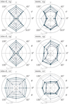 |
Figure 16 ES18 directivity patterns in different planes for the simulated dipole and the measured drone for octave bands from 500 Hz to 8 kHz (shades from light to dark). Displayed dynamic is 15 dB below max. |
Nevertheless, the ES18 grid can be used to obtain a general overview of the emission characteristics in a simple way, as can be seen from the drone measurement in the right column of Figure 16. The emission characteristics discussed in Figures 12 and 13 are also visualized here, with the polar diagram allowing an intuitive interpretation.
3.5 Sound power and directivity factor
In the context of acoustic characterization of machinery, it is often desirable to derive easily comparable quantities from measurements. An example for this is the calculation of the sound power level using the enveloping surface method, e.g. described in ISO 3744 [3]. With the sound power W being defined as the integral of the sound intensity over the surrounding surface, it can be calculated via
 (11)
(11)
where N is the number of elements in a surface discretization, i.e. in the case here, the segments of the two sphere partitionings. For the EA512 grid, the surface Si of the segments depends on the respective latitude. In contrast, the segments in the ES18 grid all have a surface of Si,18 = 4πr2/18, which leads to the squared sound pressure  being the only varying term in the summation of Equation (11). The properties of the medium in which the sound propagates are described by the density ρ0 and the speed of sound c.
Since drones, as shown above, are highly directional sound sources, it is convenient to quantify the directivity in a value as well. This is possible with the directivity factor Q, which sets the sound intensity in a selected reference direction in relation to the average intensity of the source [24]:
 (12)
(12)
The sphere radius r = 1 m corresponds to the distance to which all sound pressures are normalized. As the radiation of the drone towards the ground is deemed to be of major importance, the reference direction here is selected to be the negative y axis, with  being the prms value representative for this direction. For the EA512 grid,
  is calculated by averaging the prms values of the four segments adjacent to this axis.
In case of the ES18 grid, a representative sphere segment can be directly selected. Furthermore, for 18 segments with the same surface area, Equation (12) simplifies to:
 (13)
(13)
Figure 17 shows the frequency-dependent directivity factor for the two simulated cases. In case of the monopole, Q varies around and close to a value of one, which indicates an omnidirectional radiation. The dipole has an average  , which comes close to a directivity factor of 3 for a perfect dipole [24]. For both cases, the average values calculated using the different sphere partitionings are in good agreement, whereas the standard deviation is about twice as high when using the EA512 grid as compared to the ES18 grid.
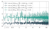 |
Figure 17 Frequency-dependent directivity factor of the simulated sources. |
These are simulated cases where variations in directivity indicate imperfect reconstruction caused, for example, by insufficient averaging. Therefore, the displayed deviations from the average value are a good measure for the capabilities of the methods.
The directivity factor for the measurement is shown in Figure 18. As with the simulations, the variation of Q is higher if the emission reconstruction is done on the EA512 instead of the ES18 grid. The general shape of the curve is similar for both grids. In contrast to the simulated cases, the directivity visibly depends on the frequency. The low directivity factor at 500 Hz corresponds to the flattened shape seen at this frequency in Figure 12.
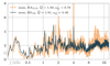 |
Figure 18 Directivity factor of the measured drone. |
While a directivity of 4 and even above is observed at some frequencies, for the most part Q is well between the directivities of a monopole and a dipole, with an average factor af about  . The average directivity factors and their standard deviation for all cases and grids are summarized in Table 6.
Calculated directivity factor average  and standard deviation sQ.
Figure 19 shows the reconstructed sound power spectrum of the measured drone. The results calculated on the two different grids are in good agreement, with no significant deviations. The spectrum exhibits strong tonal components, with he highest peaks being observed between 500 Hz and 2 kHz. In addition to the spectrum, the total as well as the A-weighted sound power level [25] are calculated for convenience and to illustrate that similar results can be obtained with the array-based evaluation presented here as with stationary measurements.
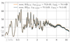 |
Figure 19 Narrow-band sound power spectrum (Δf = 12.5 Hz) of the measured drone. |
Table 7 compiles the weighted and unweighted sound power levels for the simulated and measured cases. The direct comparison of the values calculated using EA512 and ES18 with a maximum difference of 0.3 dB shows that the choice of either of the two grids is not significant for the calculation of the sound power level.
Calculated sound power levels.
4 Conclusion
The purpose of the investigations conducted here is to demonstrate the principal applicability of array measurements for an emission-based characterization of a small-scale drone in cruise mode. The presented methods have been shown to be suitable for that and enable the determination of the sound power and directivity of the drone. Using simulated datasets, the applicability of the proposed signal processing could be verified.
Two grids with different spatial resolutions were proposed for investigating the directional radiation. Both grids are suitable for deriving the quantities of interest. With the low-resolution ES18 grid, both the general directivity and derived quantities can be determined with sufficient accuracy. Applying the EA512 grid is useful when more detailed information about the directional radiation is needed, although at the cost of less data available for averaging.
The microphone array used for the investigations is easy to set up and the sensor arrangement proved to be capable of providing the drone’s trajectory and its emission characteristics. However, for a more uniform sampling of the directional radiation, it would be advantageous if the microphones were distributed more along the flight path. Furthermore, for future studies it would be desirable to either change the measurement environment so that no unwanted reflections occur or that reflections be taken into account in the signal processing.
For a reliable acoustic characterization of the drone’s emission, evaluating only one fly-by is not sufficient, since the sound radiation varies along the flight path. The remedy here is several measurements of the same drone operated in a comparable flight mode, and a subsequent averaging of the results.
Conflict of interest
The author declares that he has no conflicts of interest in relation to this article.
Acknowledgments
Thanks are due to: Paul Testa and Tobias Jüterbock for their help with the setup and execution of the drone measurement, the contributors to the Acoular software package, on which the signal processing done for this paper heavily relies, and to Ennes Sarradj and the TU Berlin Department of Engineering Acoustics, where the experiment was carried out. The publication of this article is supported by the Open Access Publication Fund of TU Berlin.
References
- United States Department of Transportation, Federal Aviation Administration: FAA Aerospace Forecast – Fiscal Years 2021–2041, 2021. Available at https://www.faa.gov/data_research/aviation/aerospace_forecasts/. [Google Scholar]
- B. Schäffer, R. Pieren, K. Heutschi, J.M. Wunderli, S. Becker: Drone noise emission characteristics and noise effects on humans – a systematic review. International Journal of Environmental Research and Public Health 18 (2021) 11. [Google Scholar]
- ISO: ISO 3744:2010 – Acoustics – Determination of sound power levels and sound energy levels of noise sources using sound pressure – Engineering methods for an essentially free field over a reflecting plane, 2010. https://www.iso.org/standard/52055.html. [Google Scholar]
- The European Commission: Commission Delegated Regulation (EU) 2019/945 of 12 March 2019 on unmanned aircraft systems and on third-country operators of unmanned aircraft systems. Official Journal of the European Union 62 (2019) 1. https://eur-lex.europa.eu/eli/reg_del/2019/945/oj. [Google Scholar]
- K. Cussen, S. Garruccio, J. Kennedy: UAV noise emission – A combined experimental and numerical assessment. Acoustics 4 (2022) 297–312. [CrossRef] [Google Scholar]
- ICAO: Annex 16 to the Convention on international civil aviation, Environmental protection. Volume I – Aircraft noise. 5th edition, incorporating amendments 1-9, International Civil Aviation Organization, 2008. https://store.icao.int/en/annex-16-environmental-protection-volume-i-aircraft-noise. [Google Scholar]
- DIN: DIN 45643 – Messung und Beurteilung von Fluggeräuschen, Beuth Verlag GmbH, 2011. https://doi.org/10.31030/1737047. https://www.beuth.de/de/norm/din-45643/136846081. [Google Scholar]
- I. González-Hernández, S. Salazar, R. Lozano, O. Ramírez-Ayala: Real-time improvement of a trajectory-tracking control based on super-twisting algorithm for a quadrotor aircraft. Drones 6 (2022) 36. [CrossRef] [Google Scholar]
- Y.I. Abdel-Aziz, H.M. Karara, Michael. Hauck: Direct linear transformation from comparator coordinates into object space coordinates in close-range photogrammetry. Photogrammetric Engineering & Remote Sensing 81 (2015) 103–107. [CrossRef] [Google Scholar]
- C. Hui, C. Yousheng, W.W. Shing: Trajectory tracking and formation flight of autonomous UAVs in GPS-denied environments using onboard sensing, in Proceedings of 2014 IEEE Chinese Guidance, Navigation and Control Conference, IEEE, 2014, pp. 2639–2645. [CrossRef] [Google Scholar]
- X. Chang, C. Yang, J. Wu, X. Shi, Z. Shi: A surveillance system for drone localization and tracking using acoustic arrays, in 2018 IEEE 10th Sensor Array and Multichannel Signal Processing Workshop (SAM), IEEE, 2018, pp. 573–577. [CrossRef] [Google Scholar]
- G. Herold, A. Kujawski, C. Strümpfel, S. Huschbeck, M.U. de Haag, E. Sarradj: Flight path tracking and acoustic signature separation of swarm quadcopter drones using microphone array measurements, in Quiet Drones 2020 – International e-Symposium on UAV/UAS Noise, Paris, France, 2020, pp. 1–9. [Google Scholar]
- P.D. Welch: The use of fast Fourier transform for the estimation of power spectra: a method based on time averaging over short, modified periodograms. IEEE Transactions on Audio and Electroacoustics 15 (1967) 70–73. [CrossRef] [Google Scholar]
- R. Merino-Martínez, P. Sijtsma, M. Snellen, T. Ahlefeldt, J. Antoni, C.J. Bahr, D. Blacodon, D. Ernst, A. Finez, S. Funke, T.F. Geyer, S. Haxter, G. Herold, X. Huang, W.M. Humphreys, Q. Leclère, A. Malgoezar, U. Michel, T. Padois, A. Pereira, C. Picard, E. Sarradj, H. Siller, D.G. Simons, C. Spehr: A review of acoustic imaging methods using phased microphone arrays. EAS Aeronautical Journal 10 (2019) 197–230. [CrossRef] [Google Scholar]
- R.P. Dougherty: Functional beamforming, in Proceedings of the 5th Berlin Beamforming Conference (2014) 1–25. [Google Scholar]
- R.P. Dougherty: Beamforming in acoustic testing, in T.J. Mueller, Ed. Aeroacoustic measurements. Berlin, Heidelberg: Springer, 2002, pp. 62–97. [CrossRef] [Google Scholar]
- E. Sarradj: Three-dimensional acoustic source mapping with different beamforming steering vector formulations. Advances in Acoustics and Vibration 2012 (2012) 1–12. [CrossRef] [Google Scholar]
- B.D.O. Anderson, J.B. Moore: Optimal filtering, Prentice-Hall, Englewood Cliffs, NJ, 1979. [Google Scholar]
- ISO. ISO 9613–1:1993 – Acoustics – Attenuation of sound during propagation outdoors – Part 1: Calculation of the absorption of sound by the atmosphere. https://www.iso.org/standard/17426.html. [Google Scholar]
- W.M. Carey: Lloyd’s mirror – Image interference effects. Acoustics Today 5 (2009) 2. [Google Scholar]
- E. Sarradj: A generic approach to synthesize optimal array microphone arrangements, in Proceedings of the 6th Berlin Beamforming Conference, 2016, pp. 1–12. [Google Scholar]
- E. Sarradj, G. Herold: A Python framework for microphone array data processing. Applied Acoustics 116 (2017) 50–58. [CrossRef] [Google Scholar]
- E. Sarradj, G. Herold, S. Jekosch, A. Kujawski, M. Czuchaj: Acoular, 2021. https://zenodo.org/record/4740537 [Google Scholar]
- L.L. Beranek, T.J. Mellow: Acoustics: Sound fields and transducers. Elsevier, 2012. [Google Scholar]
- IEC: IEC 61672–1:2013 – Electroacoustics – Sound level meters – Part 1: Specifications. https://standards.iteh.ai/catalog/standards/clc/7de04d56-6445-4410-a810-0e5216645fb6/en-61672-1-2013. [Google Scholar]
Cite this article as: Herold G. 2022. In-flight directivity and sound power measurement of small-scale unmanned aerial systems. Acta Acustica, 6, 58.
All Tables
Averaged detected coordinates of the three reference sources and spread (mean and standard deviation sΔr).
All Figures
|
Figure 1 Cartesian and spherical coordinates with the drone (as red dot) at the origin. The dashed red line represents past trajectory. |
| In the text | |
|
Figure 2 Partitioning of sphere into 32 × 16 sections with equal angle distribution (EA512 grid). |
| In the text | |
|
Figure 3 Partitioning of sphere into 18 sections with equal surface area (ES18 grid). |
| In the text | |
|
Figure 4 Measurement setup with the two arrays. Flight direction of the evaluated case is from right to left. |
| In the text | |
|
Figure 5 Drone used for the measurement. The rotor diameter is 7.7 cm. |
| In the text | |
|
Figure 6 Single-channel spectrogram of the drone flight measurement. |
| In the text | |
|
Figure 7 Reconstructed trajectory of the drone flight with velocities. Red dots represent microphone positions. The moving coordinate system is indicated at three instants in time (start, array passing, end). The yellow frame indicates the 3D focus area (i.e. the monitored flight corridor) evaluated for recovering the trajectory from the microphone array. |
| In the text | |
|
Figure 8 Narrow band spectrum (Δf = 6.25 Hz) of the simulated moving monopole. |
| In the text | |
|
Figure 9 Latitudinal angle timeline of the ring microphones in the drone’s coordinate system (a) and histograms of how many short-time spectra are calculated per respective grid segment (b, c). |
| In the text | |
|
Figure 10 Simulated monopole: visualization of the directional sound radiation using the EA512 grid, evaluated for two octave bands. |
| In the text | |
|
Figure 11 Simulated dipole: visualization of the directional sound radiation using the EA512 grid, evaluated for two octave bands. |
| In the text | |
|
Figure 12 Measured drone: visualization of the directional sound radiation using the EA512 grid, evaluated for six octave bands. |
| In the text | |
|
Figure 13 Directional sound radiation of the drone, evaluated with the ES18 partitioning for several octave bands. |
| In the text | |
|
Figure 14 Directivity patterns (sim-d and msm) in the xy plane for the 4 kHz octave band, displayed dynamic 15 dB, blue: ES18, orange: EA512. |
| In the text | |
|
Figure 15 Directivity patterns in the xy plane (blue: ES18, orange: EA512) for 4 kHz, and in the perpendicular planes for octave bands from 500 Hz to 8 kHz (shades from light to dark). |
| In the text | |
|
Figure 16 ES18 directivity patterns in different planes for the simulated dipole and the measured drone for octave bands from 500 Hz to 8 kHz (shades from light to dark). Displayed dynamic is 15 dB below max. |
| In the text | |
|
Figure 17 Frequency-dependent directivity factor of the simulated sources. |
| In the text | |
|
Figure 18 Directivity factor of the measured drone. |
| In the text | |
|
Figure 19 Narrow-band sound power spectrum (Δf = 12.5 Hz) of the measured drone. |
| In the text | |
Current usage metrics show cumulative count of Article Views (full-text article views including HTML views, PDF and ePub downloads, according to the available data) and Abstracts Views on Vision4Press platform.
Data correspond to usage on the plateform after 2015. The current usage metrics is available 48-96 hours after online publication and is updated daily on week days.
Initial download of the metrics may take a while.