| Issue |
Acta Acust.
Volume 8, 2024
|
|
|---|---|---|
| Article Number | 4 | |
| Number of page(s) | 12 | |
| Section | Computational and Numerical Acoustics | |
| DOI | https://doi.org/10.1051/aacus/2023068 | |
| Published online | 16 January 2024 | |
Technical & Applied Article
Efficient calculation of the three-dimensional sound pressure field around a slab track
Chalmers University of Technology, Division of Applied Acoustics, Department of Architecture and Civil Engineering, Sven Hultins Gata 8a, 41258 Gothenburg, Sweden
* Corresponding author: This email address is being protected from spambots. You need JavaScript enabled to view it.
Received:
27
February
2023
Accepted:
17
December
2023
Abstract
The wavenumber domain Boundary Element (2.5D BE) method is well suited to calculate the acoustic sound field around structures with a constant cross-section along one dimension, such as noise barriers or railway track. By expressing the sound field along this dimension in wavenumber domain, the numerical model is reduced from a 3D model to 2D model at each wavenumber. A consequence of the required discrete Fourier domain representation is that the sound field is represented by periodically repeating sections, of which only one section is physically meaningful. The resolution and the number of required wavenumbers increases with the desired length and spatial discretisation of this section. Describing the sound field adequately to auralise the sound without disturbing artefacts requires a large number of wavenumbers (and thus 2D BE computations), which is not feasible for large geometries. Here, a method is introduced that allows the calculation of the 3D sound field by solving a single 2D BE problem for a dense frequency spectrum and interpolating at higher wavenumbers. The calculation efficiency is further increased by precalculating the acoustic transfer functions between each BE surface element and receiver positions. Combining these two methods allows for efficient calculation of the 3D sound field around acoustically rigid structures such as slab tracks. The numerical approach is validated by comparison with a standard 2.5D BEM calculation and an analytical solution. Precalculated transfer functions to calculate the sound radiation from railway track, which are made available online, are illustrated. An example application is presented.
Key words: 2.5D BE / Acoustic sound field / Acoustic transfer functions / Numerical methods / Railway track
© The Author(s), Published by EDP Sciences, 2024
 This is an Open Access article distributed under the terms of the Creative Commons Attribution License (https://creativecommons.org/licenses/by/4.0), which permits unrestricted use, distribution, and reproduction in any medium, provided the original work is properly cited.
1 Introduction
With the growing transport needs and the intended shift towards more sustainable modes of transport, the noise from railway operations is expected to increase [1]. Rolling noise due to vibrations on the track and wheels dominates the noise in a wide range of vehicle speeds [2]. Estimating the noise radiated from operations on new tracks or the effect of introducing abatement measures on existing tracks has been of interest to both the scientific community and railway operators for several decades. Starting with analytical models, such as, for example, presented by Remington [3], the requirements on and the complexity of such predictive models have continuously grown in parallel to the computational possibilities. Thompson et al. [4] used point-dipole sources to represent the radiation of a rail in free space and investigated its directivity. This approach was continued by Zhang et al. [5], where the effect of discrete support and proximity to the ground was included using line multipole sources and quadrupoles in each sleeper span.
A prevalent numerical approach to calculate the radiation from the rail is the Wavenumber domain Boundary Element method (2.5D BE), an adapted Boundary Element method in which one dimension is decomposed into a wavenumber spectrum [6–11]. The 3D geometry is reduced to a 2D geometry. 2D BE problems then need to be solved for each wavenumber in the spectrum. The computational cost increases proportionally with the number of 2D BE calculations, and is thus a function of the required resolution and the upper limit of the wavenumber and frequency spectra.
The computational cost increases proportionally to the number of 2D BE calculations, which itself depends on the resolution and the upper limit of both spectra. The upper limit is determined by the required temporal and spatial resolutions. Nilsson et al. [8] point out that in the case of radiation from a rail, whose vibration is typically dominated by few propagating waves, the wave numbers can be spaced more closely to these waves to increase efficiency in the calculation. Still, for other applications and for a desired high spatial and temporal resolution of the sound field, the computational cost of the standard 2.5D method can be infeasible. A high spatial and temporal resolution is, for example, necessary when aiming for a time-domain calculation of the sound field quantities. A time-domain approach allows, among others, the calculation of peak levels, squealing noise amplitudes, the acoustic effect of a wheel flat or a rail joint, or other transients in rolling noise. The need to develop a time-domain model for the prediction of transient noise has been pointed out by Torstensson et al. [12] and Nielsen et al. [13].
Here, we describe an extension of the 2.5D BE method to calculate the 3D sound field generated by the vibration of railway tracks. This sound field is calculated efficiently in a resolution adequate to, for instance, modelling a pass-by of a moving force in the time domain. Note that a similar method is used by Li et al. [14] for predicting the low-frequency radiation from concrete bridges. However, in [14], radiation is precalculated per bridge mode instead of per BE node, and the analysis is limited to the frequency range up to 1000 Hz. The presented method is limited to acoustically hard surfaces, and absorption is not considered.
The computational efficiency is addressed in two ways. First, a geometric relation is used between the wavenumber in air and the wavenumber along the track to avoid the need to solve the BE problem for each combination of wavenumber and frequency. Instead, the BE-problem only needs to be solved for the lowest wavenumber in the spectrum. Then, the BE-result at any higher wavenumber can be derived by an interpolation operation. Essentially, the 3D sound field can be calculated for the cost of a 2D sound field, plus an interpolation operation. This reduces the computational cost when using the 2.5D BE method.
Second, acoustic transfer functions are precalculated for common acoustic geometries such as a rail in acoustic free space and half space, a rail above a track surface, and a track and train combination. Once accomplished, this replaces the need for solving the BE-problem with a simple multiplication and summation operation. These two approaches are presented in Sections 2 and 3, respectively. A validation of the first approach is presented in Section 2.2. In Section 3.2, four acoustic geometries are introduced for which the transfer functions have been precalculated. An example of these transfer functions is discussed for illustration. The calculation procedure is available online in an open-source Python package [15], which allows the calculation of the sound pressure at several points, as well as the total radiated sound power for given surface velocity data. The corresponding acoustic transfer functions are available online [16].
2 Calculating the 3D sound field from a 2D BE solution
This section introduces the first approach to reducing the numerical cost and presents a validation.
2.1 Method
The approach to calculating the 3D sound field is based on the 2.5D BE method [8]. The 2.5D BE method is well suited for geometries that are approximately constant in one dimension. The constant geometry in the cross-section allows discretising the sound field in the wavenumber domain and reduces the 3D BE problem to 2D problems at each wavenumber.
Figure 1 shows the cross-section of a rail located in the y, z-plane, which is assumed to be constant along the x direction. A wavenumber vector K0 in the air is indicated by the orange arrow. It can be expressed as the sum of the vectors of the component in the plane (α) and the component in the x-direction (κ0). A second wavenumber vector Kn is indicated in green, with the same projection on the y, z-plane and a component along the x-direction κn. The 2D Helmholtz integral equation for an unbounded exterior problem is
 (1)in which the integral is evaluated over the boundary Γ, with the density in air ρ, the surface normal velocity vn, the surface pressure p, and the angular frequency ω = 2πf. The variable Ψ represents the fundamental solution to the 2D Helmholtz equation at the point P, with
 (2)and its derivative in the surface normal direction n,
 (3)where
  is the Hankel function of the second kind and order zero and
  is of first order. The coefficient C(P) is equal to 1 for P in the acoustic domain and 1/2 on a smooth boundary. The integral equation is solved element-by-element by discretisation and collocation. Detailed derivation and implementation strategies are presented, for example, by Wu [17].
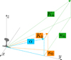 |
Figure 1 Projection of two wavenumbers K0 and Kn in air on the y, z-plane and the corresponding longitudinal components κ0 and κn, respectively. |
The two terms in the Helmholtz integral equation, evaluated on an element-by-element basis, form two matrices H and G with one column per element and one row per collocation point. These form the global system of equations,
 (4)with the vectors
  and
and  collecting the nodal pressures and normal surface velocities, one of which is known for each node. The system of equations is sorted according to the known and unknown boundary conditions. The combined Helmholtz integral equation formulation (CHIEF) is used to avoid cavity resonances, leading to additional equations. The system is solved using a least-squares solver.
In the standard implementation of this method, this 2D BE problem is solved for each combination of frequency f and wavenumber κn. The resolution and limits for the f- and κ-spectra are chosen based on the desired temporal and spatial limits and resolution. However, this requires solving many 2D BE problems, which is inefficient and, for large geometries, infeasible at high frequencies. Using the relationship between the wavenumber in the air and its projection in the 2D plane for each wavenumber and frequency, this need can be eliminated when neglecting absorption and only considering acoustically hard surfaces. For each frequency f, the magnitude of the wavenumber vector in the air K is
 (5)
(5)
As shown in Figure 1, for each wavenumber along the track κ, this wavenumber vector in air K can be expressed as a component α in the 2D plane that contains the y- and z-axes,
 (6)and a component κ in x-direction along the waveguide. Notice that the wavenumber vector in air K and the longitudinal wavenumber κ are independent, as they are a consequence of the chosen discretisation of the frequency and wavenumber domains, respectively.
For each combination of κ and the wavenumber vector in the air K, there is exactly one α in the 2D plane. However, a given α can be the result of infinitely many combinations of κ and K. Figure 1 shows two combinations of κ and K (κ0, K0 and κn, Kn) which share the same α. This is true if
 (7)or, using equation (5) and rearranging for f0,
 (8)
(8)
This relation can be used by first evaluating equation (4) for a dense frequency spectrum in combination with a small wavenumber κ0. Then, for higher wavenumbers κn, equation (8) maps any frequency to a frequency in the dense original spectrum at which the α in the 2D plane is identical. The calculated frequency f0 is likely not part of the precalculated dense spectrum, and an interpolation operation is necessary in the frequency domain. In other words, at each wavenumber except for the lowest wavenumber, the operation of solving the 2D BE problem for each frequency in the spectrum can be replaced by a complex interpolation operation. Note that a sufficiently dense original frequency spectrum is necessary, even when evaluating only at a few frequency lines per octave band, as equation (8) non-linearly maps to frequency lines in between the original ones.
A standard implementation of the complex quadratic interpolation is used, interpolating the real and imaginary part seperately (see, e.g., interp1 in MATLAB or interp in Numpy). Only real-valued frequencies are used as query points. Introducing absorption would require introducing complex frequencies as query points. In that case, the original spectrum would need to be precalculated for half the complex plane defined by 0 ≤ real(f0) ≤ fmax and −fmax ≤ imag(f0) ≤ fmax. Since this approach is less efficient (cf. Sect. 4.1), we here focus on acoustically hard surfaces.
To avoid extrapolation, any query point at which to evaluate the interpolation needs to lie between the limits of the original spectrum. Conveniently, this requirement is already fulfilled by the method itself. Figure 2 visualises the relationship between fn and f0 for the whole wavenumbers from 0 rad/m to 10 rad/m in the frequency range 0–1000 Hz. From equation (8) follows that for κn > κ0, the frequency f0 is strictly smaller than a frequency fn with the same α in the 2D plane. Therefore, a frequency spectrum at any higher wavenumber maps to smaller frequency lines, and thus the upper bound is fulfilled. The lower bound is limited by the physical properties of sound radiation. Figure 2 shows that for increasing wavenumbers, increasing frequencies get mapped to 0 Hz in the f0 spectrum. Physically, this is because for these combinations of kn and Kn, the wavenumber in the air is smaller than the wavenumber along the track, so no projection on the 2D plane is possible. Mathematically, this is a consequence of the expression under the root in equation (8), which becomes negative for
 (9)which for
  can not be fulfilled for real κ. For imaginary wavenumbers κ, radiation occurs only in the near field, and no sound power is radiated. These wavenumbers are excluded from further calculations.
 |
Figure 2 Mapping between fn and f0 for selected whole wavenumbers κn 0 rad/m to 10 rad/m. |
The method described above establishes a relationship between a given α and combinations of κ and K. For a given α, the phase relation between all the source elements and the receiver points is established in the BE formulation. However, there is a relevant frequency-dependent scaling of the magnitude in the 2D Helmholtz integral equation (Eq. (1)), as the first term of the integral contains the factor jω and the normal velocity vn. A scaling of the boundary element equation (4) is proposed,
 (10)such that this frequency dependency is instead included in the normal velocity. The scaling of
  can be introduced before or after the solution of the BE problem. Scaling does not affect the type of boundary conditions that can be used. If boundary conditions other than the Neumann boundary condition are used, the elements in the result vector corresponding to a normal velocity need to be scaled accordingly.
In summary, the 3D sound field of a structure with constant cross-section can be calculated in the frequency-wavenumber domain by
describing the acoustic boundaries and -domain by standard 2D boundary elements,
selecting an appropriate discretisation of the wavenumber and frequency domain,
solving the 2D BE problem for each frequency in the selected spectrum at the lowest wavenumber in the spectrum k0,
for each larger wavenumber kn and for each frequency:
This first approach makes it possible to solve the 2D BE problem for only one wavenumber at every frequency in a dense frequency spectrum and then generates solutions at higher wavenumbers by interpolation and frequency-dependent magnitude scaling of the result. A 2D inverse Fourier transform of the form
 (11)is used to calculate the signal in spatial and temporal domain. Note that positive and negative κ produce identical values for α in equation (6), which means that for a symmetric excitation spectrum (vn(κ) = vn(−κ)), the pressure spectrum p(κ) is also symmetric in κ.
2.2 Validation of the method
To investigate the validity of the described modelling approach, comparisons are made with the standard 2.5D BE method and an analytical solution for the case of a breathing cylinder. Figure 3 presents the cross-section of the geometry. The analytical model is based on a breathing line source, located at (0.5, 0.5) m. Assuming a unit pressure excitation, the pressure produced by this source at any location in the field is given by
 (12)where r describes the distance between source and receiver and
  .
.
 |
Figure 3 Cross-section of the setup for the validation calculation. The thick blue dot marks the location of the line source. The smaller, orange circle represents the surface of the BE structure while the larger, green circle of points are positions at which the sound pressure is evaluated. |
The radiating surface in the 2.5D BE method model consists of a cylinder with 1 m radius centred at (0, 0) m, enclosing the line source. Its normal surface velocity Vn in each element of this cylinder is prescribed such that it matches the velocity in the sound field created by the breathing cylinder,
 (13)where r is the distance from the breathing line source to the element, n is the unit normal vector on the boundary. In this way, the pressure on and outside the surface of the cylinder calculated with the 2.5D BE method model and the analytical model should be identical up to numerical precision and within the general limitations of the Boundary Element method. Finally, the BE model is used to solve the 2D BE problem described in equation (1) for κ0 = 1 μ rad/m and a frequency spectrum from 0 Hz to 1000 Hz and a resolution of 2 Hz. The sound pressure at other wavenumbers kn is then calculated on the surface and in the field using the method introduced above.
One twenty receiver points are arranged in a circle with 20 m radius centred at (−5, 0) m. At each point, sound pressure spectra are calculated for three different wavenumbers. First, the sound pressure in one such receiver is compared for the three methods in Figure 4. The three models produce very similar results. At κ = 3.3 rad/m and κ = 6.6 rad/m, no radiation into the far field occurs below 182 Hz and 364 Hz, respectively.
 |
Figure 4 Calculated field point pressure at one field point. The wavenumber κ along the structure is given in the top right corner. |
Figure 5 shows the absolute difference in the predicted sound pressures between the numerical approaches and the analytical model as an average over all receiver points. Both methods predict the analytical result with high accuracy. At high frequency, the accuracy of both methods decreases, which is expected due to the finite resolution of the BE mesh. Since both lines are almost identical, the inaccuracy of both numerical approaches must be a result of the limitations of the 2.5D BE method. One can conclude that the suggested approach is a suitable extension to the 2.5D BE method when acoustic absorption can be neglected.
 |
Figure 5 Comparison of the average difference in sound pressure at all field points. |
3 Precalculation of the acoustic transfer functions
Acoustic transfer functions from the surface vibration of the track to the sound pressure in a defined set of receiver positions enable the efficient prediction of the sound pressure for various vibration inputs. This section describes the method and gives specific examples of these transfer functions.
3.1 Method
For solving the BE problem, either the pressure, the velocity, or the impedance at each boundary node needs to be prescribed. If no backcoupling between the air and the structure occurs (i.e., the radiation impedance in the air has a negligible effect on the vibration of the structure), the surface normal velocity due to structural vibrations can be calculated independently of the boundary element problem. Often, several calculation cases share an acoustic geometry but use different normal velocities as input. Examples of this are studies that involve changing track parameters or altering the surface roughness of the rail or wheel in a pass-by simulation of a wheel to calculate rolling noise. The following discussion is thus limited to changing the Neumann boundary condition.
Acoustic transfer functions can be precalculated taking advantage of the integral nature of the boundary element formulation. The linear equation system 10 becomes
 (14)when combining the C and H matrices into the A matrix. In this discretised problem formulation, the sound pressure at any receiver position is the sum of the contributions of each source element. The contribution of each source element, in turn, consists of an acoustic transfer function, scaled with the surface normal velocity of this source element. The acoustic transfer functions of a source element are calculated by setting its surface normal velocity to 1 m/s and 0 m/s otherwise in
  . Solving equation (14) for one such case produces transfer functions to all receiver points. The solution requires solving the large, potentially overdetermined, and dense matrix system once for every source element, which is a significant initial computational effort. The total number of elements can be large, especially when investigating the radiation from a railway track and including a train or noise barriers in the geometry. However, often only a small part of the geometry actually contributes to the radiation in the calculation, such as the rail and parts of the slab surface. These are described by only a fraction of the total number of boundary nodes, and so the precalculation can be limited to these areas. Examples for which acoustic transfer functions have been evaluated are described below.
3.2 Description of the precalculated transfer functions
The presented transfer functions describe the sound pressure produced in a set of receiver points for a unit normal velocity at the vibrating surface nodes of the structure. Figure 6 shows the four geometries presented in the following. Figure 7 shows the setup used in geometry (d). The other geometries can be derived by removing the respective components. All surface nodes, field points, and CHIEF points used in the calculation are presented in Figure 7. The surface nodes for which the transfer functions have been calculated are indicated in green. Other (passive) surface nodes are coloured blue. All surface nodes are spaced with 7.5 mm to achieve 6 elements per wavelength up to 7.5 kHz. Figure 7c shows the surface normal direction for each active surface node on the rail and on the surface below.
 |
Figure 6 Boundary element geometries for which the acoustic transfer-functions were precalculated. |
 |
Figure 7 Setup (d) (cf. Fig. 6) for which the acoustic transfer functions are evaluated. a) Overview including circular receiver positions and train hull; b) detail view between train hull and slab; c) normal direction of the BE-elements on the rail (light green) and the slab surface (dark green). |
A total of 21 CHIEF points are distributed in the rail, slab, and train cross-sections. CHIEF points are marked with an X. Black dots represent receiver positions or field points. In addition to the pass-by measurement positions defined in the standard ISO 3095 (7.5 m and 25 m from the track centre, 1.2 m and 3.5 m above the rail head), four half-circles of points around the track centre with radii 2.5 m, 5 m, 10 m, and 20 m and one half-circle with radius 1.2 m centred at the rail are included. Additional points are added depending on the geometry. More detailed information can be found in the online resources [15, 16]. Additional positions are included to provide higher flexibility for microphone positioning when, for example, using the transfer functions for a comparison to measurements.
The precalculated transfer functions describe the sound pressure created by each source element on all surface and field nodes, for the wavenumber κ0 = 10−6 rad/m and a frequency spectrum with 1 Hz resolution up to 7.5 kHz. Complex frequencies are not considered. As an example, the transfer functions corresponding to geometry (a) are investigated in the following, focussing specifically on the transfer functions from the 92 source nodes on the rail surface to 100 receiver points located in a circle with 20 m radius around the rail. The data is three-dimensional (92 × 100 × nf), where nf is the number of frequency lines in the precalculated spectrum. Thus, the transfer functions are only visualised for selected frequencies. Figure 8 demonstrates how the transfer functions are visualised. Each row in the surface plot describes the contribution of a unit normal velocity at one source node to all receiver points. The position of the source nodes on the rail surface is indicated by the grey lines. Analogously, the position of the receivers is indicated by the grey lines below the 2D plot. The colour range is adjusted to cover a 20 dB sound pressure level range, normalised with the largest sound pressure level at any receiver node at that frequency. In the selected example, a diagonal trend is visible, indicating that, in general, a surface velocity on the left side of the rail contributes mainly to the receiver points on its left side, and vice versa. At the vertical line marking 90°, the radiation is almost entirely dominated by the right side of the rail. Large parts of the rail surface, with the exception of the rail foot and part below the rail head, contribute to the sound pressure in the vertical direction.
 |
Figure 8 Transfer function magnitude between each source element on the rail and receiver point on a circle with 20 m radius around the the rail. The displayed transfer functions are calculated at 1100 Hz, which is typically close to the pinned-pinned frequency. The receiver angle 0° corresponds to a position vertically above the rail and increasing numbers indicate clockwise rotation. |
Figure 9 shows analogous 2D plots for five other frequencies. A distinct interference pattern is visible. Note that the pattern does not arise from the interaction of several sources but rather from the wave field created by a single source and the reflexions on the acoustically hard rail surface. Below 500 Hz, the wavelength in the air is large compared to the dimensions of the rail. Therefore, the geometry of the rail does not significantly influence the radiation pattern, and the transfer function of all surface nodes to all receiver points is similar, that is, the dynamic range of the 2D plot is low. With increasing frequency, the geometry of the rail becomes more influential, and the dynamic range increases. Distinct squares are visible in locations that correspond to the sides of the rail. This can be interpreted such that a vibration in any part of this concave rail section focusses the radiation towards lateral receiver positions. Thus, a lateral bending wave would produce a dipole characteristic in which each lobe is produced by vibration on the corresponding side of the rail.
 |
Figure 9 Transfer function from surface velocity on each individual node on the rail surface (vertical axis) to the sound pressure in circle with 20 m radius around the rail (horizontal axis), displayed as the relative difference to the largest contribution, in dB. Left to right: 500 Hz, 1000 Hz, 2000 Hz, 4000 Hz, and 7500 Hz. The orientation is identical to Figure 8. |
A comparable analysis can be performed using the rail surface nodes themselves as receiver points. This is shown in Figure 10. The source node is expectedly the main contributor to the sound pressure at its position (thus the diagonal line). A surface velocity in the concave section produces comparatively high pressure at other nodes in the concave section. Again, a frequency-dependent interference pattern can be observed.
 |
Figure 10 Transfer function from the velocity at each individual surface node (vertical axis) to the sound pressure at each surface nodes (horizontal axis), displayed as the relative difference to the largest contribution, in dB. Left to right: 25 Hz, 500 Hz, 1000 Hz, 2000 Hz, 4000 Hz, and 7500 Hz. |
To calculate the total radiated sound pressure produced by a vibrating rail at a receiver point, each transfer function needs to be multiplied by the corresponding surface velocity. The result is a vector of complex pressures describing the individual contributions of each surface section to the receiver point. The sum of these complex pressures is equivalent to the Rayleigh integral on the radiating surface. The method is demonstrated in Section 4.2.
4 Results and applications
This section presents some considerations with respect to computational efficiency and presents some example applications of the modelling approach.
4.1 Efficiency considerations
The first approach addresses the necessary number of 2D BE solutions. The necessary computing time for one such solution depends on the geometry considered and the available computing resources but is typically on the order of up to a few minutes. The computational advantage can be estimated by considering the number of BE solutions.
To calculate the pass-by sound pressure in the time domain via moving Green’s functions, impulse responses of the sound pressure at regularly spaced positions along the track are necessary. To obtain these via the inverse Fourier transform, frequency and wavenumber spectra need to be appropriately discretised. This is illustrated in the following example, in which impulse responses of length T = 1 s with a sampling frequency of fs = 15 kHz are desired. Furthermore, the spatial resolution along the track should be such that a vehicle moving at v = 180 km/h travels one spatial sample in each time step, that is, dx = v dt. The resolution in the frequency domain is given by df = 1/T = 1 Hz, and analogously, the resolution in the wavenumber domain is given by dκ = 2π/Xmax. The upper limit of the relevant wavenumber grid is given by κs = 2π/dx, or by κair, the wavenumber in the air. Such a regular grid is presented in Figure 11, in which also κair and k0 are indicated. For readability, the grid is presented as less dense than calculated.
 |
Figure 11 Illustration of combinations of wavenumber and frequency at which a 2D BE solution is necessary to produce a regular grid in time and spatial domains. |
In the case presented and the standard approach, every black dot in Figure 11 represents a 2D BE solution. The approach presented in Section 2.1 requires the calculation of the cases along the red line with a high frequency resolution, after which all other cases can be derived via interpolation. This gain in efficiency is largest if many such 2D BE solutions are necessary, that is, if the wavenumber resolution is high. This, in turn, is the case if the maximum required distance Xmax is large. Figure 12 presents the count of the necessary 2D BE solutions over this distance Xmax. All other parameters are as described above. The 1 Hz resolution of the frequency spectrum leads to 7501 BE problems that must be solved in the new approach. Assuming a minute calculation time for each BE problem, this corresponds to over 5 days of calculations on a single machine. However, if the problem needed to be solved for each combination of frequency and wavenumber, the computational effort would be several magnitudes higher for Xmax > 10. On the contrary, if absorption was to be included and the complex half-plane needed to be precalculated as indicated in Section 2.1, the number of calculations would be in the order of 108.
 |
Figure 12 Number of computations necessary when evaluating all grid points or only the dense frequency spectrum at κ0, depending on the maximum distance of interest. |
The precalculation of the acoustic transfer functions has a computational advantage if the functions are used often enough. Initially, a 2D BE problem needs to be solved for each source node, each frequency, and one wavenumber. Given that there are about 90 source nodes in the rail boundary, this can take up to a month on a cluster running 12 computations in parallel. However, the precalculation is worth the effort as soon as the acoustic transfer functions are reused more often than the number of source nodes in the geometry. Once these transfer functions are available, the sound field can be calculated at a relatively small cost. With the transfer functions provided in [16], the calculation of the pass-by sound pressure in the above example can be achieved in a few minutes.
4.2 Application examples
To exemplify possible applications of the presented calculation approach, the sound field radiated by one railway rail is briefly demonstrated in the following. In this example, the transfer functions calculated for setup (c) (cf. Fig. 6) are used.
The surface vibrations of the rail are calculated using a discretely supported UIC60 rail based on the waveguide Finite Element (2.5D FE) method. The 2.5D FE approach is not described further here, but more details can be found in the literature [8, 18, 19]. The discrete support of the rail is achieved by coupling the rail in 119 rail seats to analytical spring-mass-spring systems representing the rail pads, supported by sleepers on ballast with the parameters presented in Table 1.
Track parameters.
The 2.5D FE method allows for calculating the surface normal velocity in three dimensions. The rail is coupled to a spring-mass-spring system in each rail seat. The rail head is excited with a unit harmonic force at the location x = 0 m above a sleeper. The force is introduced vertically, but slightly off centre on the rail head, so that lateral and vertical motion is excited in the rail.
Figure 13 shows the normalised sound pressure level distribution on a half-cylinder with 5 m radius around the track centre for an excitation at 120 Hz. It is visible that a section of about 20 m produces the largest sound pressure levels in the top 10 dB range. The highest pressure levels are observed vertically above the excitation position, likely due to the mostly vertical motion of the rail. In the lateral direction, there are instead two peaks at a distance of about 5 m from the excitation position. The different radiation directivity along the rail is due to the radiation from bending waves. The frequency 120 Hz is below the cut-on frequency of vertical bending waves for this setup, and so only radiation into the near-field occurs. The bending stiffness in the lateral direction is lower, and so is the cut-on frequency for lateral bending waves. As a result, the sound is radiated at an angle from the excitation point and arrives at the half-cylinder at the observed distance.
 |
Figure 13 Normalised sound pressure level distribution on a half-cylinder with 5 m radius around the track created by a vibrating UIC60 rail. The rail is excited vertically by a harmonic unit force at 120 Hz. |
Figure 14 presents the same setup, but with a different excitation frequency. Here, the system is excited at 1070 Hz, which is close to the pinned-pinned frequency of the rail. The decay of bending waves on the rail is and the sound pressure level is quite similar over a long distance. The sound pressure level in the lateral direction is relatively low, as vertical vibration dominates the sound radiation.
 |
Figure 14 Normalised sound pressure level distribution on a half-cylinder with 5 m radius around the track created by a vibrating UIC60 rail. The rail is excited vertically by a harmonic unit force at the pinned-pinned resonance 1170 Hz. |
5 Conclusion
Two approaches for significantly reducing the effort required to predict the 3D sound field radiated by railway track vibration have been presented, both based on the 2.5D BE method. In the standard 2.5D BE method, a 2D BE problem must be solved for each combination of wavenumber and frequency for a given surface velocity.
This first approach avoids the need to solve this BE problem for every combination of wavenumber and frequency by employing a geometric relation between wavenumbers at different frequencies. This effectively creates a 3D description of the sound field for the cost of solving a 2D solution plus an interpolation. The first approach is limited to sound radiation into the far field. This approximation is often used, since only far-field radiation contributes to the radiated sound power (see, e.g., [8]). A perhaps more significant limitation of the method is that the increased efficiency can only be achieved with acoustically hard surfaces. However, when calculating the sound radiation from the slab tracks as done here, most surfaces in direct proximity to the rail can be modelled acoustically hard.
The second approach reduces the computational cost when the sound field is predicted for several different cases of structural vibration. By precalculating acoustic transfer functions for common geometries, the complex sound pressure at a receiver position is calculated by a multiplication and summation operation. The acoustic transfer functions for four of these acoustic geometries have been presented.
Combining the two proposed approaches has the potential to describe the sound field created by a railway track with arbitrary resolution in the spatial domain, at a reduced computational cost compared to 3D Boundary Element formulations and even the standard 2.5D BE method. An efficient calculation of the railway track radiation is a prerequisite for physically modelling the pass-by noise generated by a force moving on a rail. The calculation procedure and the precalculated acoustic transfer functions are documented and made available online in an open source Python package [15, 16].
Acknowledgments
The current study is part of the ongoing activities in CHARMEC – Chalmers Railway Mechanics (https://www.charmec.chalmers.se). Parts of the study have been funded from the European Union’s Horizon 2020 research and innovation programme in the In2Track3 project under grant agreements No. 101012456. The computations were enabled by resources provided by the Swedish National Infrastructure for Computing (SNIC), partially funded by the Swedish Research Council through grant agreement no. 2018-05973.
Conflict of interest
Authors declared no conflict of interests.
Data availability statement
Research data associated with this article are available on Zenodo [16], and on Github [15].
References
- W.W. Schwanen, B. Peeters, S. Lutzenberger, L. Anderton: Railway noise in Europe: a state-of-the-art report. International Union of Railways, 2021. Available at https://uic.org/IMG/pdf/railway_noise_in_europe_state_of_the_art_report.pdf. [Google Scholar]
- D.J. Thompson: Railway noise and vibration: mechanisms, modelling and means of control, 1st edn., Elsevier, Amsterdam, Boston, 2009. [Google Scholar]
- P. Remington: Wheel/rail noise – part iv: rolling noise. Journal of Sound and Vibration 46, 3 (1976) 419–436. [CrossRef] [Google Scholar]
- D.J. Thompson, C.J.C. Jones, N. Turner: Investigation into the validity of two-dimensional models for sound radiation from waves in rails. Journal of the Acoustical Society of America 113, 4 (2003) 1965–1974. [CrossRef] [PubMed] [Google Scholar]
- X. Zhang, D. Thompson, E. Quaranta, G. Squicciarini: An engineering model for the prediction of the sound radiation from a railway track. Journal of Sound and Vibration 461 (2019) 114921. [CrossRef] [Google Scholar]
- D. Duhamel: Efficient calculation of the three-dimensional sound pressure field around a noise barrier. Journal of Sound and Vibration 197, 5 (1996) 547–571. [CrossRef] [Google Scholar]
- M. Hornikx, J. Forssén: The 2.5-dimensional equivalent sources method for directly exposed and shielded urban canyons. Journal of the Acoustical Society of America 122, 5 (2007) 2532–2541. [CrossRef] [PubMed] [Google Scholar]
- C.-M. Nilsson, C. Jones, D. Thompson, J. Ryue: A waveguide finite element and boundary element approach to calculating the sound radiated by railway and tram rails. Journal of Sound and Vibration 321, 3–5 (2009) 813–836. [CrossRef] [Google Scholar]
- B. van der Aa, J. Forssén: The 2.5D MST for sound propagation through an array of acoustically rigid cylinders perpendicular to an impedance surface. Journal of Physics D: Applied Physics 48, 29 (2015) 295501. [CrossRef] [Google Scholar]
- H. Li, D. Thompson, G. Squicciarini, X. Liu, M. Rissmann, F.D. Denia, J. Giner-Navarro: Using a 2.5D boundary element model to predict the sound distribution on train external surfaces due to rolling noise. Journal of Sound and Vibration 486 (2020) 115599. [CrossRef] [Google Scholar]
- J.S. Theyssen, A. Pieringer, W. Kropp, The influence of track parameters on the sound radiation from slab tracks, in: G. Degrande, G. Lombaert, D. Anderson, P. de Vos, P.-E. Gautier, M. Iida, J.T. Nelson, J.C.O. Nielsen, D.J. Thompson, T. Tielkes, D.A. Towers, Eds. Noise and Vibration Mitigation for Rail Transportation Systems, Notes on Numerical Fluid Mechanics and Multidisciplinary Design, Springer International Publishing, Cham, 2021, pp. 90–97. [CrossRef] [Google Scholar]
- P. Torstensson, G. Squicciarini, M. Krüger, B. Pålsson, J. Nielsen, D. Thompson: Wheel-rail impact loads and noise generated at railway crossings – Influence of vehicle speed and crossing dip angle. Journal of Sound and Vibration 456 (2019) 119–136. [CrossRef] [Google Scholar]
- J.C.O. Nielsen, A. Pieringer, D.J. Thompson, P.T. Torstensson: Wheel-rail impact loads, noise and vibration: a review of excitation mechanisms, prediction methods and mitigation measures, in: G. Degrande, G. Lombaert, D. Anderson, P. de Vos, P.-E. Gautier, M. Iida, J.T. Nelson, J.C.O. Nielsen, D.J. Thompson, T. Tielkes, D.A. Towers, Eds., Vol. 150 of Noise and vibration mitigation for rail transportation systems, Springer International Publishing, Cham, 2021, pp. 3–40. [CrossRef] [Google Scholar]
- Q. Li, X. Song, D. Wu: A 2.5-dimensional method for the prediction of structure-borne low-frequency noise from concrete rail transit bridges. Journal of the Acoustical Society of America 135, 5 (2014) 2718–2726. [CrossRef] [PubMed] [Google Scholar]
- J. Theyssen: RailRad – calculate the acoustic radiation from railway track using pre-calculated transfer function, 2022. Available at https://github.com/janniktheyssen/railrad. [Google Scholar]
- J. Theyssen: Database for railrad calculation method for simulating sound radiated by railway track vibrations, Dataset Version 1.0.0. Chalmers University of Technology, 2022). Available at https://www.zenodo.org/6772099, https://doi.org/10.5281/zenodo.6772099. [Google Scholar]
- T. W. Wu: Boundary element acoustics, in No. 7 Advances in Boundary Elements, University of Kentucky, USA, 2000. [Google Scholar]
- X. Zhang, D.J. Thompson, Q. Li, D. Kostovasilis, M.G. Toward, G. Squicciarini, J. Ryue: A model of a discretely supported railway track based on a 2.5D finite element approach. Journal of Sound and Vibration 438 (2019) 153–174. [CrossRef] [Google Scholar]
- J.S. Theyssen, E. Aggestam, S. Zhu, J.C.O. Nielsen, A. Pieringer, W. Kropp, W. Zhai: Calibration and validation of the dynamic response of two slab track models using data from a full-scale test rig. Engineering Structures 234 (2021) 111980. [CrossRef] [Google Scholar]
Cite this article as: Theyssen J. Pieringer A. & Kropp W. 2024. Efficient calculation of the three-dimensional sound pressure field around a slab track. Acta Acustica, 8, 4.
All Tables
All Figures
|
Figure 1 Projection of two wavenumbers K0 and Kn in air on the y, z-plane and the corresponding longitudinal components κ0 and κn, respectively. |
| In the text | |
|
Figure 2 Mapping between fn and f0 for selected whole wavenumbers κn 0 rad/m to 10 rad/m. |
| In the text | |
|
Figure 3 Cross-section of the setup for the validation calculation. The thick blue dot marks the location of the line source. The smaller, orange circle represents the surface of the BE structure while the larger, green circle of points are positions at which the sound pressure is evaluated. |
| In the text | |
|
Figure 4 Calculated field point pressure at one field point. The wavenumber κ along the structure is given in the top right corner. |
| In the text | |
|
Figure 5 Comparison of the average difference in sound pressure at all field points. |
| In the text | |
|
Figure 6 Boundary element geometries for which the acoustic transfer-functions were precalculated. |
| In the text | |
|
Figure 7 Setup (d) (cf. Fig. 6) for which the acoustic transfer functions are evaluated. a) Overview including circular receiver positions and train hull; b) detail view between train hull and slab; c) normal direction of the BE-elements on the rail (light green) and the slab surface (dark green). |
| In the text | |
|
Figure 8 Transfer function magnitude between each source element on the rail and receiver point on a circle with 20 m radius around the the rail. The displayed transfer functions are calculated at 1100 Hz, which is typically close to the pinned-pinned frequency. The receiver angle 0° corresponds to a position vertically above the rail and increasing numbers indicate clockwise rotation. |
| In the text | |
|
Figure 9 Transfer function from surface velocity on each individual node on the rail surface (vertical axis) to the sound pressure in circle with 20 m radius around the rail (horizontal axis), displayed as the relative difference to the largest contribution, in dB. Left to right: 500 Hz, 1000 Hz, 2000 Hz, 4000 Hz, and 7500 Hz. The orientation is identical to Figure 8. |
| In the text | |
|
Figure 10 Transfer function from the velocity at each individual surface node (vertical axis) to the sound pressure at each surface nodes (horizontal axis), displayed as the relative difference to the largest contribution, in dB. Left to right: 25 Hz, 500 Hz, 1000 Hz, 2000 Hz, 4000 Hz, and 7500 Hz. |
| In the text | |
|
Figure 11 Illustration of combinations of wavenumber and frequency at which a 2D BE solution is necessary to produce a regular grid in time and spatial domains. |
| In the text | |
|
Figure 12 Number of computations necessary when evaluating all grid points or only the dense frequency spectrum at κ0, depending on the maximum distance of interest. |
| In the text | |
|
Figure 13 Normalised sound pressure level distribution on a half-cylinder with 5 m radius around the track created by a vibrating UIC60 rail. The rail is excited vertically by a harmonic unit force at 120 Hz. |
| In the text | |
|
Figure 14 Normalised sound pressure level distribution on a half-cylinder with 5 m radius around the track created by a vibrating UIC60 rail. The rail is excited vertically by a harmonic unit force at the pinned-pinned resonance 1170 Hz. |
| In the text | |
Current usage metrics show cumulative count of Article Views (full-text article views including HTML views, PDF and ePub downloads, according to the available data) and Abstracts Views on Vision4Press platform.
Data correspond to usage on the plateform after 2015. The current usage metrics is available 48-96 hours after online publication and is updated daily on week days.
Initial download of the metrics may take a while.