© The Author(s), Published by EDP Sciences, 2025

1 Introduction

The scattering of sound by objects generally has to be computed numerically since there are very few shapes which have analytical solutions [1]. Popular numerical methods include the surface-oriented boundary element method (BEM) [2] and the fast multipole version of the same [3]. Also volume-oriented methods such as the finite element method (FEM) [4], and finite differences [5], are commonly used, with absorbing boundary conditions for the modeling of external scattering geometries. All of these numerical methods can handle scattering objects with arbitrary surface impedances, and the methods are available in frequency- and/or time-domain formulations. Common for all methods is that the computational cost grows fast with frequency, or wavenumber, and size of calculation domain, which might limit their usefullness for larger domains/higher frequencies.

For a special set of scattering objects – convex-shaped objects with rigid surfaces (the Neumann boundary condition) – the so-called edge-source integral equation (ESIE) has been shown to give very accurate results [6], giving results that are very close to results with the BEM [7]. The edge-source integral equation can not handle non-rigid surfaces directly, so the aim of this paper is to develop a method to handle impedance surfaces, based on the ESIE formulation. The approach chosen here is to introduce secondary surface sources in the form of virtual pistons, at the locations of impedance surfaces.

This secondary-source approach, used in an environment of all-rigid boundary conditions, can be found in many studies under various names, such as Thevenin equivalents [8], blocked impedance method, or the surface-impedance approach [9]. Some of the studies used a single element connecting different domains, and the element was driven by the sound pressure at an immobile/rigid element. The response of the element is then computed taking the radiation impedances into the two domains into account. Common single-element examples include the Helmholtz absorber [10, 11] and the sound transmission into the ear canal [8] for an incident plane wave. A Helmholtz absorber in a room with otherwise rigid walls has also been studied with this single-element “virtual piston" approach [12]. A notable inaccuracy with this approach, albeit by a very small amount, occurs when a hole in a thin wall is modeled with a single piston-like element [13]. For a hole in a thin wall, the actual particle velocity distribution in the hole has a singularity along the edge, and this can not be modeled accurately with a rigid piston velocity. However, if the opening in a thin wall is discretized into many elements (many virtual pistons), then the particle velocity in the aperture can be computed accurately [14].

When two domains can not be connected with a single element, a connecting surface needs to be discretized and a matrix equation needs to be solved to compute the particle velocity distribution across the connecting surface. This approach has been used, e.g., in a study of rooms which connect cuboid-shaped subdomains [9] and the integral equation formulation for an aperture in a thin wall represents the same approach [15]. The concept of a virtual piston implies an assumption of a piecewise constant particle velocity across discrete elements, or boundary elements. A similar boundary element approach has been used in [16–18] where a flat area was discretized as part of an infinite rigid baffle to model, respectively, a balcony in a building facade, sound absorbers, or horn loudspeakers. The method presented here is thus a kind of boundary element method where Green’s functions for rigid polyhedra are employed. Parts of this material have been presented in [19].

In Section 2, the ESIE method for computing point-to-point transfer functions for scattering by rigid 3D polyhedra is presented briefly. The use of secondary sources is then presented, referred to as the ESIE-SS method, with the possibility to model locally reacting or extended-reaction impedance surfaces. Section 3 gives computational details for modeling 2D geometries with the 3D ESIE method, and also how to handle piston sources rather than monopole sources. A numerical example is presented in Section 4: a rigid rectangular scattering object with a small impedance patch. In Section 5 results computed with the ESIE-SS method are compared with reference results computed with the 2D finite element method. In Section 6, the accuracy and computational cost aspects of the ESIE-SS method are discussed, presenting calculation time details for the various steps involved in the ESIE-SS approach.

2 Theory

In Section 2.1 the ESIE diffraction model will be recapitulated briefly and Section 2.2 then presents the secondary source approach.

2.1 The ESIE diffraction model for objects with rigid surfaces

The ESIE diffraction model uses a decomposition of the sound field such that the sound pressure, p_total, at a receiver point x, for a situation with a primary sound source and a rigid, convex scattering object, is a sum of geometrical acoustics and diffraction components. We assume a monopole primary source located at a source position x_S, and furthermore assume a time-harmonic factor e^jωt which is omitted throughout. Also the various functions’ dependence on ω is left out in the following. Then we can introduce four separate transfer functions (described in detail below), H, for the direct sound, the specular reflection, a sum of first-order diffraction waves, and a sum of all higher-order diffraction waves, respectively, such that

$$\begin{array}{cc}\hfill p_{\mathrm{total}}(\mathbf{x})& =Q_{\mathrm{S}}H(\mathbf{x}\leftarrow {\mathbf{x}}_{\mathrm{S}})\hfill \\ \hfill & =Q_{\mathrm{S}}[H_{\mathrm{direct}}(\mathbf{x}\leftarrow {\mathbf{x}}_{\mathrm{S}})+H_{\mathrm{spec}.}(\mathbf{x}\leftarrow {\mathbf{x}}_{\mathrm{S}})\hfill \\ \hfill & +H_{\mathrm{diff}.1}(\mathbf{x}\leftarrow {\mathbf{x}}_{\mathrm{S}})+H_{\mathrm{HOD}}(\mathbf{x}\leftarrow {\mathbf{x}}_{\mathrm{S}})],\hfill \end{array}$$(1)

where Q_S = jωρ₀U₀/(4π) is the source signal amplitude with ρ₀ being the density of the fluid or gas, and U₀ is the volume velocity of the monopole source. Throughout this paper, the transfer functions H should fulfill Neumann boundary conditions for the scattering object, that is, the surfaces are assumed to be perfectly rigid. The first transfer function is the direct sound component,

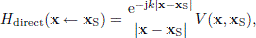$$\begin{array}{c}\hfill H_{\mathrm{direct}}(\mathbf{x}\leftarrow {\mathbf{x}}_{\mathrm{S}})=\frac{{\mathrm{e}}^{-\mathrm{j}k|\mathbf{x}-{\mathbf{x}}_{\mathrm{S}}|}}{|\mathbf{x}-{\mathbf{x}}_{\mathrm{S}}|}V(\mathbf{x},{\mathbf{x}}_{\mathrm{S}}),\end{array}$$(2)

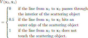
where k = ω/c is the wave number and c is the speed of sound. The function V(x₂,x₁) is a visibility function for a point pair (x₂,x₁)¹:

$$\begin{array}{cc}& V({\mathbf{x}}_2,{\mathbf{x}}_1)\hfill \\ \hfill & =\{\begin{array}{cc}0\hfill & \text{if the line from}{\mathbf{x}}_1\text{to}{\mathbf{x}}_2\text{passes through}\hfill \\ \hfill & \text{the interior of the scattering object}\hfill \\ 0.5\hfill & \text{if the line from}{\mathbf{x}}_1\text{to}{\mathbf{x}}_2\text{hits an}\hfill \\ \hfill & \text{outer edge of the scattering object}\hfill \\ 1\hfill & \text{if the line from}{\mathbf{x}}_1\text{to}{\mathbf{x}}_2\text{does not}\hfill \\ \hfill & \text{touch the scattering object}.\hfill \end{array}\hfill \end{array}$$(3)

The second transfer function in equation (1) is the specular reflection,

$$\begin{array}{c}\hfill H_{\mathrm{spec}.}(\mathbf{x}\leftarrow {\mathbf{x}}_{\mathrm{IS}})=\frac{{\mathrm{e}}^{-\mathrm{j}k|\mathbf{x}-{\mathbf{x}}_{\mathrm{IS}}|}}{|\mathbf{x}-{\mathbf{x}}_{\mathrm{IS}}|}[1-V(\mathbf{x},{\mathbf{x}}_{\mathrm{IS}})],\end{array}$$(4)

where the image source position is x_IS². The third transfer function in equation (1) is the first-order diffraction term which is a sum of contributions from the subset of the N_edges straight edges that are visible from the source and the receiver,

$$\begin{array}{cc}& H_{\mathrm{diff}.1}(\mathbf{x}\leftarrow {\mathbf{x}}_{\mathrm{S}})=-\frac{1}{4\pi }\sum _{n=1}^{N_{\mathrm{edges}}}{V}^{\prime }({\mathrm{E}}_n,\mathbf{x})V^{\prime }({\mathrm{E}}_n,{\mathbf{x}}_{\mathrm{S}}){\nu }_{{\mathrm{E}}_n}\hfill \\ \hfill & \times {\int }_{{\mathbf{x}}_{\mathrm{e}}\in {\mathrm{E}}_n}\frac{{\mathrm{e}}^{-\mathrm{j}k|\mathbf{x}-{\mathbf{x}}_{\mathrm{e}}|}}{|\mathbf{x}-{\mathbf{x}}_{\mathrm{e}}|}\frac{{\mathrm{e}}^{-\mathrm{j}k|{\mathbf{x}}_{\mathrm{e}}-{\mathbf{x}}_{\mathrm{S}}|}}{|{\mathbf{x}}_{\mathrm{e}}-{\mathbf{x}}_{\mathrm{S}}|}\beta (\mathbf{x}\leftarrow {\mathbf{x}}_{\mathrm{e}}\leftarrow {\mathbf{x}}_{\mathrm{S}})\mathrm{d}{z}_{\mathrm{e}},\hfill \end{array}$$(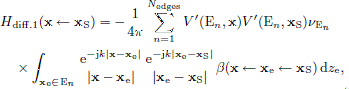5)

where V′ is a point-to-edge visibility function³:

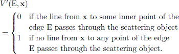$$\begin{array}{cc}& V^{\prime }(\mathrm{E},\mathbf{x})\hfill \\ \hfill & =\{\begin{array}{cc}0\hfill & \text{if the line from x to some inner point of the}\hfill \\ \hfill & \text{edge E passes through the scattering object}\hfill \\ 1\hfill & \text{if no line from x to any point of the edge}\hfill \\ \hfill & \text{E passes through the scattering object}.\hfill \end{array}\hfill \end{array}$$(6)

The integration variable, z_e, is the position along the straight edge E _n, and the function β(x ← x_e ← x_S) is an edge source directivity function which depends on the source point, x_S, the point along the edge (which is integrated over), x_e, and the receiver point, x. The directivity function β is described in several other papers and is not detailed any further here [20]. Finally, the factor ν_{E n} is the wedge index of edge E _n, defined by ν = π/θ_E, where θ_E is the wedge angle, which is 2π for a thin plate, 3π/2 for the edge of a cuboid, viewed from the outside, and θ_E = π/2 for the edge of a cuboid, viewed from the inside. Finally, the fourth transfer function in equation (1) is the sum of second- and higher-order diffraction. In the ESIE method, the edge source amplitude, q(x_e1 ← x_e2), represents the sum of second and higher-order diffraction. The edge source amplitudes are computed and subsequently propagated to the external receivers. The edge source amplitude, q(x_e1 ← x_e2), can be viewed as a directional source amplitude for an edge source at x_e2, giving the amplitude in the direction of all other edge points, x_e1, that can be seen from edge point x_e2. The edge source amplitudes are solutions to an integral equation where E_e2 denotes the edge that the point x_e2 belongs to, and ν_Ee2 is the wedge index of the same edge,

$$\begin{array}{cc}& q({\mathbf{x}}_{\mathrm{e}1}\leftarrow {\mathbf{x}}_{\mathrm{e}2})=q_0({\mathbf{x}}_{\mathrm{e}1}\leftarrow {\mathbf{x}}_{\mathrm{e}2})-\frac{{\nu }_{{\mathrm{E}}_{\mathrm{e}2}}}{8\pi }{V}^{\prime }({\mathrm{E}}_{\mathrm{e}2},{\mathbf{x}}_{\mathrm{e}1})\hfill \\ \hfill & \times \sum _{n=1}^{N_{\mathrm{edges}}}{V}^{\prime }({\mathrm{E}}_n,{\mathbf{x}}_{\mathrm{e}2}){\int }_{{\mathbf{x}}_{\mathrm{e}}\in {\mathrm{E}}_n}q({\mathbf{x}}_{\mathrm{e}2}\leftarrow {\mathbf{x}}_{\mathrm{e}})\frac{{\mathrm{e}}^{-\mathrm{j}k|{\mathbf{x}}_{\mathrm{e}2}-{\mathbf{x}}_{\mathrm{e}}|}}{|{\mathbf{x}}_{\mathrm{e}2}-{\mathbf{x}}_{\mathrm{e}}|}\hfill \\ \hfill & \times \beta ({\mathbf{x}}_{\mathrm{e}1}\leftarrow {\mathbf{x}}_{\mathrm{e}2}\leftarrow {\mathbf{x}}_{\mathrm{e}})\mathrm{d}{z}_{\mathrm{e}},\hfill \end{array}$$(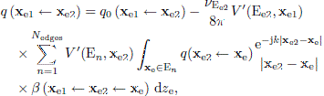7)

where the term q₀ is the contribution from the primary source,

$$\begin{array}{cc}\hfill q_0({\mathbf{x}}_{\mathrm{e}1}\leftarrow {\mathbf{x}}_{\mathrm{e}2})& =-Q_{\mathrm{S}}\frac{{\nu }_{{\mathrm{E}}_{\mathrm{e}2}}}{8\pi }{V}^{\prime }({\mathrm{E}}_{\mathrm{e}2},{\mathbf{x}}_{\mathrm{e}1})V^{\prime }({\mathrm{E}}_{\mathrm{e}2},{\mathbf{x}}_{\mathrm{S}})\hfill \\ \hfill & \times \frac{{\mathrm{e}}^{-\mathrm{j}k|{\mathbf{x}}_{\mathrm{e}2}-{\mathbf{x}}_{\mathrm{S}}|}}{|{\mathbf{x}}_{\mathrm{e}2}-{\mathbf{x}}_{\mathrm{S}}|}\beta ({\mathbf{x}}_{\mathrm{e}1}\leftarrow {\mathbf{x}}_{\mathrm{e}2}\leftarrow {\mathbf{x}}_{\mathrm{S}}).\hfill \end{array}$$(8)

The integral equation in equation (7) can be illustrated as in Figure 1a, where a single path from an edge point x_e is illustrated. Once the edge source amplitudes have been determined by finding the solution to the integral equation (7), these edge sources represent diffraction of second order and higher. The contribution to the receiver point can be computed as a sum across all edge pairs that can see each other, and the second edge in each pair can see the receiver. For each such visible edge pair, a double integral gives the higher-order diffraction contribution,

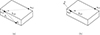Figure 1 (a) The integral equation in equation (7) expresses that the edge source amplitude at edge point xe2, in the direction of edge point xe1, is given as an integral over contributions from all edge points xe which can see xe2. (b) An additional contribution, q0(xe1 ← xe2), is caused by the primary source S.

$$\begin{array}{cc}& H_{\mathrm{HOD}}(\mathbf{x}\leftarrow {\mathbf{x}}_{\mathrm{S}})=-\frac{1}{8\pi }\sum _{n=1}^{N_{\mathrm{edges}}}{V}^{\prime }({\mathrm{E}}_n,\mathbf{x}){\nu }_{{\mathrm{E}}_n}\sum _{m=1}^{N_{\mathrm{edges}}}{V}^{″}({\mathrm{E}}_n,{\mathrm{E}}_m)\hfill \\ \hfill & \times {\int }_{{\mathbf{x}}_{\mathrm{e}1}\in {\mathrm{E}}_n}{\int }_{{\mathbf{x}}_{\mathrm{e}2}\in {\mathrm{E}}_m}q({\mathbf{x}}_{\mathrm{e}1}\leftarrow {\mathbf{x}}_{\mathrm{e}2})\frac{{\mathrm{e}}^{-\mathrm{j}k|\mathbf{x}-{\mathbf{x}}_{\mathrm{e}1}|}}{|\mathbf{x}-{\mathbf{x}}_{\mathrm{e}1}|}\hfill \\ \hfill & \times \frac{{\mathrm{e}}^{-\mathrm{j}k|{\mathbf{x}}_{\mathrm{e}1}-{\mathbf{x}}_{\mathrm{e}2}|}}{|{\mathbf{x}}_{\mathrm{e}1}-{\mathbf{x}}_{\mathrm{e}2}|}\beta (\mathbf{x}\leftarrow {\mathbf{x}}_{\mathrm{e}1}\leftarrow {\mathbf{x}}_{\mathrm{e}2})\mathrm{d}{z}_{\mathrm{e}2}\mathrm{d}{z}_{\mathrm{e}1},\hfill \end{array}$$(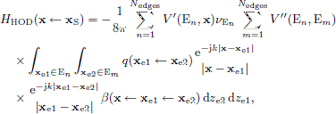9)

where V″(E₁,E₂) is an edge-to-edge visibility function: V″ = 1 if the two edges belong to the same side/face of a polygonal scattering object, and V″ = 0 if the two edges do not belong to the same side. Figure 2 illustrates a single path from one edge point, x_e2, via edge point, x_e1, to the receiver R at point x.

Figure 2 The propagation of the edge source amplitude, q(xe1 ← xe2), to the receiver point R.

2.2 Introducing secondary surface sources

If a scattering body has some part of the surface with a non-rigid boundary condition, secondary sources can be introduced to represent such an “impedance patch". A numerically simple approach is to introduce N_SS virtual pistons centered at locations x_SS,i, and then let these secondary source pistons get a vibration amplitude u_SS,i which, together with the field from a primary sound source for a rigid scattering object, generates a field which fulfills the boundary condition at the impedance patch. Exactly how the boundary condition is formulated mathematically will determine how the secondary source amplitudes should be derived. Once the vibration velocities of the secondary source pistons have been determined, the sound radiated from these pistons can be computed with the ESIE method, that is, for the boundary condition of a rigid scattering body. This can be illustrated as in Figure 3 and formulated as

Figure 3 The secondary source approach in equation (10) adds (a) the sound field generated by the primary source S and the rigid scattering object, and (b) the sound fields radiated by secondary piston sources SSi with vibration velocities uSS,i, when pistons are set in a rigid scattering object. Only the geometrical acoustics components are illustrated; diffraction components should be added to both (a) and (b).

$$\begin{array}{c}\hfill p_{\mathrm{total}}(\mathbf{x})=Q_{\mathrm{S}}H(\mathbf{x}\leftarrow {\mathbf{x}}_{\mathrm{S}})+\sum _{i=1}^{N_{\mathrm{SS}}}{u}_{\mathrm{SS},i}G(\mathbf{x}\leftarrow {\mathbf{x}}_{{\mathrm{SS}}_i}),\end{array}$$(10)

where G(x ← x_{SS i}) is the transfer function from piston source number i to the sound pressure at location x, with the vibration velocity u_{SS i} being the source signal instead of the Q_S used for the point-to-point H transfer functions. It can be noted that the G transfer functions should also fulfil the rigid boundary condition of the scattering object and thus, the same decomposition as in equation (1) can be used. The piston velocities, u_SS,i, are found by storing the N_SS unknown, to be determined, values in a vertical array, u_SS, and formulating a matrix equation,

$$\begin{array}{c}\hfill [{\mathbf{G}}_{\mathrm{front}}+{\mathbf{G}}_{\mathrm{rear}}]{\mathbf{u}}_{\mathrm{SS}}={\mathbf{p}}_{\mathrm{excitation}},\end{array}$$(11)

where p_excitation is a vertical array of the sound pressure amplitudes caused by the primary source at the secondary source pistons’ central points with a rigid boundary condition at the piston locations,

$$\begin{array}{c}\hfill {\mathbf{p}}_{\mathrm{excitation}}=\left[p_{\mathrm{excitation}}({\mathbf{x}}_i)\right]=Q_{\mathrm{S}}[H({\mathbf{x}}_{\mathrm{SS},i}\leftarrow {\mathbf{x}}_{\mathrm{S}})].\end{array}$$(12)

The values in u_SS can then apparantly be found via a matrix inversion,

$$\begin{array}{c}\hfill {\mathbf{u}}_{\mathrm{SS}}={[{\mathbf{G}}_{\mathrm{front}}+{\mathbf{G}}_{\mathrm{rear}}]}^{-1}{\mathbf{p}}_{\mathrm{excitation}},\end{array}$$(13)

where it is assumed that this inversion exists and can be computed. Inspecting the matrices involved, G_front is a square matrix of the transfer functions, G(x ← x_{SS i}) like in equation (10), from all the N_SS secondary source pistons to the N_SS receiver positions at the center of the secondary source pistons:

$$\begin{array}{cc}\hfill {\mathbf{G}}_{\mathrm{front}}& =\left[G_{\mathrm{front},ij}\right]\hfill \\ \hfill & =\left[G_{\text{front, SS mid-point}i\leftarrow \text{SS piston}j}\right].\hfill \end{array}$$(14)

The second matrix in equation (11), G_rear, describes the transfer functions into the impedance surface. Two different models of impedance materials lead to different matrix structures. For a locally reacting impedance material model, there is no cross-coupling between the secondary source pistons on the rear side, so for a locally reacting impedance material,

$$\begin{array}{c}\hfill {\mathbf{G}}_{\mathrm{rear}}=Z_{\mathrm{s},\mathrm{target}}\mathbf{I},\end{array}$$(15)

where I is the identity matrix of size (N_SS,N_SS) and Z_s,target is the intended/target impedance value. The impedance should be the specific acoustic impedance, that is, Z_s = p/u where u is the normal particle velocity at the surface of the impedance material. This target value could have different values for each secondary source i, and then G_rear would have different values along the diagonal of the matrix. On the other hand, for an extended reaction impedance material model, the matrix G_rear will be full with values of cross-transfer functions:

$$\begin{array}{cc}\hfill {\mathbf{G}}_{\mathrm{rear}}& =\left[G_{\mathrm{rear},ij}\right]\hfill \\ \hfill & =\left[G_{\text{rear, SS mid-point}i\leftarrow \text{SS piston}j}\right].\hfill \end{array}$$(16)

These individual transfer functions, G_rear,-pagination _{SS mid-point i ← SS piston j}, should be computed with a realistic model of the impedance material and all other SS pistons than j having a rigid BC.

3 Computational aspects

For the four H-transfer functions in equation (1), computational aspects have been described in previous publications, for 3D-geometries. The first-order diffraction integral is described in [20, 21], and the integral equation solving with the Nyström method (gaussian quadrature) is described in [6]. For the numerical example in Section 4, H-transfer functions for 2D cases must be computed which requires somewhat modified expressions as described in Section 3.1 below. Furthermore Section 3.2 describes the computation of the piston-to-point G-transfer functions in the ESIE+SS context.

3.1 Point-to-point transfer functions, H^2D, in 2D

The 2D transfer functions will be denoted H^2D below, and they will have to use a modified source signal, Q′_S, such that

$$\begin{array}{c}\hfill p^{2\mathrm{D}}(\mathbf{x})=Q_{\mathrm{S}}^{\prime }{H}^{2\mathrm{D}}(\mathbf{x}\leftarrow {\mathbf{x}}_{\mathrm{S}}),\end{array}$$(17)

where Q′_S = U′_Sωρ₀/4 and U′_S is the volume velocity per unit length of the line source (with the dimension m²/s).

3.1.1 The direct sound and the specular reflection

The direct sound, and specular reflection, transfer functions are given by the Hankel function of first kind and order 0 [1],

$$\begin{array}{c}\hfill \{\begin{array}{c}{H}_{\mathrm{direct}}^{2\mathrm{D}}(\mathbf{x}\leftarrow {\mathbf{x}}_{\mathrm{S}})={\mathrm{H}}_0(k|\mathbf{x}-{\mathbf{x}}_{\mathrm{S}}|)V(\mathbf{x},{\mathbf{x}}_{\mathrm{S}})\hfill \\ H_{\mathrm{spec}.}^{2\mathrm{D}}(\mathbf{x}\leftarrow {\mathbf{x}}_{\mathrm{IS}})={\mathrm{H}}_0(k|\mathbf{x}-{\mathbf{x}}_{\mathrm{IS}}|)(1-V(\mathbf{x},{\mathbf{x}}_{\mathrm{IS}})).\hfill \end{array}\end{array}$$(18)

These two GA components are also subject to visibility tests via the V-functions.

3.1.2 First-order diffraction

The first-order diffraction term can be computed using the expression given in [1]. Thus, for a source with polar coordinates x_S = (R_S,θ_S) and a receiver at x = (R_R,θ_R), a wedge with sides at θ = 0 and θ = θ_W = π/ν, R_< denoting the smaller of [R_S,R_R], and R_> denoting the larger of [R_S,R_R],

$$\begin{array}{cc}& H_{\mathrm{diff}.1}^{2\mathrm{D}}(\mathbf{x}\leftarrow {\mathbf{x}}_{\mathrm{S}})=2\nu \sum _{n=0}^{\infty }{ϵ}_{n}cos(n\nu {\theta }_{\mathrm{R}})cos(n\nu {\theta }_{\mathrm{S}})\hfill \\ \hfill & \times {\mathrm{H}}_{n\nu }(k{R}_{>}){\mathrm{J}}_{n\nu }(k{R}_{<})-V_{\text{single wedge}}(\mathbf{x},{\mathbf{x}}_{\mathrm{S}})\hfill \\ \hfill & \times {\mathrm{H}}_0(k|\mathbf{x}-{\mathbf{x}}_{\mathrm{S}}|)-[1-V_{\text{single wedge}}(\mathbf{x},{\mathbf{x}}_{\mathrm{IS}})]\hfill \\ \hfill & \times {\mathrm{H}}_0(k|\mathbf{x}-{\mathbf{x}}_{\mathrm{IS}}|),\hfill \end{array}$$(19)

where ϵ₀ = 1 and ϵ _n = 2,n ≠ 0, and J _nν,H _nν are, respectively, the Bessel and Hankel functions of first kind and order nν. In this expression, the approach from [22] is used: the sum in equation (19) contains also the potential direct sound and specular reflection, so in order to get the diffracted field only, the direct sound and specular reflection must be subtracted – but only if they are visible according to the same GA principles as above. The notation V_{single wedge}(x,x_S) should be understood such that the visibility is tested for an imagined single edge with semi-infinite wedge faces.

In the special case that the source and receiver are in the same position, then the sum in equation (19) diverges and some extra steps must be taken to subtract the singular direct sound term, as described in [22], but that special case is left out here. Even if the source and receiver are not in the same location, the closer R_< and R_> are to each other, the slower the sum in equation (19) converges. In addition, for high-order terms, the Hankel and the Bessel functions get, respectively, extremely large and small values. Thus, for high-order terms, the asymptotic formulas, valid when the order is much larger than the argument, need to be used. The product of the Hankel function and the Bessel function is, if nν ≫ kR [23],

$$\begin{array}{cc}& H_{n\nu }(k{R}_{>})·J_{n\nu }(k{R}_{<})\hfill \\ \hfill & =[J_{n\nu }(k{R}_{>})-\mathrm{j}{Y}_{n\nu }(k{R}_{>})]J_{n\nu }(k{R}_{<})\hfill \\ \hfill & \sim -\mathrm{j}{Y}_{n\nu }(k{R}_{>})J_{n\nu }(k{R}_{<})\hfill \\ \hfill & \sim \mathrm{j}\sqrt{\frac{2}{\pi n\nu }}{\left(\frac{\mathrm{e}k{R}_{>}}{2n\nu }\right)}^{-n\nu }\frac{1}{\sqrt{2\pi n\nu }}{\left(\frac{\mathrm{e}k{R}_{<}}{2n\nu }\right)}^{n\nu }\hfill \\ \hfill & =\frac{\mathrm{j}}{\pi n\nu }{\left(\frac{R_{<}}{R_{>}}\right)}^{n\nu },\hfill \end{array}$$(20)

and higher-order terms are then straightforward to compute.

3.1.3 Higher-order diffraction

For the higher-order diffraction, the explicit line source expression in equation (18) can not be used since the ESIE method requires monopole sources. Instead, the line source has to be implemented as a distribution of monopoles, using the integral relationship for the Hankel function, where symmetry permits halving the integration range:

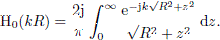$$\begin{array}{c}\hfill {\mathrm{H}}_0(kR)=\frac{2\mathrm{j}}{\pi }{\int }_0^{\infty }\frac{{\mathrm{e}}^{-\mathrm{j}k\sqrt{R^2+z^2}}}{\sqrt{R^2+z^2}}\mathrm{d}z.\end{array}$$(21)

This integral can be approximated by a set of monopoles distributed over a finite length, which represents a truncated version of the infinite integral. Thus, for a finite length of L meters, with N_monopoles distributed from 0 to L/2,

$$\begin{array}{cc}\hfill {\mathrm{H}}_0(kR)& \approx \frac{2\mathrm{j}}{\pi }{\int }_0^{L/2}\frac{{\mathrm{e}}^{-\mathrm{j}k\sqrt{R^2+z^2}}}{\sqrt{R^2+z^2}}\mathrm{d}z\hfill \\ \hfill & \approx \frac{\mathrm{j}\mathrm{\Delta }z}{\pi }[\frac{{\mathrm{e}}^{-\mathrm{j}kR}}{R}+2\sum _{n=2}^{N_{\mathrm{monopoles}}}\frac{{\mathrm{e}}^{-\mathrm{j}k\sqrt{R^2+z_n^2}}}{\sqrt{R^2+z_n^2}}],\hfill \end{array}$$(22)

where z_n = (n − 1)Δz and Δz = L/[2(N_monopoles − 1)]. The truncation will give interference effects which can be reduced with a tapering of the source amplitude, e.g. with a raised cosine window such that

$$\begin{array}{cc}\hfill {\mathrm{H}}_0(kR)& \approx \frac{\mathrm{j}\mathrm{\Delta }z}{\pi }[\frac{{\mathrm{e}}^{-\mathrm{j}kR}}{R}+2\sum _{n=2}^{N_{\mathrm{monopoles}}}\frac{{\mathrm{e}}^{-\mathrm{j}k\sqrt{R^2+z_n^2}}}{\sqrt{R^2+z_n^2}}\frac{1}{2}\hfill \\ \hfill & \times (1-cos\frac{\pi (n+N_{\mathrm{monopoles}}-1)}{N_{\mathrm{monopoles}}})].\hfill \end{array}$$(23)

The expression in equation (23) implies that a diffraction 2D transfer function, of first or higher order, $H_{\mathrm{diff}.1}^{2\mathrm{D}}/H_{\mathrm{HOD}}^{2\mathrm{D}}$, can be computed with the ESIE method by summing the contributions by a set of N_monopoles monopoles placed at z-coordinates z_n. Since the ESIE method will give 3D H transfer functions, the scaling is, as implied by equation (23),

$$\begin{array}{cc}& \left\{\begin{array}{c}{H}_{\mathrm{diff}.1}^{2\mathrm{D}}\\ [4pt]H_{\mathrm{HOD}}^{2\mathrm{D}}\end{array}\right\}=\frac{\mathrm{j}\mathrm{\Delta }z}{\pi }[\left\{\begin{array}{c}{H}_{\mathrm{diff}.1,n=1}^{3\mathrm{D}}\\ [4pt]H_{\mathrm{HOD},n=1}^{3\mathrm{D}}\end{array}\right\}+2\sum _{n=2}^{N_{\mathrm{monopoles}}}\hfill \\ \hfill & \times \left\{\begin{array}{c}{H}_{\mathrm{diff}.1,n}^{3\mathrm{D}}\\ [4pt]H_{\mathrm{HOD},n}^{3\mathrm{D}}\end{array}\right\}\frac{1}{2}(1-cos\frac{\pi (n+N_{\mathrm{monopoles}}-1)}{N_{\mathrm{monopoles}}})].\hfill \end{array}$$(24)

To demonstrate the accuracy, a first-order diffraction transfer function is computed with equation (19) as reference result and $H_{\mathrm{diff}.1}^{2\mathrm{D}}$ computed as a sum of 501 monopoles using equation (24). An arbitrarily chosen wedge geometry was chosen, with r_S = 1 m, r_R = 0.5 m, θ_S = π/4, θ_R = π/2, θ_W = 3π/2, and the results are shown in Figure 4. As is clear from Figure 4b the monopole source amplitude tapering reduces the error substantially.

Figure 4 First-order diffraction TF in 2D computed with the ref. expression, equation (19), and via a set of monopoles, equation (24), with and without source amplitude tapering. (a) The three TFs. (b) The error for the two monopole distributions.

3.2 Piston-to-point transfer functions, G

3.2.1 The direct sound and the specular reflection

For a piston sound source, the sum of the direct sound and the specular reflection is given by the Rayleigh integral, which should be evaluated across the piston, denoted by P below, so

$$\begin{array}{cc}& G_{\mathrm{direct}}(\mathbf{x}\leftarrow {\mathbf{x}}_{\mathrm{S}})+G_{\mathrm{spec}.}(\mathbf{x}\leftarrow {\mathbf{x}}_{\mathrm{S}})\hfill \\ \hfill & =\frac{\mathrm{j}\omega {\rho }_0}{2\pi }\int {\int }_{{\mathbf{x}}_{\mathrm{S}}\in \mathrm{P}}\frac{{\mathrm{e}}^{-\mathrm{j}kr}}{r}\mathrm{d}{x}_{\mathrm{S}}\mathrm{d}{y}_{\mathrm{S}},\hfill \end{array}$$(25)

where r = |x ← x_S|. Various equivalent representations are available for the numerical computation of the Rayleigh integral [24]. A plane-wave + piston edge-wave formulation can be derived from the time-domain version in [25], leading to

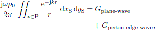$$\begin{array}{cc}\hfill \frac{\mathrm{j}\omega {\rho }_0}{2\pi }\int {\int }_{\mathbf{x}\in \mathrm{P}}\frac{{\mathrm{e}}^{-\mathrm{j}kr}}{r}\mathrm{d}{x}_{\mathrm{S}}\mathrm{d}{y}_{\mathrm{S}}& =G_{\text{plane-wave}}\hfill \\ \hfill & +G_{\text{piston edge-wave}},\hfill \end{array}$$(26)

where the location of the perpendicular projection of the receiver point onto the baffle, denoted x_proj., and the height h of the receiver point above the baffle, see Figure 5a, determine the plane-wave term:

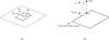Figure 5 Geometrical parameters for the plane-wave + piston edge-wave model. (a) The plane wave component exists if the projection, xproj., onto the baffle of a receiver position, x, falls inside the piston, as is the case for position x1 but not for x2. (b) The edge wave uses a local spherical coordinate system, (r,θ,φ), for each position, xe, along the piston edges.

$$\begin{array}{cc}& G_{\text{plane-wave}}={\rho }_{0}c{\mathrm{e}}^{-\mathrm{j}kh}\hfill \\ \hfill & \times \{\begin{array}{cc}0\hfill & \text{if}{\mathbf{x}}_{\mathrm{proj}.}\text{is outside the piston}\hfill \\ 0.5\hfill & \text{if}{\mathbf{x}}_{\mathrm{proj}.}\text{is exactly on an edge of the piston}\hfill \\ 1\hfill & \text{if}{\mathbf{x}}_{\mathrm{proj}.}\text{is inside the piston},\hfill \end{array}\hfill \end{array}$$(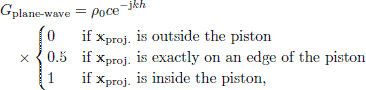27)

and the piston edge-wave term is a sum of integral contributions from the N_PE piston edges⁴,

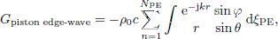$$\begin{array}{c}\hfill G_{\text{piston edge-wave}}=-{\rho }_{0}c\sum _{n=1}^{N_{\mathrm{PE}}}\int \frac{{\mathrm{e}}^{-\mathrm{j}kr}}{r}\frac{sin\phi }{sin\theta }\mathrm{d}{\xi }_{\mathrm{PE}},\end{array}$$(28)

where the angles (θ,φ) describe the direction of the receiver point, expressed in a spherical coordinate system which is local to the piston edge point, ξ_PE, see Figure 5b. The angle θ is the angle from the local z-axis = the piston plane normal vector. Thus, for receivers in the same plane as the piston, θ = π/2 and for a receiver exactly above one particular piston edge point, θ = 0. Furthermore, the angle φ is the angle in the plane of the baffle between two vectors: one being the local piston edge tangent = the ξ_PE-axis and the other the vector from the piston edge point to the receiver projection point x_proj.. The plane-wave + piston edge-wave formulation makes it straightforward to compute the transfer function for receivers arbitrarily close to the piston surface. Only for receivers very close to an edge of a piston will the 1/r-singularity cause numerical challenges. This is in contrast to a direct computation of the Rayleigh integral where any receiver point at the piston surface requires special handling of the 1/r-singularity.

The 2D-case corresponds to a “line piston”, meaning a strip-like piston of infinite extension in one direction, and the edge waves of two parallel edges must be computed. The infinite extension of these piston edges leads to a computationally expensive oscillating integral in equation (28), which could be computed efficiently by deriving the numerical method of steepest descent for this case [21]. Here, however, the time-domain integral for a long but finite piston is chosen, followed by an FFT and interpolation to a desired frequency value. The plane-wave + piston edge-wave formulation in [25] was presented as an impulse response formulation, which is cheap to compute because of the non-oscillating impulse response character. For a discrete-time impulse response, the plane-wave becomes a pulse of amplitude ρ₀c at the first IR sample (time zero), when the receiver is immediately at the center of the piston, that is, for G_{SSi ← SSi}. For other combinations of SSi ← SSj,i ≠ j, no plane wave components exists. If a receiver position is at a distance from the piston, but with x_proj. inside the piston, the pulse should be delayed by the number of samples, n_delay = hf_S/c but this delay value will typically be a non-integer. Some technique for fractional delays [26], could be employed for that situation.

The line piston generates two edge waves, and for a discrete-time impulse response, g(t _n), each edge generates an impulse response where each sample’s value is [25],

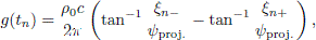$$\begin{array}{c}\hfill g(t_n)=\frac{{\rho }_{0}c}{2\pi }({tan}^{-1}\frac{{\xi }_{n-}}{{\psi }_{\mathrm{proj}.}}-{tan}^{-1}\frac{{\xi }_{n+}}{{\psi }_{\mathrm{proj}.}}),\end{array}$$(29)

where ξ _n± are the two endpoints along an edge segment which contribute to the impulse response within the time period t _n ± Δt/2 = (n ± 0.5)/f_S) where f_S is the sampling frequency. The parameter ψ_proj. is the perpendicular (shortest) distance from the edge to the projection of the receiver point onto the baffle. The sign of ψ_proj. determines the polarity of the edge wave, and Figure 6 illustrates the definition of the ξ- and ψ_proj.-parameters, for the edge in question, as well as for the second edge, ξ′ and ψ′_proj.. It can be noted that for a receiver point the projection point of which falls outside the piston, the ψ parameter will have opposite signs for the two piston edge contributions whereas they will both be positive when the projection point falls inside the piston. In Figure 6 the two distances are

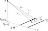Figure 6 Geometrical parameters for the edge-wave impulse response calculation for a line piston. The coordinates (ξ′,ψ′) are indicated for the calculation of the second edge’s contribution.

$$\begin{array}{c}\hfill \{\begin{array}{c}{r}_{n-}=c(t_n-\frac{\mathrm{\Delta }t}{2})=\frac{c(n-0.5)}{f_{\mathrm{S}}}=\sqrt{{\xi }_{n-}^2+{\psi }_{\mathrm{proj}.}^2+h^2}\hfill \\ r_{n+}=c(t_n+\frac{\mathrm{\Delta }t}{2})=\frac{c(n-0.5)}{f_{\mathrm{S}}}=\sqrt{{\xi }_{n+}^2+{\psi }_{\mathrm{proj}.}^2+h^2}.\hfill \end{array}\end{array}$$(30)

For each n, these square root expressions can give the values of ξ_n±².

3.2.2 First- and higher-order diffraction

For the first- and higher-order diffraction, the piston source can be approximated with a set of monopoles distributed across the piston surface, both for the 2D and 3D cases. The first-order diffraction from a line/strip piston could be computed as described in Section 3.2.1 by representing the strip piston with a line source at the center of the piston. However, G transfer functions must be computed for receivers directly at the piston surface, and then the approach to subtract the direct sound as in equation (19) requires the special steps described in [22]. Here, instead, the line piston is represented by a set of monopoles for a piston of finite length since the first-order diffraction can be computed explicitly for a monopole. Also for higher-order diffraction, the line piston is represented by a set of monopoles as described in Section 3.1.3.

3.3 Computational load

The computational load involved in these steps can be summarized through an example with a single primary source, n_receiver receiver positions/fieldpoints, and an impedance patch which is discretized with N_SS secondary source pistons. Then a number of transfer functions needs to be computed, all with a rigid boundary condition for all of the scattering object:

− n_receiver + N_SS point-to-point transfer functions, H.

− n_receiver(n_receiver + N_SS) piston-to-point transfer functions, G.

If an extended-reaction impedance material model is intended, then an additional set of N_SS ⋅ N_SS piston-to-point transfer functions must be computed. This secondary source approach will be efficient when the value N_SS is low, that is, when scattering objects are mostly rigid but with some non-rigid parts. As the value N_SS is increased, both the computation of G transfer functions and the related matrix inversion will quickly get very costly. However, as discussed later the N_SS ⋅ N_SS piston-to-centre-of-piston G transfer functions might be approximated well if the diffraction terms are left out. The computation of such transfer functions is cheap when only GA components are included since such a case represents the classical case of a piston in an infinite baffle.

4 Numerical example

4.1 Studied case

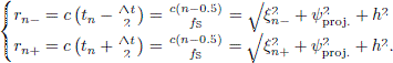
A rigid box was modeled numerically in 2D with dimensions as shown in Figure 7, which also shows the location of a 2D point source (= a 3D line source) S, and two sets of receivers, R: an “external" circle of receivers, in Figure 7a, and a set of nearfield receivers, in Figure 7b. In the nearfield set two parallel lines of receivers are placed at 1 cm and 2 cm distance from the surface of the box, respectively, facilitating a study of the sound pressure as well as the particle velocity (approximated from the sound pressure difference) and the impedance, with Δx = 1 cm:

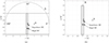Figure 7 Geometrical details for the numerical example with a mostly rigid box, sized 3 m by 0.2 m, and a small patch with a locally reacting impedance boundary condition. A 2D point source is marked S. In (a), a semicircle of external receivers are placed at a radius of 3.1 m, with an angle step of 1 degree (not all are shown). In (b), two rows of receivers are placed at 1 cm and 2 cm distance (in the x-direction) from the box surface, in steps of 2 cm in the y-direction (not all are shown). An initial test case used an all-rigid box, without the impedance patch. The numerically most challenging receiver directions are marked with darker grey areas, and the more benign challenging directions are marked with lighter grey areas.

$$\begin{array}{c}\hfill \{\begin{array}{c}{v}_x(x=1.5\mathrm{cm})\approx -[p(x=2\mathrm{cm})-p(x=1\mathrm{cm})]\hfill \\ /\left(\mathrm{j}\omega {\rho }_0\mathrm{\Delta }x\right)\hfill \\ p(x=1.5\mathrm{cm})\approx \frac{1}{2}[p(x=2\mathrm{cm})+p(x=1\mathrm{cm})]\hfill \\ Z_{s,x}(x=1.5\mathrm{cm})=p(x=1.5\mathrm{cm})/v_x(x=1.5\mathrm{cm}).\hfill \end{array}\end{array}$$(31)

The circle of receivers is placed at a radius of 3.1 m from the origin = the center of the box. A 30 cm wide strip of an absorbing material is positioned at the source side of the scattering box. This small impedance patch size was chosen to keep the ESIE+SS calculations moderate. As an initial test, an all-rigid version of the box was studied without any impedance strip. The values chosen for the impedance are given in the , and they represent a porous material with a flow resisitivity of 10 kPa s/m² and 20 cm thickness against a rigid backing. Mechel’s model was used for the modeling, as implemented in the modeling software “Norflag" [27]. Calculations were done for the 18 third-octave band center frequencies from 50 Hz to 2.5 kHz,

$$\begin{array}{c}\hfill f_n=1000\times {10}^{n/10}\mathrm{Hz},n\in [-13,4].\end{array}$$(32)

In tables and figures, the frequency labels 50 Hz, 63 Hz, 80 Hz etc will be used, rather than the accurate frequency values 50.12 Hz, 63.10 Hz, 79.43 Hz etc.

4.2 Numerical details for the FEM calculations

For the FEM modeling, COMSOL Multiphysics, v 6.1, with the Acoustics module was used and the geometry of the model used is shown in Figure 8. The “pressure acoustics" domain indicated in Figure 8 was meshed with triangular elements with a maximum element side length of 6.88 mm. The perfectly matched layer, PML, had a thickness of 5 elements in the radial direction.

Figure 8 The FEM used a 2D mesh of the area marked with grey in the figure.

4.3 Numerical details for the ESIE+SS method

The freely available Matlab “EDtoolbox" [28] was used as a basis for the secondary source method. Some extra expressions had to be implemented and Table 1 shows how the various components were computed.

Furthermore, various numerical settings were used for different frequencies, as summarized in Table 2. Very high quadrature orders were used, since the 3D-implementation of the 2D-case required quite long finite edges, which in turn lead to integrands with more and more oscillations over the integration range, as frequency increased. The use of very high quadrature orders requires high numerical precision in the calculations, and corresponding accuracy of the quadrature weights and nodes. Matlab’s standard precision (double floating point precision) has been used, and the function lgwt.m from Matlab File Exchange for generating the quadrature weights and nodes, and no problems with convergence have been observed that could be attributed to the numerical precision. A more important numerical challenge is the character of the integrand in the diffraction integrals since the integrand has strong singularities for certain source-receiver combinations. The ESIE+SS calculations involve two steps, which have quite different effects on this latter aspect: the character of the diffraction integral. These two steps are:

• 1

  In the first step, the secondary source amplitudes are calculated, and this step involves the calculation of three quantities, as seen in equation (13):

  • G_front contains 2D-piston-to-point transfer functions, which involve diffraction calculations. These diffraction calculations are well-behaved since no visibility zone boundary is close: both the source piston and the receiver point belong to the same plane (i.e., both are inside the same polygon of the polyhedral scattering object). If a source piston and receiver point are both very close to an edge, then an integrand singularity could cause numerical challenges, but the shown case doesn’t have any pistons close to an edge.

  • G_rear No diffraction is involved in these transfer functions since they represent the absorption material.

  • G_excitation contains external-source-to-point transfer functions, which involve diffraction calculations. Also these diffraction calculations are well-behaved since the original source has been positioned such that it is not aligned with any plane of the polyhedral scattering object. The numerical challenges for cases where the source is aligned with one of the scattering object planes was addressed in [xx].

• 2

  Once the secondary source amplitudes have been computed, their contributions to the external receiver points, the field points, are computed with equation (10). Here, the diffraction calculation in G(x ← x_SSi) will indeed cause numerical challenges for certain receiver positions, as illustrated in Figure 7. It is assumed that the numerical challenges will primarily be caused by the singular character of the integrand and not by the numerical precision of the quadrature per se.

The direct sound transfer functions from a piston to a center point at the same piston or another piston, G^2D(x_SS,i ← x_SS,j), were computed via impulse responses (IR) for a long strip piston as described in Section 3.2.1. A sampling frequency of 5 ⋅ 10⁶ Hz was used, 1s long impulse responses were computed, and an fft size of 2²³ gave discrete Fourier transform values from which the TF values for the desired frequencies were found via interpolation.

5 Results

5.1 Scattering from an all-rigid box to a circle of receivers

As a first case the all-rigid box was studied, computing the sound pressure with the ESIE method and the FEM for the semi-circle of receivers, shown in Figure 7a. Figures 9a–9f show the results for six example frequencies, and the typical challenge with the ESIE method is clear: for certain receiver positions, the HOD-term requires very high gaussian quadrature orders and the accuracy suffers [7]. Those challenging directions are marked with darker grey areas in Figures 7a and 9a–9f for the most challenging directions, and lighter grey areas for the slightly less challenging directions⁵. In other directions, the agreement is excellent, and Figure 10a shows the median, across the 181 receiver positions, 95% and 5% percentiles for the level difference between the ESIE results and the FEM results. For most frequencies, 90% of the values are thus within ±0.2 dB of the reference FEM results. It can be noted that the computed SPL values have a dynamic range of up to 40 dB. The ESIE results are expected to converge towards the FEM results if the Gaussian quadrature order is increased. However, the quadrature orders used to represent the 2D case are very high, as shown in Table 2, and discussed in Section 4.3.

Figure 9 Results for the scattering to the circle of receivers in Figure 7a for the all-rigid version of the box, for six example frequencies. Settings for the ESIE method were as in Table 2. The numerically most challenging receiver positions are marked with darker grey areas, and the more benign challenging positions are marked with lighter grey areas. (a) f = 50 Hz. (b) f = 125 Hz. (c) f = 250 Hz. (d) f = 500 Hz. (e) f = 1000 Hz. (f) f = 2000 Hz.

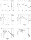Figure 10 Median-quantile-values for the calculation error for (a) the all-rigid box, calculated with the ESIE method only, and (b) the box with an impedance patch, calculated with the ESIE+SS method. In both diagrams, the quantile values are given for 18 frequencies, including those not shown in Figures 9 and 11. The median and quantile values were based on the 181 receiver angle values shown in Figures 9 and 11. In (c) results for all frequencies and all 181 receiver positions were pooled into one dataset. Note the different scale in (c).

The results presented here are considered as accurate enough to show the possibilities with the ESIE+SS method.

5.2 Scattering from the box with an impedance patch to a circle of receivers

For the main test case, the impedance patch was introduced and the ESIE method was complemented with secondary sources (SS). Thus, Figures 11a–11f show the results for the same six example frequencies as in Figure 9, for the ESIE+SS method and the FEM. The sound pressure values are very similar to those for the all-rigid box in Figures 9a–9f since the impedance patch is such a small part of the box, but distinct differences can be observed. Figure 10b shows the median, across the 181 receiver positions, 95% and 5% percentiles for the level difference between the ESIE+SS results and the FEM results.

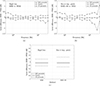Figure 11 Results for the scattering to the circle of receivers in Figure 7b for the box with an impedance patch in Figure 7b, for six example frequencies. Settings for the ESIE+SS method were as in Table 2. The numerically most challenging receiver positions are marked with solid-line arrows, and the more benign challenging positions are marked with dotted-line arrows. (a) f = 50 Hz. (b) f = 125 Hz. (c) f = 250 Hz. (d) f = 500 Hz. (e) f = 1000 Hz. (f) f = 2000 Hz.

Figure 10c compiles the two sets of data points into median+percentiles values, based on all receivers positions and frequencies. The percentile values imply that 90% of the 18 ⋅ 181 = 3258 data points have an error within [ − 0.20,+0.15] dB for the all-rigid box and [ − 0.30,+0.32] dB for the box with the impedance patch. While the error with the ESIE+SS method is larger than for the ESIE method and the all-rigid box, the accuracy must still be viewed as very good considering the dynamic range of up to 40 dB and the frequency range from 50 Hz to 2.5 kHz. Since the ESIE+SS method adds two terms, both of which are computed with the ESIE method, it is to be expected that the ESIE+SS would have a somewhat larger error than the ESIE method for a rigid box. The slightly increasing error for the highest frequencies, as seen in Figure 10b might indicate that the number of secondary sources could need to be higher than 11, as seen in Table 2. For the highest frequency, 11 secondary sources corresponds to 5 elements per wavelength at 2.5 kHz, and the simple piston elements could probably not be expected to perform any better than the results found here.

5.3 Scattering from the box with an impedance patch to near-field receivers

As shown in Figure 7b, a second set of receiver positions was placed very close to the surface of the box. Thus both the nearfield sound pressure, the nearfield particle velocity, and the specific acoustic impedance could be computed as given by equation (31). The latter should be very close to the specified locally reacting impedance value, “Target impedance”, but as the frequency increases one would expect gradually deviating values since the impedance in the sound field is computed at a short distance, 1.5 cm, from the impedance surface. The FEM software could output particle velocity values in receiver points, but here, the approximated values from the pressure differences were used instead since these should be closer to the ones computed by the ESIE method (which in its present implementation in the ED toolbox can only compute sound pressure values).

Figures 12 and 13 show the sound pressure, the particle velocity and the specific acoustic impedance for the same six frequencies as in Figures 9 and 11. Again, numerical challenges for the HOD-terms give large errors for y ⪆ 1.5 m.

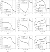Figure 12 Results for the nearfield receivers in Figure 7b for the box with an impedance patch in Figure 7a, for three example frequencies: 50 Hz, 125 Hz and 250 Hz. Subfigures (a), (d), (g) show the sound pressure level, for an arbitrary source amplitude; (b), (e), (h) show the particle velocity, expressed in dB, whereas (c), (f), (i) show the specific acoustic impedance values. Settings for the ESIE+SS method were as in Table 2. Note the different scales between plots. (a) Lp,f = 50 Hz. (b) Lv,f = 50 Hz. (c) Zs,f = 50 Hz. (d) Lp,f = 125 Hz. (e) Lv,f = 125 Hz. (f) Zs,f = 125 Hz. (g) Lp,f = 250 Hz. (h) Lv,f = 250 Hz. (i) Zs,f = 250 Hz.

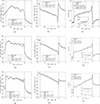Figure 13 Results for the nearfield receivers in Figure 7b for the box with an impedance patch in Figure 7a, for three example frequencies: 500 Hz, 1 kHz and 1.6 kHz. Subfigures (a), (d), (g) show the sound pressure level, for an arbitrary source amplitude; (b), (e), (h) show the particle velocity, expressed in dB, whereas (c), (f), (i) show the specific acoustic impedance values. Settings for the ESIE+SS method were as in Table 2. Note the different scales between plots. (a) Lp,f = 500 Hz. (b) Lv,f = 500 Hz. (c) Zs,f = 500 Hz. (d) Lp,f = 1 kHz. (e) Lv,f = 1 kHz. (f) Zs,f = 1 kHz. (g) Lp,f = 2 kHz. (h) Lv,f = 2 kHz. (i) Zs,f = 2 kHz.

5.4 The G transfer functions

A substantial part of the computational load for this ESIE+SS method consists of computing the G piston-to-point transfer functions for the N_SS ⋅ N_SS combinations of secondary sources in the G_front matrix. Therefore, it is relevant to investigate how large impact the inclusion of first- and higher-order diffraction has for these transfer functions. As can be seen in equation (13), the determination of the secondary source amplitudes will involve the sum of the two impedances that each secondary source experiences: the front (outside) and the rear (into the impedance material). Thus, the impact of a small error in the computation of G_front will be reduced by the addition of G_rear, which is known explicitly. One can expect that the inclusion of diffraction components in G_front would be more important for lower frequencies since diffraction waves are stronger for lower frequencies. However, the magnitude of G_front is generally increasing with frequency, since we use a piston secondary source model⁶. At the same time, for impedance materials, the values in G_rear are typically decreasing for increasing frequencies (it is difficult to get high absorption for low frequencies ↔ the impedance is high at low frequencies). So, rather fortunately, we could expect that the effect of including diffraction waves in G_front might be small across frequencies. The effect can be demonstrated through some different results. For the numerical example above, two secondary sources were used for the frequency range 50 Hz–400 Hz (see Tab. 2). For this frequency range, the magnitudes of G_{front,1 ← 1} and G_{rear,1 ← 1} are plotted in Figure 14a and a large magnitude difference can be observed, and the difference decreases rapidly as the frequency increases.

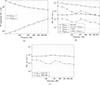Figure 14 For the numerical example in Figures 7–13, in the frequency range which used two secondary sources: (a) The transfer function magnitudes Gfront and Grear for the SS 1← SS 1 combination. (b) The relative error for the G = Gfront + Grear transfer functions, when either only GA, or GA+first-order diffraction is included. (c) The relative error for the vSS secondary source amplitudes (due to symmetry both secondary sources get the same amplitude).

As a further step in the analysis, the values of the G_{front,1 ← 1} and G_{front,1 ← 2} were recomputed with the inclusion of direct sound only, denoted “GA only" in the following, and with the inclusion of first-order but not higher-order diffraction. The inclusion of higher-order diffraction gave the reference results. For this case with only two secondary sources, the sum of the two G-matrices can be written out as

$$\begin{array}{cc}\hfill \mathbf{G}={\mathbf{G}}_{\mathrm{front}}+{\mathbf{G}}_{\mathrm{rear}}& =\left[\begin{array}{cc}{G}_{\mathrm{front},1\leftarrow 1}& G_{\mathrm{front},1\leftarrow 2}\\ G_{\mathrm{front},1\leftarrow 2}& G_{\mathrm{front},1\leftarrow 1}\end{array}\right]\hfill \\ \hfill & +\left[\begin{array}{cc}{G}_{\mathrm{rear},1\leftarrow 1}& 0\\ 0& G_{\mathrm{rear},1\leftarrow 1}\end{array}\right],\hfill \end{array}$$(33)

where G_{rear,1 ← 1} = Z_s which is the specific acoustic impedance of the material, assumed to be locally reacting, and thus only having values along the diagonal. One can assume that the values along the diagonal in the G-matrix will experience smaller relative errors when diffraction is included than the off-diagonal values, since off the diagonal there are no G_rear-values to “mask" the errors. These assumed results are indeed confirmed in Figure 14b, where the dashed-line results show the relative errors for the elements along the diagonal in the G-matrix and they are substantially lower than the relative errors for the off-diagonal elements, shown by the solid lines.

The result which matters most is how large the error is for the computed secondary source amplitudes, u_SS. This error can be studied by creating a dummy excitation pressure vector, p_excitation with the value 1 for each secondary source, and inspect the error for u_SS after the inversion of the G-matrix. Thus, the error for the secondary source amplitude is shown in Figure 14c, for the two simplified scenarios of including no diffraction (“Only GA"), or just first-order diffraction, in the computation of the G_front transfer functions. The error stays below 1% for the entire frequency range shown without any diffraction waves. Results are not shown for higher frequencies but the error will get gradually smaller as the frequency is increased. Including first-order diffraction brings the error down to 0.1–0.5%. It should be realized that for a case where the secondary sources are closer to edges of the scattering object, the influence of the diffraction waves can be expected to increase. Still, the fact that the impedance G_rear typically is mugh higher than G_front for low frequencies will still be valid, so the small influence of diffraction might also still be valid.

6 Discussion

Below, accuracy aspects of the results are discussed in Section 6.1, and the computational complexity of the ESIE-SS approach is discussed in Section 6.2, with examples of calculation times for the various steps involved.

6.1 Accuracy

The generally very good agreement between the ESIE+SS method and the reference FEM results seems to confirm that the ESIE+SS could be used to compute scattering from objects that are partly rigid and partly having impedance boundary conditions. Some numerical challenges for the computation of higher-order diffraction were as expected and could be handled by using the ESIEBEM approach in [7]. The comparison with reference results was done for a 2D-case but the method can be easily extended to 3D objects. A bit counterintuitively, the computation of the various transfer functions in Table 1, would be easier for 3D cases than for 2D cases since the EDtoolbox only supports monopoles in 3D directly. Only the direct sound component of the G(x ← x_SS) transfer function would need additional computation as described in Section 3.2.1.

The ESIE+SS formulation makes it straightforward to model locally-reacting materials but an additional, separate computation for an extended-reaction subdomain makes such a case straightforward to study as well.

The decomposition of the sound field into GA and diffraction components was used to demonstrate that the interaction transfer functions for the secondary sources, G_{SSi ← SSj}, can safely be computed without the inclusion of diffraction waves. It should be noted though that if the secondary sources are placed closer to edges, then the importance of the diffraction waves might increase.

The resulting accuracy, as shown in Figure 10, could, as claimed in Section 5.1, be expected to get even better if the quadrature order could be increased. However, the highest quadrature order that was used, 449 as given in Table 2, implies that the degrees-of-freedom for the edge source amplitudes, are 4 edges ⋅ 449 edge sources ⋅ (2 ⋅ 449) edge source directions (each edge sees two other edges) = 1.6 ⋅ 10⁶ values to compute, and a higher value was deemed to be unrealistically time-consuming. See [6] for a discussion of these relations.

6.2 Computational complexity

A question which is not of primary interest here is whether or not the ESIE+SS method in practice would be more efficient than other methods, such as the FEM or BEM. As argued above, the focus on 2D computations in this paper makes the ESIE+SS computations rather time-consuming, whereas 3D cases could be handled much more efficiently. For the FEM, the situation would certainly be the opposite. Furthermore, the EDtoolbox used is a Matlab toolbox which limits its efficiency compared to some other softwares. In particular the special scripts for handling 2D-cases have not been optimized, e.g., as regards the number of monopoles to represent a line source. Optimizing the efficiency would thus be more relevant for 3D cases. Still, computational complexity is interesting and relevant, so some analysis was carried out. The computational complexity was discussed in Section 3.3 and the principles presented there can be checked against some timing results for the studied case. Calculations were repeated, one frequency at a time, taking the median time value of three repetitions, to reduce random calculation time variations. All the calculations for the ESIE+SS methods were done using Matlab R2021b and EDtoolbox version 0.500, running on a MacBook Pro with an M1 Pro CPU and 32 GB of RAM.

6.2.1 First-order diffraction calculations

Figure 15 shows the calculation time results for the first-order diffraction component of the four types of transfer functions that must be computed. Building on the expression from Section 3.3, the expected calculation time for each of the four types of TFs is

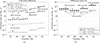Figure 15 Calculation time per frequency for the four types of transfer functions in Table 1. (a) First-order diffraction calculations (b) Calculation of diffraction orders 2–6.

$$\begin{array}{c}\hfill T_{\mathrm{calc}.,\mathrm{D}1}\propto n_{\mathrm{sources}}·n_{\mathrm{receivers}}·n_{\mathrm{edges}}.\end{array}$$(34)

In addition, the first-order diffraction calculations in this study are for a 2D geometry, which either is implemented with an explicit line source expression, equation (19), or as 501 monopoles in a 3D geometry of finite length, L. Thus, the calculation time dependence on frequency will behave differently for those two types of source types. For both types of sources, the calculation time will increase with frequency, but for the monopole expression also the edge length will affect the calculation time. The line source expression involves Bessel functions which are somewhat more expensive to compute for higher argument values⁷. On the other hand, when the line piston is modelled as a number of monopoles, then the edge will be a 3D edge of length L, so the factor kL affects the oscillation of the integrand and thus the computation time. In light of this, the following can be observed for results in Figure 15a:

• The calculation times generally increase with frequency, as expected. Ignoring the three jumps at 160 Hz, 500 Hz, and 1.25 kHz, the growth with frequency is clearly less for the TFs using line source expressions than for the TFs using monopoles. This difference reflects that the Bessel function computation is more benign than the oscillating integral computation for the monopole expressions.

• The huge difference in calculation times between the four types of transfer functions largely reflects the number of sources and receivers. The lowest curve segments has one line source and 2, 2, 5 or 11 receivers, respectively. The second lowest curve has one line source and 181 receivers etc.

• At the jumps, for three of the curves, the edges become shorter, see Table 2, which leads to a reduction in calculation time. At the same time, the number of secondary sources increases, for two of the three jumps, which gives a net increase in calculation time. For the curve denoted G(x_SS ← x_SS), the number of sources and the number of receivers increase at the two later jumps, so, for cases which require large number of secondary sources, the computation of the G(x_SS ← x_SS) TFs could typically dominate the calculations.

• The number of edges is very small for the chosen geometry, and the number of edges that are visible from the source and the receiver will not vary much across receiver positions. It can be noted that for a polyhedron, a receiver at the surface of the polyhedron (where the secondary sources are positioned) can only see the edges belonging to the polyhedral face which the receiver is placed at.

• As a rough estimate, based on the cost for computing the G(x_SS ← x_SS) TF, for a single monopole to a single receiver, at 50 Hz for a 40 m long edge, such that kL ≈ 37, using the chosen Matlab implementation, on the chosen computer hardware, the calculation is on the order of 2 ms. This calculation involves two edges of length 40 m.

6.2.2 Higher-order diffraction calculations

The calculation of higher-order diffraction uses a different algorithm than the first-order diffraction, and evaluates an integral equation with Gaussian quadrature. As seen in Table 2, two slightly different numbers of quadrature points, 399 and 449, along each edge were used. For Gaussian quadrature, the calculation time will not depend on frequency, only on the quadrature order, n_g, (which might, however, need to be higher for higher frequencies). The calculation cost for higher-order diffraction will be somewhat more complex than for first-order diffraction as given by equation (34). Thus, the four distinct calculation steps add up to the total cost as

$$\begin{array}{cc}\hfill T_{\mathrm{HOD}}& =T_{\text{source-term}}+T_{\text{set up H-matrix}}+n_{\text{diffr. order}}\hfill \\ \hfill & ·T_{\text{iterate H-matrix}}+T_{\text{prop. to field-points}}\hfill \\ \hfill & =C_1{n}_{\mathrm{sources}}·n_{\mathrm{g}}^2+C_2{n}_{\mathrm{g}}^3+C_3{n}_{\text{diffr. order}}{n}_{\mathrm{g}}^3\hfill \\ \hfill & +C_4{n}_{\mathrm{g}}^2{n}_{\mathrm{receivers}}.\hfill \end{array}$$(35)

It should be noted that n_sources in equation (35) refers to the number of sources which are added into a single transfer function calculation, such as when 501 monopoles are used to represent a line source. On the other hand, for G-TFs, one independent TF calculation has to be made for each secondary source. The total calculation times, T_HOD in equation (35), for the higher-order diffraction, including up to 6th order, are shown in Figure 15b for the same four types of TFs as in Figure 15a. The plotted calculation times are exactly the same for the four/five frequencies of each curve segments. A single value was computed and used for all frequencies in the plot since there is no dependence on frequency. The following observations can then be made about the higher-order diffraction:

• Both the H- and G-types of transfer functions must use 501 monopoles to represent the primary line source (H-TFs) or the line pistons (G-TFs). Also, as seen in equation (35), the number of receivers affects the total computation time only indirectly, and this fourth term in equation (35) turns out to have a small influence altogether. These two factors make the differences between TF types much smaller in Figure 15b than in Figure 15a.

• The jump at 160 Hz involved a reduction in quadrature order from 449 to 399, which reduced the calculation times. The jump at 1.25 kHz was associated with an increase in quadrature order to 449, which increased the calculation times.

• The calculation times for the G-TFs increased for the two jumps at 500 Hz and 1.5 kHz. The reason was that the number of secondary sources increased from 2 to 5, and from 5 to 11, respectively. The calculation times will be directly proportional to the number of secondary sources, as shown in Section 3.3.

As an additional analysis of the calculation of higher-order diffraction, the four steps in equation (35) were computed for different diffraction orders and different quadrature orders. This was done for the H(x ← x_S) TF. Keeping the number of sources (501 monopoles), quadrature order (399), and number of receivers (181) constant, but varying the diffraction order from 2 to 6 gave the calculation time results in Figure 15a. As seen in equation (35), the calculation time for the step “Iterate H-matrix" increases linearly with diffraction order. The other three steps should be independent of diffraction order except for the setting up of the H-matrix, which is not needed for the diffraction order 2: only the q₀-term in equation (7) is required. The slight dependence of diffraction order for the term “Propagate q-values to field points" is specific for this implementation. The double arrows indicate which steps depend on the number of sources and receivers.

In Figure 15b, calculation time values are given as function of quadrature order (per edge), with the number of sources (501), the number of receivers (181), and diffraction order (6) kept constant. Please note the logarithmic scales, which makes it quite clear that two of the four terms basically follow an n_g²-trend and the other two an n_g³-trend, as expected from equation (35). As in Figure 15a, the double arrows indicate the terms which are affected by the number of sources and receivers.

These results confirm that the point-to-point, 3D transfer function basis of the ESIE method significantly affects the cost for simulating a 2D case with this method. Furthermore, keeping the quadrature order, and diffraction order, as low as possible is important for optimizing the performance of the method, as shown by the timing results in Figure 16. Finally, for higher numbers of secondary sources than demonstrated here, the computation of the G_front = [G(x_SS ← x_SS)] matrix might dominate the computational load. Thus, the possibility to ignore higher-order diffraction, or even first-order diffraction, as demonstrated in Figure 14, might significantly increase the feasibility of the ESIE+SS method, but this would have to be evaluated for more cases.

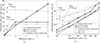Figure 16 Calculation time per frequency for the four steps of the calculation of higher-order diffraction, as given in equation (35). (a) THOD as function of diffraction order. The quadrature order was 399 for each edge. (b) THOD as function of quadrature order per edge. The diffraction order was 6.

7 Conclusions

A method, called ESIE+SS here, has been presented for the computation of scattering from a scattering object which is partly rigid and partly absorbing, using secondary sources and a diffraction-based method for the scattering of rigid bodies. The method is primarily valid for 3D geometries but expressions were presented for handling 2D problems with the ESIE and ESIE+SS methods.

The ESIE+SS method was evaluated for a 2D scattering object consisting of a rectangular box with a small impedance patch of a locally reacting material. FEM was used as a reference method and the ESIE+SS predicted sound pressures for the frequency range of 50 Hz to 2.5 kHz, along a semicircle around the object, and 90% of all the data points were within [ − 0.30,+0.32] dB of the reference FEM results. In a first evaluation step, the scattering of an all-rigid box was computed with the ESIE method, and 90% of the results were within [ − 0.20,+0.15] dB of the reference FEM results. For the ESIE and ESIE+SS computations, well-known numerical challenges occurred for some receiver positions, due to the slow convergence of the higher-order diffraction computations. The computational complexity was analyzed, confirming that the simulation of a 2D geometry with the ESIE+SS method is very inefficient. It was also found that the computation of transfer functions between all pairs of secondary sources might be the dominating cost. The possibility to ignore higher-order diffraction for those transfer functions mitigates that computational cost to some degree.

Acknowledgments

This research was funded by the Norwegian Defence Estates Agency.

Conflicts of interest

The authors declare no conflict of interest.

Data availability statement

Parts of the code used are available in GitHub, under the reference [28]. Other code, and results, are available on request from the corresponding author.

References

Appendix

The impedance values in the numerical example

In the numerical example, a porous absorber was modeled using Mechel’s model, as implemented in the NorFlag software [27]. The flow resistivity was 10 kPa s/m² and the porosity was set to 95%. The specific acoustic impedance values, normalized against ρ₀c, were as given in Table A.1.

All Tables

All Figures

	Figure 1 (a) The integral equation in equation (7) expresses that the edge source amplitude at edge point xe2, in the direction of edge point xe1, is given as an integral over contributions from all edge points xe which can see xe2. (b) An additional contribution, q0(xe1 ← xe2), is caused by the primary source S.
In the text

	Figure 2 The propagation of the edge source amplitude, q(xe1 ← xe2), to the receiver point R.
In the text

Figure 3 The secondary source approach in equation (10) adds (a) the sound field generated by the primary source S and the rigid scattering object, and (b) the sound fields radiated by secondary piston sources SSi with vibration velocities uSS,i, when pistons are set in a rigid scattering object. Only the geometrical acoustics components are illustrated; diffraction components should be added to both (a) and (b).

In the text

	Figure 4 First-order diffraction TF in 2D computed with the ref. expression, equation (19), and via a set of monopoles, equation (24), with and without source amplitude tapering. (a) The three TFs. (b) The error for the two monopole distributions.
In the text

	Figure 5 Geometrical parameters for the plane-wave + piston edge-wave model. (a) The plane wave component exists if the projection, xproj., onto the baffle of a receiver position, x, falls inside the piston, as is the case for position x1 but not for x2. (b) The edge wave uses a local spherical coordinate system, (r,θ,φ), for each position, xe, along the piston edges.
In the text

	Figure 6 Geometrical parameters for the edge-wave impulse response calculation for a line piston. The coordinates (ξ′,ψ′) are indicated for the calculation of the second edge’s contribution.
In the text

Figure 7 Geometrical details for the numerical example with a mostly rigid box, sized 3 m by 0.2 m, and a small patch with a locally reacting impedance boundary condition. A 2D point source is marked S. In (a), a semicircle of external receivers are placed at a radius of 3.1 m, with an angle step of 1 degree (not all are shown). In (b), two rows of receivers are placed at 1 cm and 2 cm distance (in the x-direction) from the box surface, in steps of 2 cm in the y-direction (not all are shown). An initial test case used an all-rigid box, without the impedance patch. The numerically most challenging receiver directions are marked with darker grey areas, and the more benign challenging directions are marked with lighter grey areas.

In the text

	Figure 8 The FEM used a 2D mesh of the area marked with grey in the figure.
In the text

Figure 9 Results for the scattering to the circle of receivers in Figure 7a for the all-rigid version of the box, for six example frequencies. Settings for the ESIE method were as in Table 2. The numerically most challenging receiver positions are marked with darker grey areas, and the more benign challenging positions are marked with lighter grey areas. (a) f = 50 Hz. (b) f = 125 Hz. (c) f = 250 Hz. (d) f = 500 Hz. (e) f = 1000 Hz. (f) f = 2000 Hz.

In the text

Figure 10 Median-quantile-values for the calculation error for (a) the all-rigid box, calculated with the ESIE method only, and (b) the box with an impedance patch, calculated with the ESIE+SS method. In both diagrams, the quantile values are given for 18 frequencies, including those not shown in Figures 9 and 11. The median and quantile values were based on the 181 receiver angle values shown in Figures 9 and 11. In (c) results for all frequencies and all 181 receiver positions were pooled into one dataset. Note the different scale in (c).

In the text

Figure 11 Results for the scattering to the circle of receivers in Figure 7b for the box with an impedance patch in Figure 7b, for six example frequencies. Settings for the ESIE+SS method were as in Table 2. The numerically most challenging receiver positions are marked with solid-line arrows, and the more benign challenging positions are marked with dotted-line arrows. (a) f = 50 Hz. (b) f = 125 Hz. (c) f = 250 Hz. (d) f = 500 Hz. (e) f = 1000 Hz. (f) f = 2000 Hz.

In the text

Figure 12 Results for the nearfield receivers in Figure 7b for the box with an impedance patch in Figure 7a, for three example frequencies: 50 Hz, 125 Hz and 250 Hz. Subfigures (a), (d), (g) show the sound pressure level, for an arbitrary source amplitude; (b), (e), (h) show the particle velocity, expressed in dB, whereas (c), (f), (i) show the specific acoustic impedance values. Settings for the ESIE+SS method were as in Table 2. Note the different scales between plots. (a) Lp,f = 50 Hz. (b) Lv,f = 50 Hz. (c) Zs,f = 50 Hz. (d) Lp,f = 125 Hz. (e) Lv,f = 125 Hz. (f) Zs,f = 125 Hz. (g) Lp,f = 250 Hz. (h) Lv,f = 250 Hz. (i) Zs,f = 250 Hz.

In the text

Figure 13 Results for the nearfield receivers in Figure 7b for the box with an impedance patch in Figure 7a, for three example frequencies: 500 Hz, 1 kHz and 1.6 kHz. Subfigures (a), (d), (g) show the sound pressure level, for an arbitrary source amplitude; (b), (e), (h) show the particle velocity, expressed in dB, whereas (c), (f), (i) show the specific acoustic impedance values. Settings for the ESIE+SS method were as in Table 2. Note the different scales between plots. (a) Lp,f = 500 Hz. (b) Lv,f = 500 Hz. (c) Zs,f = 500 Hz. (d) Lp,f = 1 kHz. (e) Lv,f = 1 kHz. (f) Zs,f = 1 kHz. (g) Lp,f = 2 kHz. (h) Lv,f = 2 kHz. (i) Zs,f = 2 kHz.

In the text

Figure 14 For the numerical example in Figures 7–13, in the frequency range which used two secondary sources: (a) The transfer function magnitudes Gfront and Grear for the SS 1← SS 1 combination. (b) The relative error for the G = Gfront + Grear transfer functions, when either only GA, or GA+first-order diffraction is included. (c) The relative error for the vSS secondary source amplitudes (due to symmetry both secondary sources get the same amplitude).

In the text

	Figure 15 Calculation time per frequency for the four types of transfer functions in Table 1. (a) First-order diffraction calculations (b) Calculation of diffraction orders 2–6.
In the text

	Figure 16 Calculation time per frequency for the four steps of the calculation of higher-order diffraction, as given in equation (35). (a) THOD as function of diffraction order. The quadrature order was 399 for each edge. (b) THOD as function of quadrature order per edge. The diffraction order was 6.
In the text

References

- J.J. Bowman, T.B.A. Senior, P.L.E: Uslenghi, eds.: Electromagnetic and Acoustic Scattering by Simple Shapes. North-Holland, Amsterdam, Netherlands, 1969. [Google Scholar]
- R.D. Ciskowski, C.A. Brebbia, eds.: Boundary element methods in acoustics. Computational Mechanics Publications, Southampton, UK, 1991. [Google Scholar]
- N.A. Gumerov, R. Duraiswami: A broadband fast multipole accelerated boundary element method for the three dimensional helmholtz equation. Journal of the Acoustical Society of America 125 (2009) 191–205. [Google Scholar]
- M. Zampolli, F.B. Jensen, A. Tesei: Benchmark problems for acoustic scattering from elastic objects in the free field and near the seafloor. Journal of the Acoustical Society of America 125 (2009) 89–98. [Google Scholar]
- L. Liu, D.G. Albert: Acoustic pulse propagation near a right-angled wall. Journal of the Acoustical Society of America 119 (2006) 2073–2083. [Google Scholar]
- A. Asheim, U.P. Svensson: An integral equation formulation for the diffraction from convex plates and polyhedra. Journal of the Acoustical Society of America 133 (2013) 3681–3691. [Google Scholar]
- S.R. Martin, U.P. Svensson, J. Slechta, J.O. Smith: Modeling sound scattering using a combination of the edge source integral equation and the boundary element method. Journal of the Acoustical Society of America 144 (2018) 131–141. [Google Scholar]
- H. Møller: Fundamentals of binaural technology. Applied Acoustics 36 (1992) 171–218. [CrossRef] [Google Scholar]
- G. Pavic, L. Du: Modelling of multi-connected acoustical spaces by the surface impedance approach, in: Internoise. Hamburg, 21–26 August, 2016, pp. 4278–4287. [Google Scholar]
- C. Zwikker, C.W. Kosten: Sound Absorbing Materials. Elsevier Publishing Company, Inc., New York, USA, 1949, pp. 132–135. [Google Scholar]
- H. Kuttruff: Room Acoustics, 4th edn. Spon Press, London, UK, 2000, pp. 159–163. [Google Scholar]
- P. Sjösten, U.P. Svensson, B. Kolbrek, K.B. Evensen: The effect of helmholtz resonators on the acoustic room response, in: BNAM. Stockholm, 20–22 June, 2016. [Google Scholar]
- G.P. Wilson, W.W. Soroka: Approximation to the diffraction of sound by a circular aperture in a rigid wall of finite thickness. Journal of the Acoustical Society of America 37 (1965) 286–297. [Google Scholar]
- U.P. Svensson, S. Sohrabi: Modeling sound transmission through apertures with diffraction, in: Internoise. Glasgow, 21–24 August, 2022. [Google Scholar]
- C.J. Bouwkamp: Diffraction theory. Reports on Progress in Physics 17 (1954) 35–100. [Google Scholar]
- W. Kropp, J. Bérillon: A theoretical model to investigate the acoustic performance of building facades in the low and middle frequency range. Acustica United with Acta Acustica 84 (1998) 681–688. [Google Scholar]
- E. Brandão, A. Lenzi, J. Cordioli: Estimation and minimization of errors caused by sample size effect in the measurement of the normal absorption coefficient of a locally reactive surface. Applied Acoustics 73 (2012) 543–556. [CrossRef] [Google Scholar]
- S.M. Kirkup, A. Thompson, B. Kolbrek, J. Yazdani: Simulation of the acoustic field of a horn loudspeaker by the boundary element-rayleigh integral method. Journal of Computational Acoustics 21 (2013) 1250020. [Google Scholar]
- U.P. Svensson, V. Henriksen, H. Olsen: Diffraction modeling for scattering objects with non-rigid surfaces, in: Forum Acusticum. Torino, 11–15 September, 2023. [Google Scholar]
- U.P. Svensson, P.T. Calamia, S. Nakanishi: Frequency-domain edge diffraction for finite and infinite edges. Acta Acustica United with Acustica 95 (2009) 568–572. [Google Scholar]
- A. Asheim, U.P. Svensson: Efficient evaluation of edge diffraction integrals using the numerical method of steepest descent. Journal of the Acoustical Society of America 128 (2010) 1590–1597. [CrossRef] [PubMed] [Google Scholar]
- I. Tolstoy: Exact, explicit solutions for diffraction by hard sound barriers and seamounts. Journal of the Acoustical Society of America 85 (1989) 661–669. [Google Scholar]
- M. Abramowitz, I.A. Stegun, eds.: Handbook of Mathematical Functions. Dover Publications, New York, USA, 1972, p. 364. [Google Scholar]
- G.R. Harris: Review of transient field theory for a baffled planar piston. Journal of the Acoustical Society of America 70 (1981) 10–20. [Google Scholar]
- U.P. Svensson, K. Sakagami, M. Morimoto: Line integral model of transient radiation from planar pistons in baffles. Acta Acustica United with Acustica 87 (2001)307–315. [Google Scholar]
- T.I. Laakso, V. Välimäki, M. Karjalainen, U.K. Laine: Splitting the unit delay. IEEE Signal Processing Magazine 13 (1996) 30–60. [CrossRef] [Google Scholar]
- T.E. Vigran: Software “Norflag”, previously sold by Norsonic AS. Not available anymore. [Google Scholar]
- U.P. Svensson: Complementary files to the publication “Handling impedance surfaces in diffraction modeling”. Available at: https://github.com/upsvensson/Edge-diffraction-Matlab-toolbox. [Google Scholar]