| Issue |
Acta Acust.
Volume 9, 2025
|
|
|---|---|---|
| Article Number | 37 | |
| Number of page(s) | 12 | |
| Section | Noise Control | |
| DOI | https://doi.org/10.1051/aacus/2025021 | |
| Published online | 23 June 2025 | |
Technical & Applied Article
Free field Active Noise Control system development using a 3D Finite Element based approach
Fraunhofer Institute for Structural Durability and System Reliability LBF Darmstadt Germany
* Corresponding author: This email address is being protected from spambots. You need JavaScript enabled to view it.
Received:
27
February
2024
Accepted:
16
May
2025
Abstract
This technical article presents a systematic methodology for efficient design, modeling, and validation of an Active Noise Control (ANC) system under free field conditions, aiming for global noise reduction. The presented three-dimensional (3D) Finite Element (FE) based simulation approach enables efficient ANC system design by generating valid data. It further allows for the optimization of control algorithms, evaluation of the attenuation performance, and methodical iteration of the overall concept design. A mock-up of a mobile ventilation system equipped with an ANC array serves as a demonstrator to present the stages of this methodology and its practicality. Starting with general concept considerations, the numerical modeling procedure, the different stages of verification and validation and concluding with an optimization task to achieve global noise reduction. The physical model of the demonstrator has been experimentally validated, and the efficiency of the developed ANC system confirmed through standardized sound power measurements in a semi-anechoic chamber. The findings reinforce the elaborated simulation process and demonstrate the real-world applicability of ANC systems. They also prove the potential for using simulations to develop free field 3D ANC systems capable of achieving global noise reduction.
Key words: Acoustic modeling / Free field radiation / Active Noise Control / Ventilation system / Digital development
© The Author(s), Published by EDP Sciences, 2025
 This is an Open Access article distributed under the terms of the Creative Commons Attribution License (https://creativecommons.org/licenses/by/4.0), which permits unrestricted use, distribution, and reproduction in any medium, provided the original work is properly cited.
1 Introduction
Noise control and low-noise design are becoming increasingly important in a wide range of applications. Noise has been ranked as the second most influential factor affecting human and environmental health [1]. Consequently, noise regulations have become more stringent, already leading to a reduction in noise exposure. However, over time this can lead to increased noise sensitivity, underlining the need for greater emphasis on comfort and a more silent living environment. To achieve these goals, development objectives, and to comply with increasingly stringent regulations, efficient and reliable simulation methodologies in digital environments are essential.
Acoustic measures and sound control methods can be categorized as either passive or active. Passive methods typically involve concepts of porous materials (e.g., fibers or foams [2]) which absorb and attenuate. They are most effective when they encapsulate or isolate the source [3]. In contrast, Active Noise Control (ANC) relies on an electroacoustic approach that incorporates additional sound sources, such as loudspeakers used together with digital signal processing [4–7]. Passive techniques typically excel in the higher frequency range (>1000 Hz) while active options are capable of managing a sound field in a broader low-frequency domain (<1000 Hz).
The potential of ANC results from extensive research on digital signal processing and algorithm optimization techniques. ANC is an expanding discipline including active and adaptive sound control and noise reduction. The field continues to grow, as evidenced by the increasing number of application scenarios and patents, despite its nearly 90-year history [8]. This growth has been exponential in the last decade [9]. The expansion of applications is driven by the increase in computing power and the decrease of hardware costs. Additionally, current research is bridging the gap to new areas such as artificial intelligence, virtual reality and digital twins. ANC is widely used, including headphones, transportation, medical industry, and human spaces [10]. Additionally, there is ongoing research on the manipulation of large soundscapes in the architectural environment [11]. Current research also focuses on practical applications such as open apertures, including windows or facade elements [12–14]. However, in practice, ANC still remains a specialized option for noise reduction due to physical and economic limitations and the effectiveness of control algorithms [10].
To enhance the effectiveness and to reduce development costs of an ANC system, it is advantageous to move the stages of design, testing, parametrization, and optimization into a digital environment. A 3D representation of a problem can be modeled using the (acoustic) Finite Element Method (FEM) and evaluated in conjunction with system and control simulations. An important factor in a simulation-based development process is to ensure accurate predictions of performance in real-world, free-field environments, and efficient optimization. This requires a deep understanding of the complex origins and interactions of acoustic radiation between the primary source, control sources, and surrounding elements. In the field of multiphysics research, Finite Element Analysis (FEA) serves as a powerful engineering tool for exploring coupled acoustic problems, providing an environment for analysis, optimization, and visualization. Using Finite Element (FE) modeling, sound propagation characteristics can be modeled in a way that accurately predicts the spatial and temporal variations of the sound field in both the near-field and far-field. By accurately considering boundary conditions, the simulation allows a realistic representation of the acoustic system, enabling digital ANC development.
1.1 Proposed methodology
The effectiveness of ANC systems in reducing noise from machine-like and similar components depends on several factors. One key aspect is the knowledge of the radiation behavior, which typically requires extensive measurement effort. For structural components, the use of accelerometers can reveal primary vibration patterns and determine the sources and pathways of structure-borne noise transmission. An effective acoustic technique for the identification of sound sources is the determination of the sound intensity on a grid. This method visualizes the distribution of sound energy and can highlight significant noise sources and unravel airborne sound paths. Despite their usefulness, these techniques are time-consuming and do not provide data that is directly applicable to ANC system design, as the measurement points typically differ from ANC sensor placement. This experimental approach provides only local insights into the radiation characteristics and requires more time to evaluate. Furthermore, a balance must be found between measurement resolution and experimental effort. For global source characterization, sound power can be used. However, if only this type of measurement is considered in the experimental characterization process, no valid conclusions about the local source composition can be drawn. However, sound power measurements can be used to globally validate a FE simulation model.
Sound power P is derived by taking Sound Intensity (SI) over a corresponding area, as indicated by the integral of the vectorial sound intensity I over the surface vector S. Following
 (1)
(1)
where the sound intensity I is the product of the sound pressure p and the particle velocity v integrated over the area of interest. While SI measurements are cumbersome to perform, FEA streamlines this process by accurately computing the velocity vectors, allowing sound power evaluation over arbitrary shapes of enveloping surfaces. This makes it easy to evaluate the contribution of a surface or panel to the global sound power.
To minimize measurement effort and machine downtime, the acoustic characterization process can be digitized. For this, standardized sound power measurement (e.g., following [15]) can be used to validate the corresponding simulation model. If the simulated sound power matches the experimental data it implies an accurate incorporation of the radiation characteristics in the simulation model, even when these characteristics are smeared globally. This allows a decomposition of the simulation model to identify specific radiating components. Moreover, an efficient evaluation of structural changes or the influence of additional parts ca be valued. Furthermore, a globally valid 3D acoustic FE model can provide data that can be used raw for ANC system design and enable conceptual studies. An illustration of a conventional characterization process and a digitized methodology is shown in Figure 1. While the standard approach needs the finished physical machine to identify issues and develop countermeasures, the FE-based approach allows preliminary simulation-based studies without physical prototypes. A simulation model validated afterwards can additionally provide reliable data for extensive concept studies, deferring the need for a physical machine until the implementation.
 |
Figure 1. Illustration of the development process over time using a conventional approach or a digitized characterization stage. In comparison to the conventional approach (1st row), the digitized stage can reduce characterization times, allowing for more optimization iterations in the same time (2nd row) – or can even reduce the development time considering the same optimization effort (3rd row). |
1.2 State of the art
In [16] an ANC system was installed in a ventilation window/duct, which resulted in significant extra attenuation. The simulations were based on an analytic model that was initially verified by FEA. The ANC system was analytically evaluated and further experimental results were discussed. However, no definitive comparison with the original predicted results was provided. An integrated ANC solution is proposed for a line-shaped heat ventilation unit in [17]. The retrofit design includes an additional duct that covers the original outlet. The authors used a numerical 3D FE-based design approach. However, they neither compare the results with an experimental setup nor propose specific modeling aspects.
A computational ANC study is proposed in [18, 19]. They investigated the physical limits of ANC with respect to an open aperture. The authors performed 2D FEM simulations using the Perfectly Matched Layer (PML) method to establish free field conditions. The study aimed to investigate the reduction of sound power in the far field based on the number of secondary sources. In [20, 21] the result were further discussed and elaborated. Elliott et al. [20] conducted a numerical investigation of the wave number approach for controlling a plane wave under normal and oblique incidence, resulting in a description of the geometry of secondary source distribution to achieve the best possible far-field attenuation.
A numerical model of an active headrest was introduced in [22, 23] discussed a virtual sensing ANC for aircraft seats using a functional link neural network. They conducted FE simulations and experimental tests. However, the numerical model remains unvalidated and uncalibrated.
In [24] a hybrid noise barrier with ANC was examined, using intensity probes and a sound intensity cost function to improve the far-field attenuation. Physical measurements were performed in addition to prior numerical simulations. Although no calibration was presented, the overall results were compared and accepted. However, some discrepancies between simulated and measured results were found. The authors of [25] presented an ANC barrier for outdoor noise, using iterative experiments and FE simulations to compare numerical and experimental results. Two experimental studies were assessed and the results were compared by presenting a numerical contour plot along with experimental data at discrete points at single frequencies. The authors presented compatible values and a numerical result for an outlook configuration using a well-described FE model. However, no calibration of the numerical model was presented.
This brief review of the use of FEA and design approaches shows that the authors unanimously appreciate the benefits of numerical investigations. However, none of them focus on a practical design scheme or numerical modeling specifically. Mostly, FEA is only used to obtain a general idea of the final solution rather than to create an accurate representation of the domain. In summary, basic FE models are used to perform numerical studies, while more advanced simulations can generate data for the control algorithms or provide reliable insights into what is likely to happen in the physical space. The authors of the present article are not aware of any contribution covering the entire process of establishing a validated 3D FE model, extracting transfer path data, numerically optimizing the ANC system, and then validating the attenuation performance.
2 Use case
This paper focuses on the design stages to develop an ANC system and details the entire process using a ventilation system as an example. Building on [26], which introduced a simulation-first approach for early acoustic design evaluation, this paper uses the same validated model. In [27] the Frequency Response Assurance Criterion (FRAC) was used for reference sensor location optimization based on Frequency Response Function (FRF) correlation to the error sensors. In [28] an optimized sensor placement strategy to achieve global noise reduction was presented. To locate error sensors for different frequency bands, heat maps were evaluated to show the correlation between error sensor locations and global radiated sound power. The present paper concludes this research with a summary of the steps and an experimental validation of the ANC systems.
The FE-based approach is presented in the context of a mobile ventilation system, as shown in Figure 2. In these systems, air is drawn in at the bottom and purified air is exposed at the top. Such machines are associated with high noise levels and can be annoying to people [30]. Noise is transmitted in two primary paths: structural vibrations and airborne sound. Structural vibrations are generated by the fan and transmitted through the machine housing. However, the dominant noise pathway is the airborne sound path, caused by the desired air exchange rate, which correlates with high velocity air turbulences at the fan. Concluding, the global noise level is predominantly influenced by the emission at the top outlet. This finding is crucial for the the development of an ANC system. An appropriate ANC system can intervene directly in the airborne sound path without significantly affecting the required airflow of the machine through passive measures.
Figure 3 shows the spectrum of measured sound pressure level of a mobile ventilation system. The amplitude response shows that the frequency bands with the highest levels are below 1000 Hz. Specifically, the 630 Hz band indicates the following level decrease. The most dominant bands are 100 Hz, 160 Hz and 315 Hz. Low frequencies below 80 Hz are excluded because this would require larger speakers. Therefore, the frequency bands that should be addressed for noise reduction are the third octave bands from 100 Hz to 630 Hz.
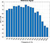 |
Figure 3. Measured sound pressure level from a reference mobile air purifier in third octaves. |
2.1 Active Noise Control system
For demonstration, a mock-up of a mobile ventilation system is used, as shown in Figure 4. On the left hand side it contrasts typical ventilation systems, such as industrial fans or mobile air purifiers, with the initial setup of the demonstrator. On the right hand side, this demonstrator replicates a mobile system with a wooden box design. A 3×3 array of secondary sound sources is placed in the outlet. The primary sound is generated by a loudspeaker at the bottom (shown in Fig. 4, right picture), emitting the original measured spectrum, Figure 3. The sound emitted at low frequencies forms a nearly spherical pattern that can be countered by a single loudspeaker. However, the actual machine noise is a mixture of fan and airflow sounds distributed throughout the system. At higher frequencies, the sound becomes more directional, forming lobes that require multiple loudspeakers to create the necessary beamforming [31]. By placing the loudspeakers at the outlet, where the airborne sound passes through, the secondary sound waves can be superimposed to recreate the primary sound field, essentially synthesizing the sound field.
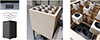 |
Figure 4. Illustration of typical industrial air outlets and mobile ventilation systems. Wooden box shows an initial state of an already established ANC setup, approximating an air purifier. |
From the general setup all further parameters for the operation of the ANC system follow. The distance between the loudspeakers and the microphones is critical for effectiveness of the ANC system, as explained in [20]. Secondary sources are placed closer than half the wavelength λ (Eq. (2)) of the highest frequency to tackle sound coming from an angle, while the distance could be larger for normally incident sound.
 (2)
(2)
Considering the frequency range of interest and the dimensions of the demonstrator, a spacing of l=200 mm was chosen, corresponding to a maximum frequency of 860 Hz. The error microphones capture the noise and serve as focal points for adjustment and calibration. They should placed far enough from the loudspeakers to avoid detecting evanescent modes – complex sound waves that fade with distance. The first spatial harmonic is attenuated by 20 dB after a certain distance z, depending on the spacing l. After Elliott et al. [20] this is given by
 (3)
(3)
with the wavenumber  . The largest value of z is required by the largest wavenumber, i.e., the smallest wavelength λmin corresponding to the highest frequency under consideration fmax. The simplification is based on a spacing of equation (2), which leads to
  . For the setup, this distance is at least z=85 mm. To account for uncertainties and to ensure that only propagating wave modes are detected, the closest error microphone plane is considered at a height of 100 mm above the secondary loudspeakers.
The reference microphones inside the box capture the noise and enable the ANC system to compute the anti-noise. Their placement is determined by maximizing the FRAC in relation to the error sensors. This ensures a high correlation with the optimization points and that the controller has enough time to respond.
2.1.1 Control algorithm
The ANC system is based on a broadband implementation of the normalized Least Mean Squares (LMS) algorithm with filtered reference signals (FxNLMS). Following the principles outlined in [4], the normalized LMS algorithm is designed to converge to the Wiener solution  , with the auto spectral density Sxx and cross spectral density Sxe under relatively lenient convergence criteria. Adaptation filters can be used to limit the adaptation to the specified frequency range, and their application to both the error e and reference x does not violate the convergence condition. This is evident in the frequency domain with the transfer function H. Equations (4) and (5) show that applying the same filter h to both signals leads to the same result W, equation (6).
 (4)
(4)
 (5)
(5)
 (6)
(6)
The real-time ANC system is modeled in Simulink, as shown in Figure 5. The system is segmented into five functional blocks, which include the digitization of the reference and error microphone signals by the Analogto-Digital Converter (ADC) and the output of the control signal by the Digital-to-Analog Converter (DAC). A dSpace ds2003 ADC unit and a ds2103 DAC unit, each with 32 channels, are used in the setup. The input is acquired with 12-bit resolution within a ±10 V range and the output generated with 14-bit resolution. Although the ADC is capable of 16-bit resolution, 12-bit is chosen to optimize conversion time, a critical factor for feed-forward control. Oversampling combined with digital anti-aliasing filters alleviates the need for sharp analog anti-aliasing filters, further reducing conversion time. Therefore, both the ADC and DAC stages operate at 12 kHz, doubling the control system's 6 kHz.
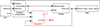 |
Figure 5. Simulink model of the active noise control scheme, simplified. |
The control system incorporates a feedback compensation mechanism to cancel any control signal picked up by the reference microphones. The adaptation block continuously refines the control filter parameters using the compensated reference signal x and the error signal e. As part of the adaptation block, the reference signal is passed through a plant model to obtain the filtered reference fx. The error signal represents the external noise emitted by the ventilation system. The amplitude of the control signal is carefully monitored to ensure that it remains within prescribed limits, and the control filter parameters are adjusted accordingly. The control block applies the adjusted filter parameters to the compensated reference signals to synthesize the control signal.
2.2 Numerical modeling
In [26], a detailed FE modeling approach for the demonstrator was proposed and validated with experimental results. There, a comprehensive overview of the FE model is given, describing, e.g., the mesh specifications and the simulation parameters. The FE model used is shown in Figure 6. It is based on the CAD geometry of the simplified ventilation system including the loudspeaker array described in Section 2.1. The FE model is a pure acoustic model. Thus, no two-way fluid-structure interactions are considered, only a one-way kinematic coupling is introduced by velocity excitation.
 |
Figure 6. Acoustic simulation model: excitation (1), interior (2), radiation space (3), reference microphones (4), secondary sources (5), error microphones (6). |
The model comprises three distinct regions: the excitation volume (1), the air inside the box (2), and a free field radiation region (3) to avoid reflections. The reference sensors of the ANC system are positioned in the region indicated by (4), the secondary source array is indicated by (5), and the error sensors (6) are located above the secondary source array. The reason for employing an all-acoustic model is based on the negligible impact of the acoustic medium on the wooden box and the absence of significant structural vibrations in this context. It is assumed that the radiation emanating from the wooden box can be disregarded. Nevertheless, two-way coupling would result in damping effects due to partial absorption. To account for these effects, a frequency-independent absorption coefficient α of 5% is assumed based on a literature review [32]. This frequency-independent absorption is a surface impedance boundary condition that leads to acoustic damping. This is a simplification for non-normally incident sound waves, but provides sufficient results in this case.Additionally, in the later introduced 2nd concept, acoustic foam is considered inside the demonstrator. A porous material model according to Delany-Bazley [33] was used to account for the effects. This empirical one-parameter model requires only the fluid resistivity σres in addition to the air constants. The fluid resistivity is estimated from the frequency dependent absorption coefficient α(f) of the material as given in the manufacturer's data sheet.
Given that the model is symmetric with an open space on one side, it follows that no anti-symmetric eigenmodes can occur. Consequently, only a quarter of the model is necessary. In [27], region (4) was considered in order to identify suitable reference sensor locations, depending on the error sensor signal. As the signal emitted by the secondary sources can only be as accurate as the signal sensed at the reference sensors, the greater the correlation between the reference and error signals, the greater the ANC effect. The FRAC was employed for this purpose. In [28], region (6) was evaluated in order to couple the error sensor signals with a global value to derive valuable error sensor locations.
The loudspeaker excitation in the FEA is introduced by a velocity boundary condition on the diaphragm, see Figure 7. However, this one-way kinematic excitation results in frequency independent radiation characteristics, while physical loudspeakers show frequency dependent behavior due to their electrodynamic properties. To accurately simulate these characteristics, it is necessary to determine the transfer function of a loudspeaker in its enclosure (Fig. 8) and include them in the simulation. This can be done analytically using a lumped parameter model, as shown in Figure 7, with the methodology proposed in [34, 35]. The use provides a numerically efficient and valid prediction of the simulation, allowing accurate data extraction for ANC design.
 |
Figure 7. Loudspeaker enclosing geometry and lumped-parameter model for an analytic description of a transfer function of a loudspeaker in a housing, after [35]. |
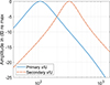 |
Figure 8. Amplitude transfer function of the primary and secondary sources using a lumped-parameter-model. |
In order to design an effective ANC controller, it is necessary to conduct system identification experiments. These experiments typically involve applying a broadband signal and measuring the response at the microphones. In FEA, frequency domain or transient simulations can be performed, for example with harmonic, noise, or impulse excitation. Time-domain simulations were conducted using FE software to model the transient processes directly and utilize the obtained impulse response from the FE model as Finite Impulse Responses (FIR) filter in the ANC controller design process. In [26], the authors provided detailed information on how to efficiently and validly determine the necessary time-domain simulation parameters a priori, e.g., time step size Δt and total simulation time Tsim. A verification and validation approach is detailed as well.
2.2.1 Physical validation
To validate the simulation, a physical validation of the original initial setup is performed. The results of simulation and experiment are compared by transforming the transient simulation results into the frequency domain. Figure 9 shows this comparison for a local transfer function from the primary excitation to an exemplary reference microphone. The results show good agreement, both in terms of characteristics and sound pressure level. An investigation of corresponding modes can be found in [27]. The unwrapped phase response (in radians) shows the simulation slightly above the experiment, indicating a lower group delay. This is also visible in the group delay plot. In terms of active control, a lower group delay in the simulation indicates that less time is available for control computation than is actually available. However, in summary, the differences are marginal and the lower group delay correlates with a stronger damping of the real system.
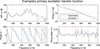 |
Figure 9. Comparison of an exemplary transfer function by magnitude and phase response between experiment and simulation for the primary excitation to an error sensor. On the left: magnitude in dB (top) and phase in degree (bottom). On the right: unwrapped phase in radians (top) and group delay (bottom). |
To validate the global acoustic behavior, the sound power level is evaluated with the proposed ventilation noise. The sound power is measured according to DIN EN ISO 3744 [15] in a semi-anechoic chamber. However, some measurement restrictions due to the environment have to be taken into account. Thus, the measurement follows the instructions of [15], but is not fully compliant in some frequency bands. A rectangular enveloping surface with a total of 13 microphones was used. The upper surface was divided into four areas, thus introducing four additional microphones. Figure 10 shows the measurement setup.
 |
Figure 10. Demonstrator in a semi-anechoic chamber for sound power evaluation. The left and middle images show the ANC array, the error sensors above, and a view inside the box with passive treatments. The right image shows the demonstrator in the center of the cuboid enveloping surface for sound power measurements. |
The comparison of the sound power level between experiment and simulation is shown in Figure 11. A very good correlation can be seen in the targeted frequency bands. The general trend is correctly estimated. The largest deviations show an error of about 2 dB, but are mostly ≤1 dB. This indicates that the model is well established and that relevant noise mechanisms are included. Therefore, the model can be considered as valid and used to infer acoustic effects to determine a numerically optimized ANC design.
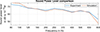 |
Figure 11. Comparison of sound power level predicted by the simulation and experimentally measured. |
2.3 Optimization procedure
The optimization procedure considers both fixed and variable constraints. First, the ANC array is fixed in its configuration, which is considered to be optimal according to Section 2.1. However, the sensor locations, their arrangement, and the ANC target of global, not only local, sound power reduction are included in the optimization procedure. In [27] simulative evaluations have been proposed for the placement of the reference sensors depending on the error sensor signals. The considerations include the correlation of the reference and error signals using the FRAC to compare and evaluate the correlation – without a specific optimizer. In [27] these considerations were extended to the correlation of the error signals to a global indicator – the sound power. To achieve global noise reduction, not only at local (error sensor) points, a simulation framework was proposed to relate the error sensor locations to a global value. By decomposing the sound power relative to the corresponding area of each node in a panel and deriving the normal vector component, the contribution to the sound power for each frequency can be quantified. This can further be normalized to the maximum value for that frequency. Since the sound power distribution varies slightly across frequencies, dominant distributions can be identified by computing the mean across frequency bands. Figure 12 shows the mean sound power contribution across these bands, evaluated at the error plane 100 mm above the secondary sources, as shown on the right in Figure 6. As stated in [28], the visualization of the simulated intensity distribution provides valuable insights into the acoustic behavior of the system.
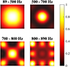 |
Figure 12. Normalized sound power contributions for possible error sensor positions. Averaged over frequencies with similar behavior. Top view with mirrored results of the quarter model. |
The evaluation shows that one microphone placed centrally above the opening can adequately cover a frequency range up to 500 Hz. This position is still dominant up to 700 Hz, where the corners of the box also become radiation areas. The corners become more dominant in the 700 to 800 Hz frequency range, and remain so for higher frequencies. Beyond 800 Hz, additional locations at the edge centers show an increased contribution, while the center location becomes nearly negligible. Considering frequencies included in the 800 Hz third octave, the locations shown in Figure 13 are determined to capture most of the radiated sound power characteristics with the minimum number of sensors required.
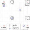 |
Figure 13. Top view of the quarter model with the final arrangement strategy for the optimized ANC concept. |
With the fully determined ANC concept, the control simulation can predict the possible noise reduction. Figure 14a shows the prediction of the initial concept and Figure 14b shows the prediction of the possible attenuation of the optimized concept over one-third octave bands at the error sensor locations, according to [28].
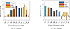 |
Figure 14. Simulated SPL reduction at error sensors by ANC for 1st (left) and 2nd (right) concept. (a) 1st concept. (b) 2nd concept. |
3 Evaluation
To validate the simulative predictions, sound power measurements in accordance with DIN EN ISO 3744 [15] are conducted for the two ANC configurations: the initial configuration as presented in [26] and the second one with the sensor arrangement optimized for global sound power as presented in [28] and further proposed in this article. Figures 15 and 16 illustrate the measured sound power levels. In contrast to Figures 14a and 14b, the global sound power is utilized instead of the local sound pressure at the error sensors. This is a result of efficiency considerations. It would have been necessary to perform several additional simulations to apply the control signal back in the FE simulations. However, at the beginning of the optimization process, the results from the error sensors provide sufficient insight into the sound distribution to continue with the sound power optimization afterwards. This allows for a comparison of the characteristics, which shows that the overall prediction of both states is in good agreement with the simulated trend. Furthermore, it is evident that the optimized concept has successfully shifted the ANC effect to lower frequency bands.
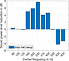 |
Figure 15. Sound power reduction of 1st concept. |
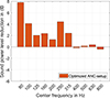 |
Figure 16. Sound power reduction of 2nd concept. |
However, it is evident that the local error sensor reduction levels cannot be achieved globally, as the measurement study has demonstrated. Only half of the expected reduction (in dB) has been verified globally in the experiment. This shortfall is likely due to the differences between the local and global sound field. In addition, other key factors were identified: the loudspeaker power appears to be insufficient to achieve the predicted performance. Furthermore, frequency bands above 400 Hz appear to have no effect or even show a negative reduction, suggesting potential issues with causality or non-linear effects.
Comparing the two concepts, both have their strengths in different frequency bands. The optimized concept offers its strength primarily in the low frequency range, confirming the suitability of ANC in these frequency bands. However, it would be advantageous to obtain the performance of both, the original and the optimized schemes simultaneously for a more homogeneous and frequency-independent sound power reduction.
4 Conclusions
This paper proposed a comprehensive simulation methodology to develop ANC concepts under free field conditions with the goal of global sound power attenuation. For this purpose, the authors previous research work was highlighted and the most important details were shared again in this contribution to encompass all components of the methodology. In addition to the FEM development and optimization approach, standardized sound power measurements were performed to validate the designed ANC concepts. It has been found that the 3D FE based development approach delivers a suitable framework for free field ANC system design tasks, leading to physical ANC systems with similar characteristics as simulated. The comparative analysis of the two ANC concepts revealed a fundamental congruence between the predicted characteristics and the final sound power measurements. This confirms the chosen accuracy of the simulations and the ability to predict the overall behavior of the ANC system across multiple frequency bands. This is a positive indicator of the simulation framework as an efficient approach in the development and optimization of ANC systems.
Despite these encouraging results, the study also identified discrepancies that require further investigation. The influence of complex room acoustics on the ANC performance has become apparent due to the non-ideal semi-anechoic room. In addition, the accuracy of the sound measurement equipment and the calibration process play a critical role in achieving accurate results, especially at higher frequencies where spatial resolution is critical. Electronic components, such as signal processors and amplifiers, may have limitations that were not fully anticipated in the simulations. These limitations can affect the ANC capabilities of the system. In addition to the mentioned technical limitations, another important aspect to consider in the research and development of ANC systems is the integration of advanced algorithms and machine learning techniques. By incorporating these cutting-edge technologies, ANC systems can adapt and learn from real-time data, improving their ability to cancel unwanted noise in different environments. In addition, it would be beneficial to mathematically define an advanced cost function that could be evaluated using available state-of-the-art optimizers.
The development of ANC systems should also focus on energy efficiency. By optimizing the power consumption of ANC components, it will be possible to reduce their environmental impact. This can be achieved through the use of low-power hardware components and intelligent power management techniques. Finally, to ensure widespread adoption of ANC systems, it is essential to address potential cost barriers. By streamlining the manufacturing process and leveraging economies of scale, ANC technology can become more accessible to a wider range of applications. In summary, further research and development efforts should focus not only on overcoming technical limitations, but also on integrating advanced algorithms, exploring diverse application areas, improving energy efficiency, and addressing cost considerations. This allows ANC systems to reach their full potential and revolutionize the way we experience and interact with sound.
Funding
The authors would like to thank the Fraunhofer Society for funding the research, and their colleagues at Fraunhofer LBF and IBP for their invaluable insights on various technical aspects.
Conflicts of interest
The authors declare that they have no conflict of interest.
Data availability statement
The data that support the findings of this study are available from the corresponding author on request.
References
- World Health Organization. Regional Office for Europe: Burden of Disease from Environmental Noise: Quantification of Healthy Life Years Lost in Europe. World Health Organization Regional Office for Europe, Copenhagen, 2011 [Google Scholar]
- J.F. Allard: Propagation of Sound in Porous Media: Modelling Sound Absorbing Materials, 2nd edition. Wiley, Chichester, 2009 [CrossRef] [Google Scholar]
- M. Abele, M. Budnik: Simulation and validation of the isolation-effect of acoustic encapsulation concepts based on a generic electric motor housing, in: SAE Technical Paper Series, SAE Technical Paper Series. SAE International400 Commonwealth Drive, Warrendale, PA, United States, 2023 [Google Scholar]
- S.M. Kuo, D.R. Morgan: Active Noise Control Systems: Algorithms and DSP Implementations. John Wileys & Sons, New York, 1996 [Google Scholar]
- P.A. Nelson, S.J. Elliott: Active Control of Sound, paperback edition, 4. print, [nachdr.] edition. Academic Press, San Diego, 2000 [Google Scholar]
- S.J. Elliott: Signal Processing for Active Control. Signal Processing and its Applications. Academic Press, San Diego, 2000. Transferred to digital printing 2005 edition [Google Scholar]
- C.H. Hansen: Active Control of Noise and Vibration, 2nd edition. CRC Press/Taylor & Francis Group, Boca Raton, 2012 [Google Scholar]
- P. Lueg: Process of silencing sound oscillations. U.S. Patent 2043416, June 09, 1936 [Google Scholar]
- D.Y. Shi, B. Lam, W.-S. Gan, J. Cheer, S.J. Elliott: Active noise control in the new century: the role and prospect of signal processing, in: Inter-Noise, 2023 [Google Scholar]
- Y. Kajikawa, W.-S. Gan, S.M. Kuo: Recent advances on active noise control: open issues and innovative applications. APSIPA Transactions on Signal and Information Processing 1, 1 (2012) e3 [CrossRef] [Google Scholar]
- B. Lam, W.-S. Gan, D.Y. Shi, M. Nishimura, S. Elliott: Ten questions concerning active noise control in the built environment. Building and Environment 200 (2021) 107928 [CrossRef] [Google Scholar]
- T. Pàmies, J. Romeu, M. Genescà, R. Arcos: Active control of aircraft fly-over sound transmission through an open window. Applied Acoustics 84 (2014) 116–121 [CrossRef] [Google Scholar]
- B. Lam, D.Y. Shi, W.-S. Gan, S.J. Elliott, M. Nishimura: Active control of broadband sound through the open aperture of a full-sized domestic window. Scientific Reports 10, 1 (2020) 10021 [CrossRef] [PubMed] [Google Scholar]
- B. Lam, D.Y. Shi, V. Belyi, S. Wen, W.-S. Gan, K. Li, I. Lee: Active control of low-frequency noise through a single top-hung window in a full-sized room. Applied Sciences 10, 19 (2020) 6817 [CrossRef] [Google Scholar]
- DIN EN ISO 3744:2011-02: Akustik – Bestimmung der Schallleistungs- und Schallenergiepegel von Geräuschquellen aus Schalldruckmessungen – Hüllflächenverfahren der Genauigkeitsklasse 2 für ein im Wesentlichen freies Schallfeld über einer reflektierenden Ebene; Deutsche Fassung EN_ISO_3744:2010. Berlin [Google Scholar]
- H. Huang, X. Qiu, J. Kang: Active noise attenuation in ventilation windows. The Journal of the Acoustical Society of America 130, 1 (2011) 176–188 [CrossRef] [PubMed] [Google Scholar]
- S. Lesoinne, J.-J. Embrechts, G. Vatin, B. Ganty, Y. Detandt: Numerical acoustic modelling of a ventilation unit by 3D FEM and application to the design of an ANC feedforward system, in: M. Ochmann, M. Vorländer, J. Fels, Eds. Proceedings of the 23rd International Congress on Acoustics. Deutsche Gesellschaft für Akustik, Berlin, Germany, 2019 [Google Scholar]
- B. Lam, S. Elliott, J. Cheer, W.S. Gan: The physical limits of active noise control of open windows, in 12th Western Pacific Acoustics Conference (06/12/15–10/12/15), 2015, 12 pp. [Google Scholar]
- S. Elliott, J. Cheer, B. Lam, C. Shi, W.-S. Gan: Controlling incident sound fields with source arrays in free space and through apertures, in: 24th International Congress on Sound and Vibration (23/07/17–27/07/17), 2017, 7 pp. [Google Scholar]
- S.J. Elliott, J. Cheer, L. Bhan, C. Shi, W.-S. Gan: A wavenumber approach to analysing the active control of plane waves with arrays of secondary sources. Journal of Sound and Vibration 419 (2018) 405–419 [CrossRef] [Google Scholar]
- B. Lam, S. Elliott, J. Cheer, W.-S. Gan: Physical limits on the performance of active noise control through open windows. Applied Acoustics 137 (2018) 9–17 [CrossRef] [Google Scholar]
- J. Bean, N. Schiller, C. Fuller: Numerical modeling of an active headrest, in: Proceedings of the INTER-NOISE and NOISE-CON Congress and Conference Proceedings. Vol. 255. Institute of Noise Control Engineering (2017) 4065–4075 [Google Scholar]
- D. Mylonas, A. Erspamer, C. Yiakopoulos, I. Antoniadis: A virtual sensing active noise control system based on a functional link neural network for an aircraft seat headrest. Journal of Vibration Engineering & Technologies 12, 3 (2024) 3857–3872 [CrossRef] [Google Scholar]
- N. Han, X. Qiu: A study of sound intensity control for active noise barriers. Applied Acoustics 68, 10 (2007) 1297–1306 [CrossRef] [Google Scholar]
- F. Borchi, M. Carfagni, L. Martelli, A. Turchi, F. Argenti: Design and experimental tests of active control barriers for low-frequency stationary noise reduction in urban outdoor environment. Applied Acoustics 114 (2016) 125–135 [CrossRef] [Google Scholar]
- M. Budnik, V. Mees: Efficient simulative design, verification, and experimental validation of an active noise control measure for airborne sound radiation, in: Aachen Acoustics Colloqium AAC. RWTH Aachen, 2022, pp. 159–168 [Google Scholar]
- M. Budnik, V. Mees: Simulationsbasierte ermittlung der anordnung von mikrofonen und lautsprechern bei aktivem schallschutz, in: Tagungsband, DAGA 2023 – 49. Jahrestagung für Akustik. Ed. by O. von Estorff and S. Lippert. Berlin: Deutsche Gesellschaft für Akustik e.V, 2023, pp. 434–437 [Google Scholar]
- M. Budnik, V. Mees: Simulation-based design strategy and experimental validation of an active noise control setup simulation-based design strategy and experimental validation of an active noise control setup, in: Proceedings of Forum Acusticum 2023. European Acoustics Association, Torino, 2023, pp. 3643–3650 [Google Scholar]
- Kurt Hüttinger GmbH & Co. KG: Luftklar luftreiniger hepa 1800, 2021 [Google Scholar]
- D. Beer, F. Paul, B. Fiedler, J. Rohlfing, K. Bay, J. Torge, J. Millitzer, C. Tamm, Eds.: Luftreinigungsgeräte – akustische Anforderungen und Optimierungsmöglichkeiten, 2022 [Google Scholar]
- M. Möser: Engineering Acoustics. Springer Berlin Heidelberg, Berlin, Heidelberg, 2009 [CrossRef] [Google Scholar]
- J. Smardzewski, T. Kamisiński, D. Dziurka, R. Mirski, A. Majewski, A. Flach, A. Pilch: Sound absorption of wood-based materials. Holzforschung 69, 4 (2015) 431–439 [CrossRef] [Google Scholar]
- M.E. Delany, E.N. Bazley: Acoustical properties of fibrous absorbent materials. Applied Acoustics 3, 2 (1970) 105–116 [Google Scholar]
- E. Terhardt: Akustische Kommunikation. Springer Berlin Heidelberg, Berlin, Heidelberg, 1998 [CrossRef] [Google Scholar]
- M. Rossi: Audio. Électricité. Presses polytechniques et universitaires romandes and [Diff. Géodif], Lausanne and [Paris], 2007 [Google Scholar]
Cite this article as: Budnik M. & Mees V. 2025. Free field Active Noise Control system development using a 3D Finite Element based approach. Acta Acustica, 9, 37. https://doi.org/10.1051/aacus/2025021.
All Figures
|
Figure 1. Illustration of the development process over time using a conventional approach or a digitized characterization stage. In comparison to the conventional approach (1st row), the digitized stage can reduce characterization times, allowing for more optimization iterations in the same time (2nd row) – or can even reduce the development time considering the same optimization effort (3rd row). |
| In the text | |
 |
Figure 2. Illustration of a mobile air purifier, based on [29]. Bottom: air inlet. Top: air outlet. |
| In the text | |
|
Figure 3. Measured sound pressure level from a reference mobile air purifier in third octaves. |
| In the text | |
|
Figure 4. Illustration of typical industrial air outlets and mobile ventilation systems. Wooden box shows an initial state of an already established ANC setup, approximating an air purifier. |
| In the text | |
|
Figure 5. Simulink model of the active noise control scheme, simplified. |
| In the text | |
|
Figure 6. Acoustic simulation model: excitation (1), interior (2), radiation space (3), reference microphones (4), secondary sources (5), error microphones (6). |
| In the text | |
|
Figure 7. Loudspeaker enclosing geometry and lumped-parameter model for an analytic description of a transfer function of a loudspeaker in a housing, after [35]. |
| In the text | |
|
Figure 8. Amplitude transfer function of the primary and secondary sources using a lumped-parameter-model. |
| In the text | |
|
Figure 9. Comparison of an exemplary transfer function by magnitude and phase response between experiment and simulation for the primary excitation to an error sensor. On the left: magnitude in dB (top) and phase in degree (bottom). On the right: unwrapped phase in radians (top) and group delay (bottom). |
| In the text | |
|
Figure 10. Demonstrator in a semi-anechoic chamber for sound power evaluation. The left and middle images show the ANC array, the error sensors above, and a view inside the box with passive treatments. The right image shows the demonstrator in the center of the cuboid enveloping surface for sound power measurements. |
| In the text | |
|
Figure 11. Comparison of sound power level predicted by the simulation and experimentally measured. |
| In the text | |
|
Figure 12. Normalized sound power contributions for possible error sensor positions. Averaged over frequencies with similar behavior. Top view with mirrored results of the quarter model. |
| In the text | |
|
Figure 13. Top view of the quarter model with the final arrangement strategy for the optimized ANC concept. |
| In the text | |
|
Figure 14. Simulated SPL reduction at error sensors by ANC for 1st (left) and 2nd (right) concept. (a) 1st concept. (b) 2nd concept. |
| In the text | |
|
Figure 15. Sound power reduction of 1st concept. |
| In the text | |
|
Figure 16. Sound power reduction of 2nd concept. |
| In the text | |
Current usage metrics show cumulative count of Article Views (full-text article views including HTML views, PDF and ePub downloads, according to the available data) and Abstracts Views on Vision4Press platform.
Data correspond to usage on the plateform after 2015. The current usage metrics is available 48-96 hours after online publication and is updated daily on week days.
Initial download of the metrics may take a while.