| Issue |
Acta Acust.
Volume 9, 2025
|
|
|---|---|---|
| Article Number | 36 | |
| Number of page(s) | 12 | |
| Section | Acoustic Materials and Metamaterials | |
| DOI | https://doi.org/10.1051/aacus/2025019 | |
| Published online | 11 June 2025 | |
Scientific Article
Transient study of an optimized waveguide sonic black hole with wave focusing properties
1
Institute of Mechanics and Mechatronics, TU Wien Getreidemarkt 9 1060 Vienna Austria
2
FLOW, Engineering Mechanics, KTH Royal Institute of Technology Osquars Backe 18 SE-100 44 Stockholm Sweden
3
Department of Computing Science, Umeå University MIT-huset SE-90 187 Umeå Sweden
4
Department of Mathematics and Computer Science, Karlstad University Universitetsgatan SE-651 88 Karlstad Sweden
5
Institute of Fundamentals and Theory in Electrical Engineering (IGTE), TU Graz Inffeldgasse 18 8010 Graz Austria
* e-mail: florian.toth@tuwien.ac.at
Received:
10
December
2024
Accepted:
9
May
2025
Sonic black holes (SBHs) are waveguides intended to slow down the wave propagation speed and focus the energy towards the end of the device. However, the extent to which these effects occur, as well as the degree of wave dispersion introduced, has not been systematically quantified. This article investigates these aspects through transient finite-element computations, analyzing the properties of a novel, numerically optimized SBH with enhanced wave-focusing capabilities. The investigation utilizes the lossless acoustic wave equation as well as a linearized compressible flow formulation to account for viscothermal losses. We analyze the wave focusing and filtering properties of the SBH by monitoring the pressure amplitude and the transmission and reflection coefficients. Moreover, we examine the effective wave propagation speed along the centerline of SBH and assess the similarity of pressure wave packets using cross-correlations. Our results reveal that the optimized SBH not only enhances wave focusing but also on average effectively slows down wave propagation, demonstrating the device's potential as a true sonic black hole. By investigating two crucial aspects – wave-slowing effect and signal dispersion – that were not previously explored, we provide a deeper understanding of the device's functionality and operational mechanisms, including how its design influences wave-focusing performance and local wave speed.
Key words: Sonic black hole / Wave focusing / Wave slowdown / FEM
© The Author(s), Published by EDP Sciences, 2025
 This is an Open Access article distributed under the terms of the Creative Commons Attribution License (https://creativecommons.org/licenses/by/4.0), which permits unrestricted use, distribution, and reproduction in any medium, provided the original work is properly cited.
1 Introduction
The acoustic black hole (ABH) effect is a novel concept that has been extensively studied over the last couple of decades to design passive devices aimed at attenuating and controlling the propagation of acoustic waves across various applications [1]. Initially proposed by Mironov [2], the ABH effect involves achieving a broadband, gradual slowing of the transverse wave propagation speed in a beam or plate through a gradual reduction of its thickness. Theoretically, as the thickness smoothly reduces to zero, the propagation speed tends to zero, effectively trapping the waves within a finite-length device, which inspired the term “black hole” for this effect. The slowing effect in a beam ABH leads to a wave focusing effect with large amplitudes of the transverse waves at the tip of the beam. This focusing effect can be utilized to achieve broadband absorption by attaching a small amount of damping material at the tip of the beam. Therefore, structural ABHs have been studied mostly for structural vibration suppression [3–6], since the device makes highly effective use of the damping material. However, the focusing effect of ABHs can also be used in a variety of other applications, such as energy harvesting [7–10], signal enhancement and weak signal sensing [11–13], and wave focusing and acoustic lensing [14, 15].
Mironov and Pislyakov [16] later argued that the same wave focusing and slowing effect can be achieved for sound wave propagation in a cylindrical waveguide with a gradually varying radius and a purely compliant wall admittance according to a power-law profile. They proposed a fixed-radius cylindrical waveguide containing a set of rings separated by cavities as a practical realization of such a device, which they later referred to as a sonic black hole (SBH) [18]. Here we will use the term ABH to refer to devices where waves propagate in elastic solids, and SBH for devices where waves propagate in (acoustic) fluids. As depicted in Figure 1, the design proposed by Mironov and Pislyakov [16], also known as the ribbed SBH, is intended to create a strong wave focusing effect towards the end. It was expected that a small amount of damping material at the end of the waveguide would efficiently absorb the incoming sound waves similarly to structural black holes. This expectation turned, unfortunately, out to be false in practice [19]. However, many studies have shown that the viscothermal (also called thermoviscous) losses in air are sufficient to achieve broadband absorption using the ribbed design of SBHs [20, 21].
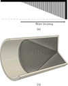 |
Figure 1. The ribbed design of a sonic black hole proposed by Mironov and Pislyakov [16] with an intention to create a wave focusing effect towards the end of the waveguide. Figure modified from Mousavi et al. [17]. (a) Axi-symmetrical model; (b) A 3D visualization |
Although SBHs have been introduced more than 20 years ago, novel variations and applications have been continuously introduced. Most works feature the classical ribbed design [22, 23], to which many variations have been presented: From micro perforated panels (MPPs) covering the SBH [22, 24–27], to perforations within the ribs [28, 29] to the addition of porous material [30] or a terminating Helmholtz resonator [31] many options for improving the absorption characteristics of the design have been suggested. The idea of a continuously changing impedance has been used in other design variations like an arrangement of folded cavities [32], rainbow-silencers [33, 34] or in periodic arrangements [35]. Furthermore, SBHs have been used in several applications, from sound mitigation in ducts [33, 34, 36] or windows [37] to acoustic energy harvesting [25].
Recently, it has been shown that the wall admittance model used by Mironov and Pislyakov [16] to design the ribbed SBH breaks down at higher frequencies, for which the wave focusing property is lost [38, 39]. Still, broadband absorption has been reported due to a completely different mechanism than intended, namely, radial resonances in the cavities appearing closer and closer to the waveguide entrance with increasing frequency. Note that the black-hole property of a monotonically decreasing wave propagation speed, which the ribbed SBH was supposed to possess, relied on the assumed gradually increasing pure compliant wall admittance. The presence of resonances shows that this assumption is false, and wave slowing can thus occur only for very low frequencies, below all resonances, where compliance dominates. Thus, the ribbed design is more of an acoustic absorber with distributed loss mechanisms than a black hole with wave focusing capabilities [39, 40]. Nevertheless, ribbed SBHs are being studied for broadband absorption in many different applications [41–46].
Because the ribbed design is incapable of creating wave focusing and, therefore, not an SBH, Mousavi et al. [17] attempted a first conceptual design of an SBH through computational design optimization. The aim was to create a true wave focusing device, analogous to the structural ABH, for sound waves in the air. For this aim, a density-based topology optimization approach was employed, capable of taking boundary viscothermal losses into account [17, 47]. Figure 2 illustrates the axisymmetric setup. A planar incoming wave is assumed at the waveguide entrance Γin. The objective of the design optimization is to concentrate the incoming wave energy at a small focusing area ΓT towards the end of the waveguide. The frequency-domain mathematical model involves the Helmholtz equation for the acoustic pressure in the air region together with a viscothermal boundary condition at the interface Γw to solid material.
 |
Figure 2. The conceptual setup for the design optimization problem. A plane wave enters Γin, and the problem is to place solid material Ωs in the region illustrated with a grid so that the acoustic power is maximized in the target region ΓT. Figure modified from Mousavi et al. [17]. |
This model gives rise to the power balance law

where Win and Wrefl are the power of the incoming and reflected wave, respectively, at Γin, Wvth is the viscothermal losses at Γw, and Wtarget is the power loss in the small targeted region ΓT. Therefore, for a given power of the incoming wave Win, to maximize the power loss at the targeted region Wtarget, the sum of power of the reflected wave and viscothermal losses Wrefl+Wvth was minimized. The optimization strategy is to determine, for each element in the optimization region, indicated with a grid in Figure 2, whether it should contain sound-hard material or air, in order to minimize Wrefl+Wvth.
The optimized device achieved by Mousavi et al. [17] is illustrated in Figure 3. The device exhibits remarkable wave focusing capabilities in the considered frequency range 400–1000 Hz [17]. The incoming planar waves propagating from left to right are focused towards the small brown highlighted region ΓT in the end where large amplitudes and local wave numbers were observed [17]. Although the optimization was carried out using perfect absorption at the target region, the wave focusing seems independent of the type of boundary condition at the target. Strong wave focusing was observed in both extreme cases, a perfect absorber and a perfect reflector at ΓT [17]. Note that the objective was to create a strong focusing effect with minimum viscothermal losses within the domain; thus, the wave slowing effect was neither aimed for nor guaranteed. The motivation for this objective was based on an analogy with the structural black hole. With a strong wave focusing property, it was conjectured that the wave slowing effect would be a side product. However, due to the fact that they conducted a frequency domain analysis, the slowing-down effect was not examined by Mousavi et al. [17]. Therefore, a few questions still remain:
-
–
Will the effective propagation speed actually be reduced?
-
–
Since the amplitude increases, how much will the pulse shape change due to possible dispersion?
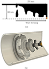 |
Figure 3. The optimized wave focusing SBH achieved in the computational design optimization study by Mousavi et al. [17]. Figure modified from Mousavi et al. [17]. (a) Axi-symmetrical model; (b) A 3D visualization |
In this study, we conduct a transient analysis of the optimized SBH (sonic black hole) achieved by Mousavi et al. [17] to answer the above mentioned questions. Although some important system properties like wave slowdown or dispersion are not straightforward to analyze in frequency domain, only rarely [24] has time domain analysis been used to study SBH behavior. In this paper, we develop a novel methodology to study wave slowdown in an SBH structure by the use of time domain information, and show in detail how the effective wave propagation speed and signal dispersion can be analyzed.
Our investigation uses two mathematical models, the lossless scalar acoustic wave equation as well as a viscothermal model, the linearized compressible flow equations. Following a concise overview of the governing equations in the second section, we detail the finite element (FE) discretization in the subsequent section. Here, we present the mesh discretization and geometry specifics of the optimized SBH. The behavior of the SBH is extensively examined in the final section of this study.
2 Governing equations
To investigate the optimized SBH introduced above, we use and compare both the lossless as well as the viscothermal acoustics formulations presented in detail by Hassanpour Guilvaiee et al. [48], Berggren et al. [49], Kampinga et al. [50]. Neglecting viscous and thermal losses, the governing equation is the lossless acoustic wave equation

where c0 is the speed of sound, pa the acoustic pressure, and Ωa the spatial region. As boundary conditions (BCs) we use the natural, homogeneous Neumann BC, i.e. a sound hard boundary, for the wall of the pipes Γwa and an inhomogeneous Dirichlet condition at the inlet Γin,


respectively, where pe(t) denotes the known excitation signal. Due to the small dimension of the SBH, the modeling of viscous and thermal losses is needed. Viscous and thermal effects can be accounted for by considering the linearized compressible flow equations. These so-called viscothermal equations result from the linearized conservation equations for mass, momentum, and energy combined with an equation of state. For an ideal gas with no background flow, the viscothermal equations read


where v and T denote the velocity and thermal fluctuations around zero and the ambient temperature, respectively, cp the heat capacity at constant pressure, and Ωvth the spatial domain. The stress tensor σ and the heat flux q are defined as

and
where γT is the thermal conductivity, and the bulk and dynamic viscosity are denoted by μB and μ, respectively. At the wall of the SBH, we enforce non-slip and isothermal boundary conditions, that is, the homogeneous Dirichlet conditions

In order to assess the importance of viscothermal losses, both models will be compared when analyzing the SBH design in the following.
Modeling with the viscothermal equations is computationally expensive, due to the need to solve for pressure, velocity, and temperature degrees of freedom, and the need to resolve the very thin boundary layers, which are smaller than the wavelength by a factor in the order of 10−5 to 10−3 in the audio regime. Therefore, these equations are only used where necessary, that is, in the actual SBH. In regions where viscous and thermal effects can be neglected, the lossless acoustic wave equation suffices. The coupling between these two models is performed by enforcing continuity of traction and velocity at the interface Γavth between the models, that is,


where n is the normal vector at the interface. A coupled formulation is obtained by inserting the coupling conditions into the boundary terms of the weak form, where accounting for the correct direction is important and can be implemented on non-conforming interfaces, as demonstrated by Hassanpour Guilvaiee et al. [51]. The finite element formulation of the above equation is presented in more details by Hassanpour Guilvaiee et al. [48] and implemented in the open-source finite element software openCFS [52].
3 Finite element computations of the sonic black hole
Finite element computations of the optimized SBH are performed using the open-source finite element software openCFS [52]. Figure 4 depicts the geometry, where we added input and output channels in addition to the main SBH domain. The simulations are performed in axisymmetric geometry with respect to the horizontal (y) axis. In this study, the input and output channels are modeled using the lossless acoustics formulation, while the SBH is modeled with the lossless as well as with the viscothermal acoustics formulation to explore the role of the viscous and thermal losses.
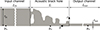 |
Figure 4. Geometry of the sonic black hole (SBH). Input and output channels are truncated in this figure. |
The input and output channels are assumed long enough to avoid reflections from the ends of the input and output channels to reach the SBH during the simulation time. The input and output channels are Lin=Lout= 20 m in length and the length of the SBH is L = 25.5 cm. The input rin and output rout radii of the input and output channels are 11.5 cm and 1.6 cm, respectively. To analyze the transient behavior of the SBH, a pressure wave packet excitation is applied on the left boundary of the entrance channel. Table 1 contains the material properties of air utilized in our simulations.
Air material properties.
Figure 5 depicts the mesh discretization used in this study. Inside the SBH, a quite fine mesh is required, in particular in the vicinity of the boundaries, where viscous and thermal boundary layers form. The required mesh size is governed by the smallest viscous boundary layer thickness corresponding to the highest frequency analyzed (1000 Hz), which is around 70 μm. Thus, we used an element size of 65.4 μm in the boundary layer, ensuring the velocity field in the thickness direction is approximated by at least three unknowns (of one quadratically interpolated element). In order to arrive at a mesh fitting to the broadband excitation signal, we coarsen the elements away from the boundary, thereby also accommodating the thicker boundary layers associated with the lowest frequencies contained in the excitation signal. The lowest frequencies (of about 10 Hz) also govern the necessary size of the viscothermal regions around the boundaries. A few boundary layer thicknesses should be considered to ensure a sufficient decay of the solution before the coupling to the lossless formulation is used. Since modelling errors can be expected if the coupling to the lossless formulation is done too early, we decided to model the entire internal geometry of the SBH with the viscothermal formulation. This also simplified the meshing of the complex-shaped SBH. In the input and output channels, a coarser mesh is sufficient due to the use of the lossless acoustics model in these regions. Note also the use of nonconforming meshes at the interface between the lossless and viscothermal models. The same mesh, containing exclusively hexahedral elements, is used for both the lossless and viscothermal computations.
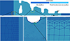 |
Figure 5. Mesh discretization of the sonic black hole. Finer mesh is dedicated to the boundaries to capture the viscous and thermal losses. |
The viscothermal region contains approximately 125 k elements (with second-order Ansatz functions for velocity and temperature, and first-order for pressure) and the in- and output pipes contain about 45 k elements (of first order) resulting in a total of about 1.2 M degrees of freedom in the linear system.
The numeric time integration is done with zero initial conditions for all fields using an implicit Crank–Nicolson scheme. For the two excitation signals illustrated in Figures 6 and 7, a time step size of 10 μs was used, and 10,500 steps were required to obtain a sufficient simulation time for the analysis.
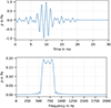 |
Figure 6. Excitation pressure signal with frequency content within the operational range of the SBH in time and frequency domain. |
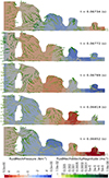 |
Figure 7. Excitation pressure signal with frequency content also outside the operational range of the SBH in time and frequency domain. |
For postprocessing purposes, three points, named p1, p2, and p3 in Figure 4, are positioned along the input channel, SBH and output channel at locations 6 m, 11.85 cm, and −85 cm, respectively.
4 Behavior of the optimized sonic black hole
As discussed in the introduction, the objective of the optimization was to obtain a device in which the wave power is focused at the outlet in the considered frequency interval. In this section, we aim to study, in time domain, the behavior of the optimized SBH, in terms of focusing behavior, reflection and transmission coefficients, dispersion characteristics, and effective wave propagation speed.
For this aim, we impose, at the inlet of the input channel, a truncated sinc pressure wave packet with a peak amplitude of 1 Pa and a central frequency of 700 Hz. The wave packet, depicted in time and frequency domain in Figure 6, persists for 20 ms.
The discrete Fourier transform (DFT) of the signal, indicates a frequency range approximately from 500 Hz to 800 Hz, corresponding to a longest wavelength of 69 cm. This frequency range is well within the range 400–1000 Hz for which the SBH was designed. It is also below the cut-off frequency of any higher-order wave propagation modes in the in- and output channels of 866 Hz and 6.22 kHz, respectively. Thus, only plane waves can propagate in the circular channels.
After approximately 60 ms, the input wave packet reaches the SBH. Figure 8 illustrates the pressure distribution inside the SBH at five different instants in time. Figure 8 illustrates the focusing aspect of the SBH, where the pressure amplitude is progressively increased as the wave moves through the device. The wave packet with the maximum amplitude of 1 Pa enters the SBH at 67.34 ms and leaves the SBH at 68.53 ms with an amplitude greater than 5 Pa. The velocity arrows plotted in Figure 8 depict the particle velocity orientations.
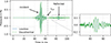 |
Figure 8. Pressure field inside the SBH. The velocity shown by green arrows demonstrates the particle movement. |
4.1 Reflection and transmission coefficients
In the transient simulation of this optimized SBH, the input and output channels are assumed to be sufficiently long so that no entrance or exit boundary reflections enter the domain of interest. Consequently, reflections solely originate from the SBH itself. Figure 9 illustrates the pressure time history at point p1, as depicted in Figure 4, in both the lossless and viscothermal cases. Point p1 is located 14 m from the excitation boundary and 5.745 m from the SBH. This means that the wave packet reaches p1 at approximately 40 ms and leaves it 20 ms later, as shown in Figure 9. Following the departure of the excitation wave packet, the reflected wave packet arrives at p1 at 70 ms, approximately 10 ms later.
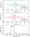 |
Figure 9. Pressure at point p1 located at the input channel. Incident pressure and reflected pressure are indicated in the figure. The separation time for calculating the reflection coefficient is denoted by tcut. |
This time delay facilitates the calculation of the reflection coefficient. In Figure 9, the separation time between the incident pressure wave and the reflected wave is denoted by tcut. The reflection energy coefficient R at a point such as p1 is defined as the ratio between the incident (total energy) and the reflected energy, calculated as
where the separation time and the total simulation time tend are set to 64 ms and 105 ms, respectively.
Figure 10 shows the transmitted wave packet at point p3. The pressure amplitude is significantly higher than the excitation pressure amplitude, indicating the energy-focusing aspect of the SBH. Naturally enough, the lossless acoustic model yields higher amplitudes than the viscothermal model, but only marginally so. Moreover, the propagation speed using the lossless model seems slightly faster than that for the viscothermal model.
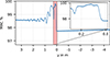 |
Figure 10. Pressure time signal inside the SBH at point p2 (top), transmitted pressure signal at p3 after the SBH (middle), and their respective frequency content (bottom). |
The energy transmission coefficient Tr is defined as the ratio between the energy that travels through the SBH, which can be observed at any location after the SBH, and the incident energy. This energy coefficient can be computed after the SBH at the output channel, for instance at point p3 (Fig. 4) as
For this wave packet, and using the reflection and transmission formulas (9) and (10), we obtain a reflection coefficient of 1.35%, and a transmission coefficient of 98.34% in the case of the lossless model. Some of the wave energy may still be trapped in the SBH, which can explain why the sum reaches 99.69%. In comparison, the viscothermal model yields a reflection coefficient of 1.42% and a transmission coefficient of 93.69%, indicating an absorption coefficient of approximately 4.5% due to viscothermal losses inside the SBH. The high transmission coefficient confirms that the SBH structure is an excellent focusing device (for the optimized frequency range). As only a small portion of wave energy is dissipated within the SBH, a reflective termination at the outlet would lead to large reflections. This is in contrast to the common rib-design SBH, where typically a large portion of wave energy is absorbed within the SBH.
4.2 Similarity of time history pressure signals
Figure 9 shows the time history of the pressure signals at the inlet of the SBH. In Figure 10 the pressure wave within and after the SBH is visualized. These plots indicate a high degree of similarity at different locations in the SBH and in the inlet and outlet channels, also indicated by the comparison of the frequency content of the signals. The consistency observed in the shape of these signals at various points along the SBH prompts a thorough investigation into their similarity.
To quantitatively measure the similarity of these signals, we employ the maximum of the time dependent Pearson correlation coefficient (PCC) between excitation signal pe(t) and computed pressure signal py(t) at each location y along the axis of the SBH. We first determine the time delay between the signals by searching for the argument of the maximum of the cross-correlation function, i.e. the time shift is

where * denotes the convolution, which was evaluated based on the time-discrete data. A normalized similarity measure is then given by the Modal Assurance Criterion (MAC) value [53] as
where
![$$ A =\bigl [p_e(t_1),p_e(t_2),\dots \bigr ], $$](/articles/aacus/full_html/2025/01/aacus240144/aacus240144-eq17.gif)
![$$ B_y =\bigl [p_y(t_1+\tau _y),p_y(t_2+\tau _y),\dots \bigr ], $$](/articles/aacus/full_html/2025/01/aacus240144/aacus240144-eq18.gif)
are row vectors containing the excitation and the time-shifted response at position y. The MAC value provides a robust evaluation of signal similarity, regardless of their amplitudes. It ranges between 0 and 1, where 0 indicates total dissimilarity and 1 signifies identical shapes. Since our signals are essentially mean-free, the MAC from (12a) corresponds to the absolute value of the PCC.
Figure 11 presents the MAC value along the input channel, SBH, and the output channel, using lossless acoustic wave equation (2). The MAC values range from 97.5% to almost 99.8% across these regions, indicating a high degree of signal similarity along the SBH, and thus a low degree of effective dispersion. At the input channel, where incident and reflected waves coexist, the MAC value was slightly lower compared to within the SBH. This decrease can be attributed to the presence of reflected waves. Within the SBH, the similarity of waves was more pronounced, indicating a higher MAC value, as the waves experienced partial reflection. However, as waves progressed towards the output channel, the similarity decreased due to the absence of the incident wave and partial reflection of waves.
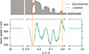 |
Figure 11. MAC value along the y-axis. A measure of similarity among the excitation signal and the time history pressure signals along the input channel, SBH and output channel. The pink region depicts inside the SBH. |
4.3 Effective wave propagation speed
As reviewed in the introduction, structural ABHs are designed with the aim of a gradual slowing of the propagation speed, which leads to a wave focusing effect. The conceptual ribbed design of an SBH first proposed by Mironov and Pislyakov [16] was designed based on the same idea, aiming for a gradual slowing of the effective axial propagation speed. Unfortunately, the ribbed design fails in practice to produce wave focusing due to the use of an unrealistic model of the wall admittance [38]. In contrast, the SBH investigated here was designed solely considering its wave focusing properties. As we show here, the SBH will nevertheless, as a byproduct, show a distinct slowing down of the average effective axial propagation speed.
To showcase this slow-down effect, we initially compute the average wave speed along the SBH. Based on the time history pressure signals at the inlet and outlet of the SBH, we find the instances when the incident wave packet (represented for instance by its peak) reaches the start of SBH, denoted Lin, and when it exits the SBH, located at Lin+L. By identifying these instances as tin and tout respectively, the averaged wave propagation speed is computed as cavg=L/(tout−tin).
Since the incident pressure is a continuous signal, determining the wave propagation speed solely based on the pressure peak may not provide the most precise results. Consequently, we decided to calculate the time difference by performing a cross-correlation as in (11), but with the pressure signals at Lin and Lin+L. The argument of the maximum value of the cross-correlation function is an accurate and robust estimation of the time shift.
The so computed average effective wave propagation speed within the SBH for the lossless acoustic model is 231.02 m s−1, while incorporating the viscothermal effect yields 228.90 m s−1. Thus, the average wave propagation speed in the SBH is significantly lower than the phase speed 342 m s−1, which is also the propagation speed in the waveguides. It is worth noting that both approaches, whether considering peak travel time or performing cross-correlation, yield comparable wave propagation speeds.
This result prompts the question of whether the wave packet gradually decelerates or maintains a constant lower speed along the SBH. To address these questions, we analyze the wave speed along the symmetry axis of the SBH. Instead of considering only two points, we opt for several points along the symmetry axis in the SBH, corresponding to the mesh nodes. For each axis point, we evaluate the time history pressure signals and cross-correlate them with the excitation signal to obtain the time shift according to (11), which, knowing the axis point locations, provides the speed profile.
Figure 12 shows the propagation wave speed profile calculated using this method, affirming the method's reliability by indicating a continuous, constant speed of 342 m s−1 in the channels outside the SBH, which equals the phase velocity. Figure 12 also illustrates the effective wave speed inside SBH, depicting fluctuations ranging approximately from 100 to 500 m s−1. Thus, in contrast to the structural ABH, the wave propagation speed is not monotonically slowed. A closer examination reveals that the effective local speed correlates with the local geometry. For each minimum in the cross-section profile there is a corresponding minimum in the effective wave speed profile, and for each chamber (cross-section maximum) there is a corresponding maximum in the effective wave speed. Thus waves approaching a minimum in cross-section seem to slow down while they accelerate once they enter into a larger cavity. The impact of the SBH onto the effective wave propagation speed actually extends about one pipe radius from the device. The special design of this optimized SBH makes it possible not only to decrease the average wave propagation speed to 230 m s−1 but also to locally increase the effective wave speed up to 500 m s−1.
 |
Figure 12. Effective wave speed profile using the cross-correlation method. |
4.4 SBH behavior beyond optimized frequency range
Our optimized SBH is designed for focusing the energy within a targeted frequency range of 400–1000 Hz. The threshold frequency depends on the length of the device; the longer the device, the lower the threshold frequency. To stay comfortably away from the presence of propagating higher radial modes, the upper limit of 1000 Hz was explicitly chosen as the highest frequency considered in the optimization. (The threshold frequency for propagation of the first non-planar axisymmetric mode is 1803 Hz.)
In this section, we extend our inquiry by subjecting the SBH to a wideband excitation signal, thereby exploring its behavior beyond the optimized frequency range. Figure 7 illustrates the time signal and frequency spectrum of the input excitation, encompassing the wider frequency range 50–1500 Hz. Note that, as in our previous study, the signal ends at 20 ms. All other simulation parameters, including geometry, remain consistent with those employed in the preceding investigation. Therefore, the simulation time, the separation time (tcut), and the pressure study points (p1 and p3) remain the same.
In line with our previous investigation, we can compute the transition and reflection coefficients. To illustrate the performance of the SBH across various frequencies, we perform a DFT of the pressure signals acquired at positions p1 and p3. Note that, for the reflection coefficient, we initially cut the pressure signal (at p1) at time t=tcut, after which we apply the DFT to obtain the spectrum of the reflection energy. Following this, the energy computation is conducted, incorporating both the inlet and outlet radii. Subsequently, we divide it by the DFT of the incident pressure signal, frequency per frequency, to determine the reflection and transmission coefficients.
Figure 13 presents these coefficients across various frequencies, utilizing both lossless and viscothermal acoustics formulations. As anticipated, within the optimized frequency range, the transmission coefficient approaches unity, while the reflection coefficient diminishes to nearly zero. However, beyond this range, there is a marked shift in these coefficients. Figure 13 illustrates a sharp increase in the reflection coefficient, nearing unity, implying that virtually all incident waves are reflected, empowering the SBH as a highly efficient bandpass filter.
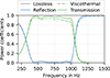 |
Figure 13. Reflection and transmission coefficients at various frequencies. Solid and dashed lines indicate lossless and viscothermal acoustics simulations, respectively. The coefficients are obtained by the DFT of the transient simulations. |
Moreover, Figure 13 depicts a (slight) difference between the lossless and viscothermal acoustic models. For the viscothermal model, owing to losses, the transmission coefficient exhibits a slight reduction compared to the reflection coefficient, a trend consistent with our earlier observations. Nonetheless, the differences between the reflection coefficients are modest. The coefficients computed from time domain data agree well with earlier results (Mousavi et al. [17], Fig. 9) obtained directly from frequency domain simulation.
Analyzing the similarity between the pressure time history at each point along the axis and the input time signal reveals that for the wideband excitation, the pulse shape is significantly altered. The MAC values were computed as described in Section 4.2 and are displayed in Figure 14 showing low similarity levels of around 65% before the SBH and 40% after the SBH compared to almost 100% for the optimized pulse (see Fig. 11). Since the SBH reflects parts of the input signal (outside the SBH's optimized frequency range), the signal is changed as it travels through the SBH, indicating dispersion.
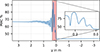 |
Figure 14. MAC value along the y-axis for the wideband excitation signal (depicted in Fig. 7). The pink region indicates values inside the SBH. |
5 Summary and conclusion
We have carried out a transient study of the optimized SBH introduced by Mousavi et al. [17]. This device works as a true wave focusing device by, on average, slowing down the acoustic waves and increasing the pressure amplitudes while producing low reflection and absorption coefficients within its operational frequency range of 400–1000 Hz. The simulation was performed using both a lossless and a viscothermal acoustics model, the latter modeling also includes the thermal and viscous losses inside the SBH. Applying to the inlet of the SBH a wave packet with a frequency content of about 500–800 Hz, the pressure amplitude increases by nearly seven times, while the reflection coefficient remains consistently below 1.5%. Moreover, the transmission energy rate is 93.69% when computed using the viscothermal acoustics model. Furthermore, our study showed that the averaged wave propagation speed in the SBH is reduced from 342 m s−1 to 230 m s−1. This wave speed reduction is not gradual and varies locally based on the shape of SBH. Interestingly, we observed that the pressure time history at various locations is consistent and similar to the excitation signal. To mathematically define this similarity, the MAC number is presented. Its value is higher than 98% along the SBH and in the input and output channels, indicating a low dispersion of the applied wave packet. The final section of our study shows that the SBH can also function as a band-pass filter, sharply reflecting back incoming frequency components outside its operational frequency range.
Acknowledgments
The authors would like to thank Emadeldeen Hassan for his help in providing the excitation sinc pressure signal, and Felix Huber for help with additional data analysis and visualisation during the review process.
Funding
This work was supported by the Swedish Research Council (Grant Nos. 2018-03546 and 2022-03783).
Conflicts of interest
The authors declare no conflict of interest.
Data availability statement
Data are available on request from the authors.
References
- A. Pelat, F. Gautier, S.C. Conlon, F. Semperlotti: The acoustic black hole: a review of theory and applications. Journal of Sound and Vibration 476 (2020) 115316. https://doi.org/10.1016/j.jsv.2020.115316 [CrossRef] [Google Scholar]
- M. Mironov: Propagation of a flexural wave in a plate whose thickness decreases smoothly to zero in a finite interval. Soviet Physics: Acoustics 34 (1988) 318–319 [Google Scholar]
- T. Weimann, A. Molter, L. Fernandez, M. He: Structural vibration control based on the effect of acoustic black holes and piezoelectric actuators. Finite Elements in Analysis and Design 224 (2023) 103992. https://doi.org/10.1016/j.finel.2023.103992 [CrossRef] [Google Scholar]
- J. Deng, X. Chen, Y. Yang, Z. Qin, W. Guo: Periodic additive acoustic black holes to absorb vibrations from plates. International Journal of Mechanical Sciences 267 (2024) 108990. https://doi.org/10.1016/j.ijmecsci.2024.108990 [CrossRef] [Google Scholar]
- Y. Xiao, W. Shen, H. Zhu, Y. Du: An acoustic black hole absorber for rail vibration suppression: Simulation and full-scale experiment. Engineering Structures 304 (2024) 117647. https://doi.org/10.1016/j.engstruct.2024.117647 [CrossRef] [Google Scholar]
- X. Chen, Y. Jing, J. Zhao, J. Deng, X. Cao, H. Pu, H. Cao, X. Huang, J. Luo: Tunable shunting periodic acoustic black holes for low-frequency and broadband vibration suppression. Journal of Sound and Vibration 580 (2024) 118384. https://doi.org/10.1016/j.jsv.2024.118384 [CrossRef] [Google Scholar]
- H. Li, O. Doaré, C. Touzé, A. Pelat, F. Gautier: Energy harvesting efficiency of unimorph piezoelectric acoustic black hole cantilever shunted by resistive and inductive circuits. International Journal of Solids and Structures 238 (2022) 111409. https://doi.org/10.1016/j.ijsolstr.2021.111409 [CrossRef] [Google Scholar]
- J. Deng, O. Guasch, L. Zheng, T. Song, Y. Cao: Semi-analytical model of an acoustic black hole piezoelectric bimorph cantilever for energy harvesting. Journal of Sound and Vibration 494 (2021) 115790. https://doi.org/10.1016/j.jsv.2020.115790 [CrossRef] [Google Scholar]
- W. Du, Z. Xiang, X. Qiu: Stochastic analysis of an acoustic black hole piezoelectric energy harvester under gaussian white noise excitation. Applied Mathematical Modelling 131 (2024) 22–32. https://doi.org/10.1016/j.apm.2024.04.015 [CrossRef] [Google Scholar]
- Z. Zhang, H. Wang, C. Yang, H. Sun, Y. Yuan: Vibration energy harvester based on bilateral periodic one-dimensional acoustic black hole. Applied Sciences 13 (2023) 6423. https://doi.org/10.3390/app13116423 [CrossRef] [Google Scholar]
- J. Zhao, Y. Huang, W. Yuan, J. Zhang, C. Song, X. Zhang, Y. Pan: Broadband acoustic black hole for wave focusing and weak signal sensing. Applied Acoustics 200 (2022) 109078. https://doi.org/10.1016/j.apacoust.2022.109078 [CrossRef] [Google Scholar]
- X. Wang, X. Liu, T. He, D. Xiao, Y. Shan: Structural damage acoustic emission information enhancement through acoustic black hole mechanism. Measurement 190 (2022) 110673. https://doi.org/10.1016/j.measurement.2021.110673 [CrossRef] [Google Scholar]
- J. Fu, T. He, Z. Liu, Y. Bao, X. Liu: A novel waveguide rod with acoustic black hole for acoustic emission signal enhancement and its performance. Ultrasonics 138 (2024) 107260. https://doi.org/10.1016/j.ultras.2024.107260 [CrossRef] [PubMed] [Google Scholar]
- L. Zhao, C. Bi, M. Yu: Structural lens for broadband triple focusing and three-beam splitting of flexural waves. International Journal of Mechanical Sciences 240 (2023) 107907. https://doi.org/10.1016/j.ijmecsci.2022.107907 [CrossRef] [Google Scholar]
- J. Deng, L. Zheng, O. Guasch: Elliptical acoustic black holes for flexural wave lensing in plates. Applied Acoustics 174 (2021) 107744. https://doi.org/10.1016/j.apacoust.2020.107744 [CrossRef] [Google Scholar]
- M. Mironov, V. Pislyakov: One-dimensional acoustic waves in retarding structures with propagation velocity tending to zero. Acoustical Physics 48 (2002) 347–352 [CrossRef] [Google Scholar]
- A. Mousavi, M. Berggren, L. Hägg, E. Wadbro: Topology optimization of a waveguide acoustic black hole for enhanced wave focusing. The Journal of the Acoustical Society of America 155 (2024) 742–756. https://doi.org/10.1121/10.0024470 [CrossRef] [PubMed] [Google Scholar]
- M. Mironov, V. Pislyakov: One-dimensional sonic black holes: Exact analytical solution and experiments. Journal of Sound and Vibration 473 (2020) 115223. https://doi.org/10.1016/j.jsv.2020.115223 [CrossRef] [Google Scholar]
- A.A. El Ouahabi, V.V. Krylov, D.J. O’Boy: Experimental investigation of the acoustic black hole for sound absorption in air, in the 22nd International Congress on Sound and Vibration (ICSV22), Florence, Italy, 12–16 July, 2015 [Google Scholar]
- X. Zhang, N. He, L. Cheng, X. Yu, L. Zhang, F. Hu: Sound absorption in sonic black holes: wave retarding effect with broadband cavity resonance. Applied Acoustics 221 (2024) 110007. https://doi.org/10.1016/j.apacoust.2024.110007 [CrossRef] [Google Scholar]
- M. Červenka, M. Bednařík: On the role of resonance and thermoviscous losses in an implementation of “acoustic black hole” for sound absorption in air. Wave Motion 114 (2022) 103039. https://doi.org/10.1016/j.wavemoti.2022.103039 [CrossRef] [Google Scholar]
- M. Červenka, M. Bednařík: Maximizing the absorbing performance of rectangular sonic black holes. Applied Sciences 14 (2024) 7766. https://doi.org/10.3390/app14177766 [CrossRef] [Google Scholar]
- J. Deng, O. Guasch, D. Ghilardi: Solution and analysis of a continuum model of sonic black hole for duct terminations. Applied Mathematical Modelling 129 (2024) 191–206. https://doi.org/10.1016/j.apm.2024.01.046 [CrossRef] [Google Scholar]
- S. Li, X. Yu, L. Cheng: Enhancing wave retarding and sound absorption performances in perforation-modulated sonic black hole structures. Journal of Sound and Vibration 596 (2025) 118765. https://doi.org/10.1016/j.jsv.2024.118765 [CrossRef] [Google Scholar]
- Q. Mao, L. Peng: Broadband and high-efficiency acoustic energy harvesting with loudspeaker enhanced by sonic black hole. Sensors and Actuators A: Physical 379 (2024) 115888. https://doi.org/10.1016/j.sna.2024.115888 [CrossRef] [Google Scholar]
- S. Li, J. Xia, X. Yu, X. Zhang, L. Cheng: A sonic black hole structure with perforated boundary for slow wave generation. Journal of Sound and Vibration 559 (2023) 117781. https://doi.org/10.1016/j.jsv.2023.117781 [CrossRef] [Google Scholar]
- X. Zhang, L. Cheng: Broadband and low frequency sound absorption by sonic black holes with micro-perforated boundaries. Journal of Sound and Vibration 512 (2021) 116401. https://doi.org/10.1016/j.jsv.2021.116401 [CrossRef] [Google Scholar]
- Y. Chen, K. Yu, Q. Fu, J. Zhang, X. Lu, X. Du, X. Sun: A broadband and low-frequency sound absorber of sonic black holes with multi-layered micro-perforated panels. Applied Acoustics 217 (2024) 109817. https://doi.org/10.1016/j.apacoust.2023.109817 [CrossRef] [Google Scholar]
- K. Petrover, A. Baz: Acoustic black hole with functionally graded perforated rings. Journal of Applied Physics 135 (2024) 234501. https://doi.org/10.1063/5.0216724 [CrossRef] [Google Scholar]
- Y. Chen, K. Yu, Q. Fu, J. Zhang, X. Lu: Modification of the transfer matrix method for the sonic black hole and broadening effective absorption band. Mechanical Systems and Signal Processing 220 (2024) 111660. https://doi.org/10.1016/j.ymssp.2024.111660 [CrossRef] [Google Scholar]
- L. Peng, Q. Mao: Helmholtz resonator with sonic black hole neck. International Journal of Acoustics and Vibration 28 (2023) 460–468. https://doi.org/10.20855/ijav.2023.28.42006 [CrossRef] [Google Scholar]
- Y. Ou, Y. Zhao: Design, analysis, and experimental validation of a sonic black hole structure for near-perfect broadband sound absorption. Applied Acoustics 225 (2024) 110196. https://doi.org/10.1016/j.apacoust.2024.110196 [CrossRef] [Google Scholar]
- T. Bravo, C. Maury: Broadband sound attenuation and absorption by duct silencers based on the acoustic black hole effect: Simulations and experiments. Journal of Sound and Vibration 561 (2023) 117825. https://doi.org/10.1016/j.jsv.2023.117825 [CrossRef] [Google Scholar]
- T. Bravo, C. Maury: Converging rainbow trapping silencers for broadband sound dissipation in a low-speed ducted flow. Journal of Sound and Vibration 589 (2024) 118524. https://doi.org/10.1016/j.jsv.2024.118524 [CrossRef] [Google Scholar]
- J. Deng, O. Guasch: Sound waves in continuum models of periodic sonic black holes. Mechanical Systems and Signal Processing 205 (2023) 110853. https://doi.org/10.1016/j.ymssp.2023.110853 [CrossRef] [Google Scholar]
- F. Bikmukhametov, L. Glazko, Y. Muravev, D. Pozdeev, E. Vasiliev, S. Krasikov, M. Krasikova: Ventilated noise-insulating metamaterials inspired by sonic black holes, 2024. https://doi.org/10.48550/ARXIV.2409.02731 [Google Scholar]
- Y. Li, L. Li, L. Xiao, L. Cheng, X. Yu: Enhancing ventilation window acoustics with sonic black hole integration: a performance evaluation. Applied Acoustics 229 (2025) 110388. https://doi.org/10.1016/j.apacoust.2024.110388 [CrossRef] [Google Scholar]
- A. Mousavi, M. Berggren, E. Wadbro: How the waveguide acoustic black hole works: A study of possible damping mechanisms. Journal of the Acoustical Society of America 151 (2022) 4279–4290. https://doi.org/10.1121/10.0011788 [CrossRef] [PubMed] [Google Scholar]
- O. Umnova, D. Brooke, P. Leclaire, T. Dupont: Multiple resonances in lossy acoustic black holes – theory and experiment. Journal of Sound and Vibration 543 (2023) 117377. https://doi.org/10.1016/j.jsv.2022.117377 [CrossRef] [Google Scholar]
- M. Berggren, A. Mousavi, L. Hägg, E. Wadbro: Topology optimization of wave-focusing waveguide acoustic black holes. Journal of the Acoustical Society of America 153 (2023) A70. https://doi.org/10.1121/10.0018195 [CrossRef] [Google Scholar]
- G. Serra, O. Guasch, M. Arnela, D. Miralles: Optimization of the profile and distribution of absorption material in sonic black holes. Mechanical Systems and Signal Processing 202 (2023) 110707. https://doi.org/10.1016/j.ymssp.2023.110707 [CrossRef] [Google Scholar]
- M. Červenka, M. Bednařík: Numerical study of the behavior of rectangular acoustic black holes for sound absorption in air. Wave Motion 123 (2023) 103230. https://doi.org/10.1016/j.wavemoti.2023.103230 [CrossRef] [Google Scholar]
- H. Sheng, M.-X. He, H. Pueh Lee, Q. Ding: Quasi-periodic sonic black hole with low-frequency acoustic and elastic bandgaps. Composite Structures 337 (2024) 118046. https://doi.org/10.1016/j.compstruct.2024.118046 [CrossRef] [Google Scholar]
- V. Hruška, J.-P. Groby, M. Bednařík: Complex frequency analysis and source of losses in rectangular sonic black holes. Journal of Sound and Vibration 571 (2024) 118107. https://doi.org/10.1016/j.jsv.2023.118107 [CrossRef] [Google Scholar]
- M. Bednařík, M. Červenka: A sonic black hole of a rectangular cross-section. Applied Mathematical Modelling 125 (2024) 529–543. https://doi.org/10.1016/j.apm.2023.09.005 [CrossRef] [Google Scholar]
- G. Bezancon, O. Doutres, O. Umnova, P. Leclaire, T. Dupont: Thin metamaterial using acoustic black hole profiles for broadband sound absorption. Applied Acoustics 216 (2024) 109744. https://doi.org/10.1016/j.apacoust.2023.109744 [CrossRef] [Google Scholar]
- A. Mousavi, M. Berggren, E. Wadbro: Extending material distribution topology optimization to boundary-effect-dominated problems with applications in viscothermal acoustics. Materials & Design 234 (2023) 112302. https://doi.org/10.1016/j.matdes.2023.112302 [CrossRef] [Google Scholar]
- H. Hassanpour Guilvaiee, P. Heyes, C. Novotny, M. Kaltenbacher, F. Toth: A validated modeling strategy for piezoelectric mems loudspeakers including viscous effects. Acta Acustica 7 (2023) 24. https://doi.org/10.1051/aacus/2023019 [CrossRef] [EDP Sciences] [Google Scholar]
- M. Berggren, A. Bernland, D. Noreland: Acoustic boundary layers as boundary conditions. Journal of Computational Physics 371 (2018) 633–650. https://doi.org/10.1016/j.jcp.2018.06.005 [CrossRef] [Google Scholar]
- W.R. Kampinga, Y.H. Wijnant, A. de Boer: A finite element for viscothermal wave propagation. 23rd International Conference on Noise and Vibration Engineering 2008 (ISMA 2008) 7 (2008) 4271–4278 [Google Scholar]
- H. Hassanpour Guilvaiee, F. Toth, M. Kaltenbacher: A non-conforming finite element formulation for modeling compressible viscous fluid and flexible solid interaction. International Journal for Numerical Methods in Engineering 123 (2022) 6127–6147. https://doi.org/10.1002/nme.7106 [CrossRef] [Google Scholar]
- M. Kaltenbacher, F. Toth, H. Hassanpour Guilvaiee: openCFS (coupled field simulation): a finite element-based multi-physics modelling and simulation tool. Available at https://openCFS.org/ (accessed April 3, 2025) [Google Scholar]
- S. Greś, M. Döhler, L. Mevel: Uncertainty quantification of the modal assurance criterion in operational modal analysis. Mechanical Systems and Signal Processing 152 (2021) 107457. https://doi.org/10.1016/j.ymssp.2020.107457 [CrossRef] [Google Scholar]
Cite this article as: Hassanpour Guilvaiee H. Mousavi A. Berggren M. Wadbro E, Kaltenbacher M, & Toth F. 2025. Transient study of an optimized waveguide sonic black hole with wave focusing properties 9, 36. https://doi.org/10.1051/aacus/2025019.
All Tables
All Figures
|
Figure 1. The ribbed design of a sonic black hole proposed by Mironov and Pislyakov [16] with an intention to create a wave focusing effect towards the end of the waveguide. Figure modified from Mousavi et al. [17]. (a) Axi-symmetrical model; (b) A 3D visualization |
| In the text | |
|
Figure 2. The conceptual setup for the design optimization problem. A plane wave enters Γin, and the problem is to place solid material Ωs in the region illustrated with a grid so that the acoustic power is maximized in the target region ΓT. Figure modified from Mousavi et al. [17]. |
| In the text | |
|
Figure 3. The optimized wave focusing SBH achieved in the computational design optimization study by Mousavi et al. [17]. Figure modified from Mousavi et al. [17]. (a) Axi-symmetrical model; (b) A 3D visualization |
| In the text | |
|
Figure 4. Geometry of the sonic black hole (SBH). Input and output channels are truncated in this figure. |
| In the text | |
|
Figure 5. Mesh discretization of the sonic black hole. Finer mesh is dedicated to the boundaries to capture the viscous and thermal losses. |
| In the text | |
|
Figure 6. Excitation pressure signal with frequency content within the operational range of the SBH in time and frequency domain. |
| In the text | |
|
Figure 7. Excitation pressure signal with frequency content also outside the operational range of the SBH in time and frequency domain. |
| In the text | |
|
Figure 8. Pressure field inside the SBH. The velocity shown by green arrows demonstrates the particle movement. |
| In the text | |
|
Figure 9. Pressure at point p1 located at the input channel. Incident pressure and reflected pressure are indicated in the figure. The separation time for calculating the reflection coefficient is denoted by tcut. |
| In the text | |
|
Figure 10. Pressure time signal inside the SBH at point p2 (top), transmitted pressure signal at p3 after the SBH (middle), and their respective frequency content (bottom). |
| In the text | |
|
Figure 11. MAC value along the y-axis. A measure of similarity among the excitation signal and the time history pressure signals along the input channel, SBH and output channel. The pink region depicts inside the SBH. |
| In the text | |
|
Figure 12. Effective wave speed profile using the cross-correlation method. |
| In the text | |
|
Figure 13. Reflection and transmission coefficients at various frequencies. Solid and dashed lines indicate lossless and viscothermal acoustics simulations, respectively. The coefficients are obtained by the DFT of the transient simulations. |
| In the text | |
|
Figure 14. MAC value along the y-axis for the wideband excitation signal (depicted in Fig. 7). The pink region indicates values inside the SBH. |
| In the text | |
Current usage metrics show cumulative count of Article Views (full-text article views including HTML views, PDF and ePub downloads, according to the available data) and Abstracts Views on Vision4Press platform.
Data correspond to usage on the plateform after 2015. The current usage metrics is available 48-96 hours after online publication and is updated daily on week days.
Initial download of the metrics may take a while.