| Issue |
Acta Acust.
Volume 9, 2025
|
|
|---|---|---|
| Article Number | 33 | |
| Number of page(s) | 16 | |
| Section | Virtual Acoustics | |
| DOI | https://doi.org/10.1051/aacus/2025018 | |
| Published online | 03 June 2025 | |
Scientific Article
Diffuse sound field synthesis: Towards practical source layouts
Institute of Electronic Music and Acoustics, University of Music and Performing Arts, 8010 Graz, Austria
* Corresponding author: This email address is being protected from spambots. You need JavaScript enabled to view it.
Received:
11
October
2024
Accepted:
22
April
2025
Abstract
In an ideal isotropic diffuse sound field, uncorrelated plane waves arrive uniformly from all directions. Recent theoretical work has shown that uncorrelated sources arranged on a spherical surface can also be used to synthesize diffuse fields that exhibit a uniformly vanishing active sound intensity, albeit without position-independent isotropy. How the principles extend to finite-sized rectangular cuboid and discrete source layouts remains an open question. This study considers the multi-axial superellipsoid as a flexible parametric geometry for uncorrelated acoustic source distributions. By tuning its shape parameter p, the superellipsoid transitions from an ellipsoid p=2 to a rectangular cuboid p→∞, enabling a systematic analysis of active intensity using differential geometry, Gegenbauer expansion, and numerical simulations. Findings indicate that a superellipsoidal source layer of directionally uniform density requires to be driven by a non-uniform source variance, for which a generic solution is proposed. For the ellipsoid, the proposed variance is exact and emphasizes distant sources, while for the rectangular cuboid, it remains an approximation, but still effectively emphasizes sources near edges and corners. For discrete source layouts, zero active intensity can be approximately synthesized within a domain shrunk by a factor of N/(N+1) provided that (i) sources are arranged in uniform directions of a tight spherical 2N+1 design and sample the proposed variance, or (ii) a comparable number of sources with uniform variance is distributed in a minimum potential energy configuration.
Key words: Sound field synthesis / Thomson problem / superellipsoid / spherical t-design
© The Author(s), Published by EDP Sciences, 2025
 This is an Open Access article distributed under the terms of the Creative Commons Attribution License (https://creativecommons.org/licenses/by/4.0), which permits unrestricted use, distribution, and reproduction in any medium, provided the original work is properly cited.
1 Introduction
The spherically isotropic diffuse field is a common concept of an ideal sound field, in which uncorrelated plane waves arrive from all directions with cylindrically or spherically isotropic variance, yielding a position-independent sound pressure level, a vanishing active sound intensity, and correlation that only depends on the Euclidean distance between two sound pressure observations [1].
Typical models of reverberation and the diffuse sound field in room acoustics can be found, e.g., in Kuttruff's textbook [2]. Advanced statistical theories considering diffuse fields were described by Polack [3] and Badeau [4], and for less ideal diffuse fields, anisotropy in reverberation was described by Nolan et al. [5]. Similarly, direction-dependent reverberation curves were observed by Berzborn and Vorländer [6], and common-slope modeling of multi-slope reverberation curves was proposed by Götz et al. [7]. Direction-dependent reverberation times were artificially generated by Alary et al. [8] and proven to exist, e.g., by Bilbao and Alary [9] for ideal rectangular cuboid rooms.
The synthesis of perfectly diffuse sound fields is essential for controlled laboratory conditions, enabling precise evaluation of various acoustic phenomena. This includes assessing the diffuse-field sound transmission of building partitions [10] and acoustic absorbers [11, 12], as well as analyzing the diffuse-field response of microphone arrays [13–15] and dummy heads [16–18]. Additionally, it plays a crucial role in evaluating the performance and perceptual quality of active noise control and cancellation algorithms [19–21]. Beyond measurement applications, diffuse sound field synthesis is also a key objective in spatial sound reproduction, where the goal is to create a perfectly enveloping auditory experience [22–26].
Basic spatial audio rendering techniques can effectively synthesize diffuse sound fields for moderately dense loudspeaker layouts and a centered listener [22]. For instance, object-based rendering with amplitude panning, channel-based rendering, or scene-based Ambisonic rendering could be considered. However when employed with point-source loudspeakers arranged in a circle (2D), inherent limitations become evident at off-center listening positions, according to recent studies that have shown there being limits of the synthesis region, in which a uniformly diffuse envelopment is perceived [25, 27–29]. Experimental results on 2D loudspeaker arrangements from [25, 30] suggest that circular arrangements of surrounding vertical line sources can extend the perceptually diffuse synthesis region.
For a more comprehensive introduction to diffuse-field synthesis with uncorrelated sources, readers are referred to recent theoretical studies: the theory by Tanaka and Otani on continuous- and discrete-direction uncorrelated plane waves [31–33], and our theory on continuous layers of surrounding sources at finite radius [34].
According to our theoretical work [34], continuous, uncorrelated layers of sources driven by a uniform variance σ2=1 can ideally and uniformly suppress the synthesis of active sound intensity, when arranged in the free field. Ideal layers include parallel, cylindrical, or spherical geometries, and require acoustic sources that correspond to Helmholtz Green's functions G(r) for the correct number D of space dimensions, see Table 1. In this framework, the expected active sound intensity was shown to exactly correspond to a surface integral over the variance times the gradient of the Green's function for the Laplace equation, denoted by the calligraphic symbol  , see Table 2. This follows from the relation
  . The underlying mathematical functions, rooted in potential theory, provide an analogy to Newton's spherical shell theorem in gravitational physics [35] and Gauß’ law in electromagnetism.
Green's function G(r) of the Helmholtz equation in D=1, 2, 3 space dimensions.
Green's function  of the potential equation in D=1, 2, 3 space dimensions and their derivative.
While this may be useful in theory, practical loudspeaker layouts in anechoic environments–even when employing the correct acoustic source type–rarely conform to idealized circular or spherical continuous layers. In many cases, spatial constraints require non-circular or non-spherical layouts, extended more in one dimension than others, or rectangular and cuboid geometries. Moreover, real-world synthesis relies on a finite number of discrete sources, making discretization strategies essential.
The theory by Tanaka and Otani [31–33] investigates how diffuse sound fields are synthesized under three different conditions: (i) an ideal of infinitely many uncorrelated plane waves, (ii) infinitely many plane waves controlled by a finite set of uncorrelated spherical harmonics, or (iii) a finite set of plane-wave directions laid out as spherical t-design [36] and driven by a finite set of uncorrelated spherical harmonics. For the imperfect cases (ii) and (iii), the authors introduce the term pseudo-perfect diffuseness. Differences were analyzed with regard to the isotropy metric by Nolan et al. [5] and other common diffuse-field metrics, such as two-point correlation and uniformity of the sound pressure level [37]. The reproduction of ideal metrics has been shown to be achievable within a region limited by the Helmholtz number kx<N, where x is the observer's distance from the origin, and k is the wave number. This limit holds when restricting the spherical harmonic order to N, using a spherical t=2N design, or both [32].
Despite the undeniable relevance of the kx<N limit for the set of investigated metrics–and its compliance with the limit for Ambisonic sound field synthesis at a given Ambisonic order N, cf. [38–44]–psychoacoustic studies suggest that a perceptually faithful synthesis is feasible under less restrictive constraints [45–47]. Given the psychoacoustic evidence and the frequency independence of active sound intensity in our theory [34], an alternative, less restrictive, and frequency-independent radial limit should be identified.
Listener envelopment, a key perceptual attribute of a diffuse sound field, depends on both low interaural level differences (ILDs) and low interaural coherence. Of these two metrics, studies of practical scenarios indicate that achieving sufficiently low interaural coherence is rarely a challenge [25, 29]. However, maintaining low ILDs has been shown to be challenging [25, 29]. ILDs arise due to acoustic shadowing by the listener's head and they should be proportional to the active sound intensity component along the interaural axis, normalized by the sound level, as assumed in Merimaa's work [48, 49]. As a simplification, the diffuseness metric ψ=1−∥I∥/(2cw) was introduced to quantify the absence of normalized active intensity [48, 49]. If a stronger empirical relationship between ILD and diffuseness ψ can be established, high diffuseness could be interpreted as eliminating directional bias indicated by perceptible ILDs, in the most sensitive head orientations. This may prove to be a perceptually relevant aspect of diffuse sound field synthesis.
To achieve a high diffuseness ψ with non-spherical or non-circular source layers, this paper focuses on an optimum source activation variance σ2, which needs not be constant but should minimize the synthesized active intensity, ideally reaching I=0. Apart from the relation to gravitation [34], the problem also relates to known problems in electrostatics. In a charged conductor, many electric charge particles distribute across its surface according to a continuous surface charge density σS ensuring that the internal electric field E=0 vanishes. Alternatively, if there is only a finite number of charges, their discrete positions will minimize the electric field inside the conductor. Existing studies on analytic surface charge density for multi-axial ellipsoidal conductors [50–52] provide valuable insights. However, for more arbitrary conductor shapes [53–55], numerical methods are the preferred approach [56, 57]. For a finite number of discrete sources, the problem closely relates to the Thomson problem, which seeks the optimal minimum-energy distribution of equally charged, mutually repelling electrons on a sphere, or more arbitrary surfaces [58–61]. This paper aims to refine and further exploit these analogies for the synthesis of diffuse sound fields.
1.1 Definitions and metrics
As previously investigated [34], common metrics can be employed such as active sound intensity I, potential sound energy density w, and diffuseness ψ in the sound field, cf. [2, 48, 49, 62, 63], as well as sectoral intensity  at the origin to monitor isotropy of I. These squared metrics include integrals of a source term, for which either
  or
or  remains after statistical expectation with uncorrelated acoustic sources, over the squared source density σ2(xs), as derived in [34]. The individual source at xs has the distance r=∥xs−x∥ from the observer at x along the direction
  , or r0=∥xs∥ from the origin along the direction
  , see Figure 1. At a source xs, the angle ϕ is the inclination between the direction vector u from the origin to the surface element dS(xs) whose normal is n, so that cosϕ=u⊺n. The surface element dS can be re-expressed as solid-angle element dΩ0 from the origin or dΩ from the observer
  , see Figure 1 and [34].
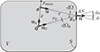 |
Figure 1. Rounded cuboid S enclosing V, locations: orig. 0, src. xs, rec. x, directions: u0, u, ux, n, distances: r0, x, xmax, r, elements/angles: dS, dΩ0, dΩ, ϕ0, ϕ. |
For any star-shaped, uncorrelated, continuous layer, this study considers sources distributed with uniform angular density within the solid angle dΩ0 for any direction u0 from 0, cf. Figure 1. Note that this is in contrast to our previous work [34], in which sources were distributed uniformly on the surface and got activated by a surface density σ2(xs), denoted as σS(xs) in equation (20), for distinction. For this study, sources shall be activated by a directional density σ2(u0) with regard to the origin, so that their contributions become  to the active sound intensity and
  to the potential sound energy density. These contributions define the integrals and the diffuseness metric ψ,
 (1)
(1)
 (2)
(2)
 (3)
(3)
These metrics can be evaluated at any observer position x. Discrete sources xsl=r0l u0l distributed uniformly across the directions use a sum over the index l, instead:
 (4)
(4)
 (5)
(5)
In both the continuous and discrete scenarios, the scalars N or  are used to equalize potential sound energy density at the center 2 ρ c2 w(0)=1, and physical quantities are density of air
  and speed of sound
  . In a diffuse sound field, these above metrics are expected to be
 (6)
(6)
while in the free sound field of a single source, the diffuseness metric vanishes ψ=0.
For the continuous layer equation (1) and a dedicated observer position x, we assume that every direction u observed relates to a position xs on the source layer S contributing
 (7)
(7)
to −ρ c I. Using  , the sectoral intensity observed within a small, differential cone dΩ around the observed direction u can be defined as:
 (8)
(8)
1.2 Condition for isotropy at x=0
As discussed in [34] and obvious from equation (8), a position-specific isotropic active intensity can be enforced and leads to an optimal source activation for the particular observer position x
 (9)
(9)
Similarly as shown in Figure 5 in [34], pervasive isotropy at every observer position is, however, infeasible unless both of the angles match ϕ=ϕ0. This match only happens either for an infinite sphere r0→∞, or at the origin x=0, where isotropy is enforced by
 (10)
(10)
1.3 Estimating perceptually relevant aspects
Regarding the technical metrics discussed above, it is important to estimate their perceptual relevance. For instance, non-ideal and non-continuous source layouts are expected to produce slightly lower diffuseness values than the ideal ψ<100%. A useful question is how much lower can ψ be before the imperfection becomes perceptible. The perceptual significance of the other metrics should also be addressed. Interestingly, not even ideal continuous source layers of finite radius are able to produce a perfectly constant sound energy density w≠const., perfect and position-independent isotropy  , or a two-point correlation of the sound pressure C(x, x+Δx, k)≠C(kΔx) that is independent of location and orientation, as shown in [34].
To maintain a reasonably constant sound pressure level or w, simulations shown in [30] suggest that shrinking the usable listening area to about 80% of the available dimensions keeps the level sufficiently constant, with variation on position change limited to 1 dB, which appears to be within the relevant JND of loudness [64, 65].
Sectoral intensity  exhibits strong directional variation when there is anisotropy, such as in the sparse circular configuration of uncorrelated vertical line sources simulated in [25, 29]. However, in large portions of these simulated fields, perceptual metrics, such as ILD and IC, exhibited only moderate variations. This suggests that fine-grained directional details of sectoral intensity may not be perceptually relevant. Moreover, since IC is derived from correlation, and interaural cross-correlation can be modeled by the two-point correlation in the sound field (Fig. 3 in [66]), the relative ease of achieving low IC suggests that precisely replicating the ideal isotropic two-point correlation function C(kΔx) may not be perceptually relevant.
The diffuseness ψ=1−∥I∥/(2c w) is arguably a macroscopic metric but reflects a fundamental acoustic cause of ILD [49, 67], and in case of uncorrelated sources also relates to IC. This is because ∥I∥ describes an overall balance in sectoral intensity. Depending on the relative contribution of active intensity  aligned with the interaural axis uia, a listener's head casts an acoustic shadow, yielding ILD. Accordingly, we propose modeling ILD–and for the synthesis with uncorrelated sources also IC–as inversely proportional to the diffuseness metric ψ.
To obtain a quantitative overview in relation to known perceptual thresholds [25, 68–70], we propose a simple model consisting of: (i) an isotropic diffuse sound field with a total plane-wave variance  , which mixes with (ii) a single direction of the variance
  . This model allows us to determine ILD and IC values resulting from the simple diffuse-plus-directional mixture for any given balance controlled by the diffuseness parameter ψ, as shown in Figure 2. The interaural cues were computed for different mixtures 0%≤ψ≤100% of uncorrelated diffuse sound and direct sound, the diffuse field was modeled either as horizontal (D=2) or spherical (D=3) surround layout, and the directional sound incidence was varied in angle across the frontal semi-circle. Binaural cues were simulated using the Neumann KU100 HRTFs [71] and averaged across gammatone frequency bands of one equivalent rectangular bandwidth (ERB), between 200 Hz and 12.8 kHz, using the models from previous works [25, 29]. The resulting curves in Figure 2 serve as a quantitative rule of thumb, summarizing how the diffuseness metric maps to noticeable interaural metrics [25, 29]:
-
–
The IC JND of 0.5 is generally uncritical and remains below threshold across directions with a diffuseness of ψ>40% as shown in Figure 2 (left).
-
–
In contrast, the ILD JND of approximately 1 dB is identified as the more critical cue, as depicted in Figure 2 (right). To render ILD perceptually irrelevant, a diffuseness as high as ψ>80%–90% is required when the directional component aligns with the interaural axis. No ILD is introduced if its direction lies in the median plane, making the IC the dominant cue in this region, requiring ψ>40%, as in the point above.
This motivates the explicit goal of this study: to synthesize a sound field with I→0 or ψ→100%. Simulations presented below include the ψ=90% contour as a reference for critical listening with sensitive head orientations.
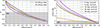 |
Figure 2. Interaural coherence (IC) and interaural level difference (ILD) evaluated for sound fields of varied diffuseness 0≤ψ≤1. The evaluation uses a variably-weighted mix of a 2D/3D diffuse sound field with a single plane wave from a horizontal, frontal azimuth angle. Gray areas indicate one just-noticeable difference (JND) from a diffuse-field reference with IC =0, ILD =0. |
2 Continuous superellipsoid layer
As a prototypical, practical definition of a layer shape S that contains all the source points xs=[xs1, …, xsD]⊺ and stays within the given bounds, we define a multi-axial superellipsoid [57, 72, 73] with the uniform exponent p,
 (11)
(11)
Its semi-axes a1, …, aD can be adjusted to fit spatial positions x=[x1, …, xD]⊺ in  restricted within rectangular bounds −ai≤xi≤ai of a room, for all Cartesian dimensions i=1, …, D. For p=2, S forms a multi-axial ellipsoid that touches the Cartesian boundaries only at its vertices and co-vertices. As p→∞, S approaches a rectangular cuboid, with sharp edges and corners fully occupying the available space. At an intermediate value, such as p=10, the edges and corners remain rounded, as shown in Figure 7 and resembling the sketch in Figure 1.
From the implicit definition  of the superellipsoid, cf. (11), the surface normal n is determined by the gradient [74, 75]
  ,
,
![Mathematical equation: $ $\boldsymbol n =\frac {\left [{{\mathsf{p}}}\,\frac {|x_{{\textrm {s}}i}|^{{{\mathsf{p}}}-1}}{a_i^{{\mathsf{p}}}}\right ]_i}{\sqrt {\sum _{i=1}^D\left ({{\mathsf{p}}}\,\frac {|x_{{\textrm {s}}i}|^{{{\mathsf{p}}}-1}}{a_i^{{\mathsf{p}}}}\right )^2}},$ $](/articles/aacus/full_html/2025/01/aacus240123/aacus240123-eq47.gif) (12)
(12)
and it plays an important role in the calculations below. Its inner product with its coordinate xs simplifies because of the definition  into
into
 (13)
(13)
2.1 Condition for vanishing active intensity with p=2
Newton demonstrated for gravitation inside a spherical shell [35], and Thomson and others later extended this to the equivalent ellipsoidal shell problem in electrostatics [50–52], that an enclosed region with a vanishing gradient field at any x∈V requires for any direction u an opposing-direction criterion that equivalently applies to diffuseness synthesis, cf. [34]:
 (14)
(14)
Applying this constraint to two surface positions xsl and xsm of the superellipsoid, with their variances  and
and  , equation (8) in Section 1.1 yields
 (15)
(15)
The cosines  and
and  involve unit vectors defined as
  and
and  , as well as the surface normal defined in equation (12). By these definitions, we obtain from the respective surface normals nl at xsl and nm at xsm:
 (16)
(16)
The observer position x can be freely chosen along the line between both positions  , which allows to cancel rij
 (17)
(17)
Inserting the inner product equation (13) for  and equation (12) for
  yields
 (18)
(18)
For p=2, the term ![Mathematical equation: $[1-\sum _{i=1}^D\frac {x_{{\textrm {s}}mi}x_{{\textrm {s}}li}}{a_i^2}]^{-1}$](/articles/aacus/full_html/2025/01/aacus240123/aacus240123-eq64.gif) equals on both sides and cancels. The resulting equation leads to the directional source activation for the ellipsoid that provides vanishing active intensity:
equals on both sides and cancels. The resulting equation leads to the directional source activation for the ellipsoid that provides vanishing active intensity:
 (19)
(19)
This directional density  with regard to the origin relates to the typical electrostatic surface charge density σS when inserted into the relation σS dS=σ2 dΩ0 between the corresponding integrals. Replacing
  , we can prove its equivalence, cf. equation (13),
 (20)
(20)
to the well-known expression for σS from analogous literature on electrostatics [50–52].
2.2 Proposal for small active intensity with p>1
For other p≠2, it is obvious that the factors ![Mathematical equation: $\Bigl [1-\sum _{i=1}^D\frac {x_{{\textrm {s}}li}x_{{\textrm {s}}li}^{{{\mathsf{p}}}-1}}{a_i^{{\mathsf{p}}}}\Bigr ]^{-1}$](/articles/aacus/full_html/2025/01/aacus240123/aacus240123-eq69.gif) and
and ![Mathematical equation: $\Bigl [1-\sum _{i=1}^D\frac {x_{{\textrm {s}}mi}x_{{\textrm {s}}li}^{{{\mathsf{p}}}-1}}{a_i^{{\mathsf{p}}}}\Bigr ]^{-1}$](/articles/aacus/full_html/2025/01/aacus240123/aacus240123-eq70.gif) on both sides of equation (18) are generally unequal in their dependency on i and j. They cannot be canceled, and the opposing direction criterion becomes useless for other values of p than 2. Using the boundary element methods [56] or round-robin cases in [57, 76, 77] could offer accurate but also effortful solutions. As a practical alternative, this paper proposes the approximate solution1 involving equation (19)
on both sides of equation (18) are generally unequal in their dependency on i and j. They cannot be canceled, and the opposing direction criterion becomes useless for other values of p than 2. Using the boundary element methods [56] or round-robin cases in [57, 76, 77] could offer accurate but also effortful solutions. As a practical alternative, this paper proposes the approximate solution1 involving equation (19)
 (21)
(21)
It is approximate for p≠2 but turns out to be accurate enough for the application, as demonstrated below.
3 Simulation study
3.1 Ellipse (D=2)
For D=2, Figure 3 analyzes the diffuseness and sound energy density of a 3:2 horizontal ellipse of vertical line sources (a–c). Obviously, the unity variance σ2=1 in (a) is not ideal for extended diffuseness greater than 90%; yet the diffuseness level already reaches a high level with >80% everywhere inside.
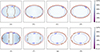 |
Figure 3. Diffuseness ψ (colormap, solid contour: 90%) and level w normalized to origin (dotted 1 dB contour) for 2D, 3:2 ellipse of 100 equi-angle uncorrelated vertical line sources (a–d) or 6:4:3 ellipsoid of 2500 maximum determinant nodes with uncorrelated point sources (e–h): (a, e) with unity variance σ2=1, (b, f) isotropy-enforcing variance |


The variance  in (b) greatly enlarges the 90% contour, and finally
  in (c) provides ideal diffuseness everywhere inside;
  in (d) is equivalent and therefore delivers the same result as (c); the potential sound energy density w is similar for all (a–d).
Figure 4 analyzes isotropy by the directional contributions observed at 0. For the ellipse of the ratio a1:a2=2:3, the distant sources are under-represented by the factor  , i.e. −1.76 dB, with unity variance, see ell σ2=1 curve. The ideal isotropy variance
  perfectly removes this shortcoming in the ell σ2=r0 curve, while the ideal diffuseness variance
  is not isotropic for the elliptical geometry, see ell
  curve. It overemphasizes distant sources and exaggerates their level by the factor
  , i.e. 1.76 dB.
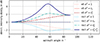 |
Figure 4. Directional intensity dI/dΩ0=σ2/r0 in 2D, normalized at 0°, observed at x=0 for different azimuth angles to between 0° and 90° (quadrants are symmetric) for 2:3 2D horizontal ellipse/rectangle of uncorrelated vertical line sources (superellipse p=10) with different variances σ2; isotropy requires σ2=r0. |
3.2 Rectangle/Superellipse (D=2)
The 3:2 horizontal p=10 superellipse with uncorrelated vertical line sources approximates a 3:2 rectangle and is analyzed Figures 5 (a–d) in terms of diffuseness synthesized by the directional variances (a) σ2=1, (b)  , (c)
, (c)  , and (d)
  . Ideal isotropy variance
  in (b) produces diffuseness inside that already exceeds 70%; the sound energy density levels w shown in the figure remain largely unaffected (a–c). Regarding the 90% diffuseness contour, isotropy variance
  in (b) greatly enlarges this contour, slightly more so does
  in (c), but it only reaches the corners for the simulation with the proposed superellipse approximation
  (d); the sound energy density levels w behave similarly for (e–h) as for the elliptic cases (a–d).
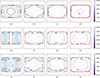 |
Figure 5. Diffuseness ψ (colormap, solid contour: 90%) and level w normalized to origin (dotted 1 dB contour), for the rectangle of the ratio 3:2 (2D), and for the cuboid of the ratio 6:4:3 (3D), both with p=10, using 100 equi-angular nodes as uncorrelated line vertical sources (2D) or 2500 maximum determinant nodes as uncorrelated point sources (3D), respectively: (e, i) with unity gain σ2=1,(f, j) isotropy-enforcing gain |


Figures 4 analyzes isotropy by the corresponding directional contributions, see rect curves. The noticeable difference to the ell curves of the ellipse occurs around the 56° angle targeting the corner of the circumscribed 3:2 rectangle. There, the maximum radius maxr0 is reached, σ2=1 exhibits a minimum directional contribution,  a maximum one, while
  is the ideal isotropy solution. The largest maximum and anisotropy is reached by the proposed approximation
  . Its curve indicates an over-emphasis of the contributions in the corners of up to 4.5 dB.
3.3 Ellipsoid (D=3)
For D=3, Figures 3 shows in (e–g) a similar analysis for an ellipsoid with the axis ratio 6:4:3. The cases in (e–g) are convincing already from (f) on and perfect in (g) and (h). The potential sound energy density w would nearly be perfectly flat for the gain σ2=1 in (e) compared to (f–h), but its diffuseness is only slightly higher than 70%, off center. In the (f–h) cases, slightly more than a +1 dB sound energy gain has to be accepted as unevenness near the boundaries. The proposed approximation  in (h) is identical to the accurate ellipsoid solution in (g).
Figures 6 analyzes the isotropy for the ellipsoid in (a–d) by the directional contributions for different choices of σ2. The isotropy-enforcing levels  accomplish perfectly flat results in (b), while for σ2=1 the most distant direction is quieter by about −6 dB in (a), and in (c)
  , it is louder by 4 dB. Isotropy in (d) of course matches with the equivalent solution (c).
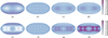 |
Figure 6. Directional intensity |

3.4 Cuboid/Superellipsoid (D=3)
The p=10 superellipsoid approximating a rectangular cuboid with the axes ratio 6:4:3 is analyzed in Figures 5 (e–l). The xy cross-section (e–h) only cuts the vertical edges, which seem to be uncritical compared to the 2D case above. The diagrams (f–h) already look convincing. For instance,  in (g) appears to be a good choice, and
  in (h) does not yield further improvements on the xy cut1. However, for the maps Figures 5 (i–l) of the inclined cross-section cut2, which runs through corners and edges of the superellipsoid as illustrated in Figures 7, the 90% contour of the analytic solutions Figures 5 (i–k) does not reach corners and edges, and it only does so with the proposed approximation (l).
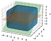 |
Figure 7. Cross-section: 6:4:3 rectangular cuboid, superellipse p=10: cut1, 2 are rotated by 0°, 36.9° wrt. x. |
In Figures 6 (e–h), the isotropy is analyzed for different variances. While the σ2=1 solution in (e) clearly lacks the more distant parts of the layer, isotropy for the central listener is perfect in (f), overemphasizes the distant walls for  in (g), and largely over-emphasizes edges and corners by up to 9 dB in the
  case (h).
4 Discrete source layers
4.1 Radial limit for spherical t-designs
When the number of uncorrelated sources is finite, the synthesis region with high diffuseness ψ>90% is expected to be limited, as shown in previous work [25, 29]. This section proposes a way to estimate this limit.
The theory behind the metrics of Section 1.1 permits defining the active intensity as the gradient field −ρ c I=∇UI of a scalar potential UI, as justified in Section 4.3 in [34]. The scalar contribution of sources within dΩ0 is described by  , instead of the element
  , which was used to define equation (1).
To establish a radial limit for vanishing active intensity, we may equivalently require this scalar potential UI to remain constant for an observer at some distance x from the origin, cf. Figure 1. As a simple case, we consider a unit-sphere layer  with r0=1, uncorrelated sources located at u0, and uniform directional variance σ2=1. The potential UI observed at x ux becomes
 (22)
(22)
 (23)
(23)
In equation (23), the Laplace Green's function  of the exponent
  was expanded using the generating function
  of the Gegenbauer polynomials (cf. [79], 18.2.E4 in [80]), where the radius r between the observer at x ux and a source at u0 is given by
  , using the direction cosine
  . This expansion is introduced to exploit the orthogonality of Gegenbauer polynomials,
  for n≠m. For m=0, orthogonality implies that when expanding the integrand in equation (23) by
  , all higher-order terms n>0 must vanish after integration and leave only the constant term for n=0. This makes UI=const. within |x|≤1, as expected for the sphere [34].
However, the ideal result no longer holds for discrete source distributions. The unit sphere  can be well discretized using nodes {ul} of a spherical t-design [36], which ensures orthogonality to the constant function
  . Specifically for polynomials up to t, we have
 (24)
(24)
but only for the degrees 0<n≤t. Beyond this limit, the orthogonality no longer holds, affecting the discretized form of equation (23)
 (25)
(25)
This introduces non-constant sampling errors for terms with n>t, leading to artifacts that scale with higher-order terms xt+1, xt+2, …. For x≤1, the dominant artifact term is  . We crudely estimate its coefficient by assuming that its aliased components contribute to a nonzero summation that remains approximately unity across a variable off-center direction ux. Accordingly, we approximate
 ![Mathematical equation: $\sqrt {\frac {1}{{\mathbb {S}}_{D-1}}\int _{{\mathbb {S}}_{D-1}} \left [\frac {1}{L}\sum _{l=1}^LC_{t+1}^{(\nu )}(\boldsymbol u_{\textrm {x}}^\intercal {{\textbf{u}}}_l)\right ]^2\,{\textrm {d}}\boldsymbol u_{\textrm {x}}}\approx 1$](/articles/aacus/full_html/2025/01/aacus240123/aacus240123-eq124.gif) . Hereby, we can estimate a radial limit for a constant potential UI by multiplying the dominant term xt+1 with unity and comparing it to an exponential function
. Hereby, we can estimate a radial limit for a constant potential UI by multiplying the dominant term xt+1 with unity and comparing it to an exponential function
 (26)
(26)
This reasonably suggests that the effective region of the synthesized diffuse field increases with larger t, and hence with a higher number of spherical t-design nodes. To estimate a limit, we assume b=2 and introduce the Ambisonic order N as a resolution concept defining t=2N+1 [47]. Based on this and the simulations shown below, we may assume that the resulting limit  also holds as an approximate relative radial limit in case of non-spherical or non-circular layers. With x as the distance between origin and observer, and xmax as its largest value when the observer reaches the surface along ux, see Figure 1, we obtain the constraint
 (27)
(27)
4.2 Thomson problem
The problem of interest here was originally formulated by Thomson [81] for the sphere, seeking the equilibrium positions of discrete charges in a minimum potential energy configuration [60, 82]. Later, it was extended to more general cases, including manifolds and the Riesz s-energy [59], as well as ellipsoids [58].
For a typical formulation of a minimum potential energy problem in electrostatics [58], the potential U describes the potential energy per normalized charge at a given position. Since the field expresses the force acting on a normalized charge by the negative gradient F=−∇U, seeking a minimum potential energy corresponds to minimizing the potential for every charge location. To ensure a meaningful formulation, the potential Ul at the position xsl of a charge must exclude the field it contributes itself: while its magnitude scales the external force it experiences, it does not exert an external force on itself. To keep it simple, we seek the minimum potential Ul for a single charge l∈[1, L] on our superellipsoid at a time. Using ∇lUl=−Fl, we can minimize the first-order Taylor expansion  for a small, improving shift Δx along a tangential vector v from the current position xsl. This formulation yields Newton's method with an iterative shift
  times v. The direction v is chosen as the projection of the external force Fl onto the tangential space, which is computed using the projection matrix Tl defined by the normal vector nl as
  [58]. Thus, we define the update direction as v=Tl Fl. Formulating Newton's method with step size μ, neglected term Uminl→0, regularization ϵ, and projection back onto the superellipsoid yields the update
 (28)
(28)
![Mathematical equation: $ $\boldsymbol x_{{\textrm {s}}l} \leftarrow \frac {\boldsymbol x_{{\textrm {s}}l}}{\biggl [\sum _{i=1}^D\left (\frac {|x_{{\textrm {s}}li}|}{a_i}\right )^{{\mathsf{p}}}\biggr ]^\frac {1}{{{\mathsf{p}}}}}\cdot$ $](/articles/aacus/full_html/2025/01/aacus240123/aacus240123-eq132.gif) (29)
(29)
Here, the normal vector, tangential projection, potential, and electrostatic force are defined as:
![Mathematical equation: $ $\boldsymbol n_l =\frac { \biggl [\frac {|x_{{\textrm {s}}li}|^{{{\mathsf{p}}}-1}}{a_i^{{\mathsf{p}}}}{\textrm {sign}}(x_{{\textrm {s}}li})\biggr ]_i }{\sqrt {\sum _{i=1}^D\left (\frac {|x_{{\textrm {s}}i}|^{{{\mathsf{p}}}-1}}{a_i^{{\mathsf{p}}}}\right )^2}}$ $](/articles/aacus/full_html/2025/01/aacus240123/aacus240123-eq133.gif) (30)
(30)
 (31)
(31)
![Mathematical equation: $ $U_l =\sum _{m\in [1,L]\setminus l}\begin {cases}\frac {1}{(D-2)\,r_{lm}^{D-2}}, &D\neq 2\\ \ln r_{lm}, &D=2 \end {cases}$ $](/articles/aacus/full_html/2025/01/aacus240123/aacus240123-eq135.gif) (32)
(32)
![Mathematical equation: $ $\boldsymbol F_l =\sum _{m\in [1,L]\setminus l}\frac {\boldsymbol x_{{\textrm {s}}l}-\boldsymbol x_{{\textrm {s}}m}}{r_{lm}^D}$ $](/articles/aacus/full_html/2025/01/aacus240123/aacus240123-eq136.gif) (33)
(33)
 (34)
(34)
For the simulated configurations below, an inner loop swept over the node updates l=1, …, L according to equations (28)–(29), and an outer loop iterated these L times.
The Thomson problem can be modified to determine unequal charges  of fixed node positions, whose potential energy can be expressed as
  for D=2 or
  for D≠2. This results in an eigenvalue problem, where the eigenvector must have all-positive entries
  , and the goal is to minimize its eigenvalue U→min. However, this problem is ill-posed and appears to require solving an equivalent boundary-element problem involving convex optimization [83]. For simplicity, we omit this complication.
4.3 Discretization study in 2D
Uncorrelated vertical line sources evenly arranged in a circle are the ideal case. Discretized to L={4, 6, 8, 12} evenly spaced sources, the simulation yields maps shown in Figure 8 (a–d). Obviously, the relative sweet area within which diffuseness exceeds ψ≥90% is reduced and scales with the number of sources. Scaling for the corresponding  contour is estimated as in equation (27) by
  , as drawn in orange red. L=t+1 equi-angle nodes correspond to a tight spherical t design for the circle. Following this contour, t in equation (26) was fixed to t=2N+1 to comply with the radial limits in the maps and the L=2N+2 equi-angle nodes.
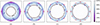 |
Figure 8. Diffuseness ψ (colormap and 90% contour) and level w normalized to origin (blue dotted 1 dB contour) of a unit circle of L={4, 6, 8, 12} equi-angle uncorrelated vertical line sources (dots) in the subfigures (a–d), compared against a circle of the relative radius |

Figure 10 (a–e) shows similar results for the rectangle/superellipse with p=10 and the continuous variance  sampled at the equi-angle directions of the corresponding t-designs, for uncorrelated, vertical line sources. Whether the
  contour actually reaches an acceptable consistency with the 90% diffuseness contour appears to strongly depend on the sampling, and in particular corners or edges can get cut-off in (a–h) with a small number of sources.
Figure 10 (e–h) analyzes equal-variance σ2=1, uncorrelated, vertical line sources whose layout solve the Thomson problem for minimum potential energy, after initialization by an equi-angular layout. There appears to be a slight difference to (a–e) by the 90% diffuseness coverage and 1 dB potential energy contours reaching corner regions a bit more closely, however occasionally not as a connected region (f, g). Sources tend to be pushed further into the corners, because with σ2=1, only the spacing between the equal-variance, discrete sources can approximate the required continuous density  .
.
4.4 Discretization study in 3D
For the sphere, there are too few equi-angle discretization schemes and spherical t-designs [36] are more useful. To define the sweet area for diffuse-field synthesis with discrete sources, the Chebyshev-type quadratures from [84–86] were chosen as t designs for discretization. Consistent with the choice above, the parameter t for the sphere is chosen to be t=2N+1.
Simulation yields results in Figure 9 that are similar to those for the circle discretized by a t=2N+1 design in Figure 8. Only now for the sphere, the number of sources needs to be much larger with L={6, 12, 24, 70} for N={1, 2, 3, 5} and t={3, 5, 7, 11}, when compared to L={4, 6, 8, 12} for the circle. This ensures that the sweet-area radius estimated in equation (27) also nicely models the ψ=90% diffuseness contour, as indicated by the orange red, dotted circle. Concerning the sound energy density, the 1 dB contour stays outside this sweet area until Figure 9 (c) with a discretization by 24 sources. The slightly non-constant sound pressure level measured by ρ c2 w appears to be negligible in practical implementations using N<4 or t-designs with t<9.
 |
Figure 9. Diffuseness ψ (colormap and 90% contour) and level w normalized to origin (blue dotted 1 dB contour) of a unit sphere of L={6, 12, 24, 70} point sources (dots) from spherical {3, 5, 7, 11} designs (Gräf, Chebyshev-type [84]) in the subfigures (a–d), compared against a relative radius |

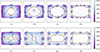 |
Figure 10. Diffuseness ψ (colormap and 90% contour) and level w normalized to origin (blue dotted 1 dB contour) of a 3:2 p=10 superellipse/rectangle of L={4, 6, 8, 12} vertical line sources (dots) using/initialized by equi-angular circular {3, 5, 7, 11} designs, with t-designs and |


Figure 11 (a–e) shows similar results for the cuboid/superellipsoid with p=10 and the continuous variance  sampled at the directions of the corresponding t-designs. Whether whether the
  contour actually reaches an acceptable consistency with the 90% diffuseness contour depends on the sampling, and in particular corners or edges can get cut off in (a–h) for the layouts with only a few points.
 |
Figure 11. Diffuseness ψ (colormap and 90% contour) and level w normalized to origin (blue dotted 1 dB contour) of a 6:4:3 p=10 superellipsoid/cuboid of L={6, 12, 24, 70} point sources (dots) using/initialized by spherical {3, 5, 7, 11} designs (Gräf, Chebyshev-type [84]), with t-designs and |


Figure 11 (e–h) shows the equal-variance σ2=1 solutions for the Thomson problem that was initialized by spherical t-design nodes. Here in 3D, these solutions appear to have clearer benefits, since their 90% diffuseness contours and their 1 dB potential energy contours reach more effectively into edge and corner regions. Sources will tend to be pushed further into these regions of the manifold that exhibit a larger radius. As in 2D, we also expect in 3D that the variation of spacing between the equal-variance σ2=1 sources has to model the continuous density  . The difference between this unit-variance solution and sampling the continuous density at given directions is most likely a more flexible customization of the source configuration to the manifold.
5 Conclusion
Building on our previous work on ideal theoretical conditions for synthesizing diffuse sound fields [34]–e.g., continuous spherical layers of uncorrelated sources–this paper explored the use of more realistic, rectangular, and discrete source layers.
We focused on achieving a high diffuseness metric ψ across an extended area. The metric ranges from 0% for the directional field of a single source to 100% for a locally diffuse sound field. To clarify its perceptual significance, we conducted a simple simulation to evaluate how it governs relevant auditory metrics. The results suggest that maintaining both low IC and low ILD near their lowest JND requires a diffuseness threshold of ψ≥90%, above which the synthesis is likely to be perceived as ideally enveloping and diffuse. Below this threshold, certain head orientations may cause ILDs to become perceptible.
While earlier work on continuous source layers with ideal geometries employed equal variance σ2=1 to synthesize a full 100% diffuseness throughout the entire volume, this study demonstrated how the same goal can be pursued for non-circular/non-spherical source layers of ideal sources. The intensity of each individual source must decay according to  , where D=2, 3 is the number of spatial dimensions. In general, these sources must also be driven by a suitable non-uniform variance σ2. As a practical parametric shape, we focused on the superellipsoid centered at the origin, whose shape-controlling parameter p can be adjusted from an ellipsoid p=2 to a rectangular cuboid as p→∞.
For 2D and 3D continuous superellipsoid layers of uncorrelated sources arranged with uniform directional density, we propose an approximate solution for the source variance:  . Here, r0 measures the distance of each source to the origin and ra the relative radius change between ellipsoid and superellipsoid.
For the ellipsoid (p=2), both in 2D and 3D, the proposed variance reduces to  as ra=1. The factor
  provides stronger activation of sources at a larger distance from the origin. This solution was proven to achieve zero intensity and, therefore, perfect diffuseness (ψ=100%) inside the ellipsoid. It was shown to be equivalent to the exact equilibrium surface-charge distribution in the analogous elliptic conductor problem in electrostatics, where the field inside is necessarily zero.
For the superellipsoid (p=10), which corresponds to a rounded rectangle/cuboid in 2D and 3D, the proposed variance  stays an approximate solution but reaches a high diffuseness of ψ>90% nearly everywhere inside the superellipsoid. The additional term
  emphasizes sources in corners and edges.
We could moreover show that providing isotropy to a central observer requires source activation by the variance  . It should be stressed that this is incompatible with the proposed variance
  for large-area synthesis of diffuseness. In particular, large-area diffuseness emphasizes anisotropy towards sources at larger radii, in edges, and corners, when compared to
  .
.
For discrete source layouts, we could define a relative radial limit  of the synthesis area achieving ψ≥90% diffuseness when using circular/spherical layouts arranged in tight spherical t=2N+1 designs.
We could show that this radial limit still serves as a rough estimate of the ψ≥90% area for ellipse/ellipsoid and rectangle/cuboid constellations, with the proposed source variance  sampled at the directions of a tight spherical t=2N+1 design.
Solving the Thomson problem was proposed as an alternative to find discrete superellipsoid source layouts driven by uniform variances σ2=1. This scenario appeared to largely adhere to the same radial limit when using a similar number of sources.
We were unable to find any other than a numerical evidence that the proposed density  is a reasonable approximation for our application. Future work could consider numerical simulations to define the limits of the approximation, and whether it could serve as supremum/infimum baseline solution for solvers in electrostatics/elasticity, in addition to more elaborated baselines, e.g. [76].
It has been found by comparison with a less robust mode-matching solution proposed in a preprint [78], for D=2 using circular, and for D=3 using spherical harmonics.
Funding
We gratefully received funding from the Austrian Science Fund (FWF): P 35254-N (Envelopment in Immersive Sound Reinforcement, EnImSo). We thank the editor and anonymous reviewers for their appreciation of the topic and guidance through substantial revisions.
Conflicts of interest
The authors declare no conflict of interest.
Data availability statement
The research data associated with this article is available in the IEM Git repository, under the reference [87].
References
- F. Jacobsen: A note on instantaneous and time-averaged active and reactive sound intensity. Journal of Sound and Vibration 147 (1991) 489–496. https://doi.org/10.1016/0022-460X(91)90496-7 [CrossRef] [Google Scholar]
- H. Kuttruff: Room acoustics, 6th edn. CRC Press, Boca Raton, 2017. https://doi.org/10.1201/9781315372150 [Google Scholar]
- J.-D. Polack: Playing billiards in the concert hall: the mathematical foundations of geometrical room acoustics. Applied Acoustics 38 (1993) 235–244. https://doi.org/10.1016/0003-682X(93)90054-A [CrossRef] [Google Scholar]
- R. Badeau: Statistical wave field theory. Journal of the Acoustical Society of America 156 (2024) 573–599. https://doi.org/10.1121/10.0027914 [CrossRef] [PubMed] [Google Scholar]
- M. Nolan, E. Fernandez-Grande, J. Brunskog, C.-H. Jeong: A wavenumber approach to quantifying the isotropy of the sound field in reverberant spaces. Journal of the Acoustical Society of America 143 (2018) 2514–2526. https://doi.org/10.1121/1.5032194 [CrossRef] [PubMed] [Google Scholar]
- M. Berzborn, M. Vorländer: Directional sound field decay analysis in performance spaces. Building Acoustics 28 (2021) 249–263. https://doi.org/10.1177/1351010X20984622 [CrossRef] [Google Scholar]
- G. Götz, S. J. Schlecht, V. Pulkki: Common-slope modeling of late reverberation. IEEE/ACM Transactions on Audio, Speech, and Language Processing 31 (2023) 3945–3957. https://doi.org/10.1109/TASLP.2023.3317572 [CrossRef] [Google Scholar]
- B. Alary, A. Politis, S. J. Schlecht, V. Välimäki: Directional feedback delay network. Journal of the Audio Engineering Society 67 (2019) 752–762. Available: https://doi.org/10.17743/jaes.2019.0026 [CrossRef] [Google Scholar]
- S. Bilbao, B. Alary: Directional reverberation time and the image source method for rectangular parallelepipedal rooms. Journal of the Acoustical Society of America 155 (2024) 1343–1352. https://doi.org/10.1121/10.0024975 [CrossRef] [PubMed] [Google Scholar]
- C.V. Hoorickx, E.P. Reynders: Numerical realization of diffuse sound pressure fields using prolate spheroidal wave functions. Journal of the Acoustical Society of America 151 (2022) 1710–1721. https://doi.org/10.1121/10.0009764 [CrossRef] [PubMed] [Google Scholar]
- O. Robin, A. Berry, O. Doutres, N. Atalla: Measurement of the absorption coefficient of sound absorbing materials under a synthesized diffuse acoustic field. Journal of the Acoustical Society of America 136 (2014) EL13–EL19. https://doi.org/10.1121/1.4881321 [CrossRef] [PubMed] [Google Scholar]
- S. Dupont, M. Sanalatii, M. Melon, O. Robin, A. Berry, J.-C. Le Roux: Measurement of the diffuse field sound absorption using a sound field synthesis method. Acta Acustica 7 (2023) 26. https://doi.org/10.1051/aacus/2023021 [CrossRef] [EDP Sciences] [Google Scholar]
- E. Habets, S. Gannot: Generating sensor signals in isotropic noise fields. Journal of the Acoustical Society of America 122 (2007) 3464–3470. https://doi.org/10.1121/1.2799929 [CrossRef] [PubMed] [Google Scholar]
- M. Kustner: Spatial correlation and coherence in reverberant acoustic fields: extension to microphones with arbitrary first-order directivity. Journal of the Acoustical Society of America 123 (2008) 152–164. https://doi.org/10.1121/1.2812592 [Google Scholar]
- N. Akbar, G. Dickins, M.R.P. Thomas, P. Samarasinghe, T. Abhayapala: A novel method for obtaining diffuse field measurements for microphone calibration, in: IEEE ICASSP, Barcelona, Spain, 4–8 May, IEEE, 2020. https://doi.org/10.1109/ICASSP40776.2020.9054728 [Google Scholar]
- G. Theile: Comparison of two dummy head systems with due regard to different fields of application, in DAGA, Darmstadt, 84a0223.pdf, 1984. Available at https://pub.dega-akustik.de/DAGA_1982-1990.zip [Google Scholar]
- T. McKenzie, D.T. Murphy, G. Kearney: Diffuse-field equalisation of binaural ambisonic rendering. Applied Science 8 (2018) 1956. https://doi.org/10.3390/app8101956 [CrossRef] [Google Scholar]
- C. Armstrong, L. Thresh, D. Murphy, G. Kearney: A perceptual evaluation of individual and non-individual HRTFs: a case study of the SADIE II database. Applied Science 8 (2018) 2029. https://doi.org/10.3390/app8112029 [CrossRef] [Google Scholar]
- D.J. Moreau, J. Ghan, B. Cazzolato, A. Zander: Active noise control in a pure tone diffuse sound field using virtual sensing. Journal of the Acoustical Society of America 125 (2009) 3742–3755. https://doi.org/10.1121/1.3123404 [CrossRef] [PubMed] [Google Scholar]
- F. Holzmüller, A. Sontacchi: Frequency limitation for optimized perception of local active noise control, in DAGA, Hamburg, 6–9, March. 2023. Available at https://pub.dega-akustik.de/DAGA_2023/data/articles/000531.pdf [Google Scholar]
- S.J. Elliott, P. Joseph, A. Bullmore, P.A. Nelson: Active cancellation at a point in a pure tone diffuse sound field. Journal of Sound and Vibration 120 (1988) 183–189. https://doi.org/10.1006/jsvi.1996.0742 [CrossRef] [Google Scholar]
- K. Hiyama, S. Komiyama, K. Hamasaki: The minimum number of loudspeakers and its arrangement for reproducing the spatial impression of diffuse sound field, in 113th AES Conv, Los Angeles, USA, 5–8 October, 2002. Available at http://www.aes.org/e-lib/browse.cfm?elib=11272 [Google Scholar]
- A. Walther, C. Faller: Assessing diffuse sound field reproduction capabilities of multichannel playback systems, in 130th AES Convention, London, UK, 13–16, May 2011. Available at http://www.aes.org/e-lib/browse.cfm?elib=15895 [Google Scholar]
- M.P. Cousins, F.M. Fazi, S. Bleeck, F. Melchior: Subjective diffuseness in layer-based loudspeaker systems with height, in 139th AES Convention, New York, USA, October 29–November 1, 2015. Available at http://www.aes.org/e-lib/browse.cfm?elib=17983 [Google Scholar]
- S. Riedel, F. Zotter: Surrounding line sources optimally reproduce diffuse envelopment at off-center listening positions. Journal of the Acoustical Society of America 2 (2022) 094404. https://doi.org/10.1121/10.0014 168 [Google Scholar]
- S. Riedel, M. Frank, F. Zotter: The effect of temporal and directional density on listener envelopment. Journal of the Audio Engineering Society 71 (2023) 455–467. Available: https://doi.org/10.17743/jaes.2022.0088 [CrossRef] [Google Scholar]
- M. Blochberger, F. Zotter, M. Frank: Sweet area size for the envelopment of a recursive and a non-recursive diffuseness rendering approach, in 5th International Conference on Spatial Audio, 26–28 September, Ilmenau, Germany, Verband Deutscher Tonmeister e.V., 2019, pp. 151–157. https://doi.org/10.22032/dbt.39969 [Google Scholar]
- P. Heidegger, B. Brands, L. Langgartner, M. Frank: Sweet area using ambisonics with simulated line arrays, in DAGA, Vienna, Austria, 15–18 August, 2021. Available at https://pub.dega-akustik.de/DAGA_2021/data/articles/000374.pdf [Google Scholar]
- S. Riedel, L. Gölles, M. Frank, F. Zotter: Modeling the listening area of envelopment. in DAGA, Hamburg, Germany, 6–9 March, 2023. Available at https://pub.dega-akustik.de/DAGA_2023/data/articles/000289.pdf [Google Scholar]
- S. Riedel, M. Frank, F. Zotter, R. Sazdov: A study on loudspeaker SPL decays for envelopment and engulfment across an extended audience, in AES 2024 International Acoustics & Sound Reinforcement Conference, Le Mans, France, 23–26 January, 2024. Available at http://www.aes.org/e-lib/browse.cfm?elib=22368 [Google Scholar]
- T. Tanaka, M. Otani: An isotropic sound field model composed of a finite number of plane waves. Acoustical Science and Technology 44 (2023) 4. https://doi.org/10.1250/ast.44.317 [CrossRef] [Google Scholar]
- T. Tanaka, M. Otani: Spatially characterized pseudo-perfect diffuseness via finite-degree spherical harmonic diffuseness. JASA Express Letters 4 (2024) 071601. https://doi.org/10.1121/10.0026466 [CrossRef] [PubMed] [Google Scholar]
- T. Tanaka, M. Otani: Directionally characterized pseudo-perfect diffuseness: a detailed comparison of its theoretical formulations. Acoustical Science and Technology 45 (2024) 260–269. https://doi.org/10.1250/ ast.e24.16 [CrossRef] [Google Scholar]
- F. Zotter, S. Riedel, L. Gölles, M. Frank: Diffuse sound field synthesis: idela source layers. Acta Acustica 34 (2024) 16. https://doi.org/10.1051/aacus/2024023 [Google Scholar]
- I. Newton: The mathematical principles of natural philosophy, B. Motte, 1729, tranlation by Andrew Motte. Available at https://en.wikisource.org/wiki/The_ Mathematical_Principles_of_Natural_Philosophy_(1729) [Google Scholar]
- P. Delsarte, J. Goethals, J. Seidel: Spherical codes and designs, in Geometry and combinatorics, D.G. Corneil, R. Mathon (Eds.), Academic Press, 1991, pp. 68–93. https://doi.org/10.1016/B978-0-12-189420-7.50013-X [CrossRef] [Google Scholar]
- F. Jacobsen, T. Roisin: The coherence of reverberant sound fields. Journal of the Acoustical Society of America 108 (2000) 204–210. https://doi.org/10.1121/1.429457 [CrossRef] [PubMed] [Google Scholar]
- R. Nicol: Restitution sonore spatialisée sur une zone étendue: application á la téléprésence. PhD dissertation, Université du Maine, 1999. Available at https://theses.hal.science/tel-01067541/document [Google Scholar]
- J. Daniel: Représentation de champs acoustiques, application á la transmission et á la reproduction de scénes sonores complexes dans un contexte multimédia. PhD dissertation, Université de Paris 6, 2001. Available at http://gyronymo.free.fr/audio3D/downloads/These-original-version.zip [Google Scholar]
- D. Ward, T. Abhayapala: Reproduction of a plane-wave sound field using an array of loudspeakers. IEEE Transactions on Speech and Audio Processing 9 (2001) 697–707. https://doi.org/10.1109/89.943347 [CrossRef] [Google Scholar]
- R.A. Kennedy, P. Sadeghi, T.D. Abhayapala, H.M. Jones: Intrinsic limits of dimensionality and richness in random multipath fields. IEEE Transactions on Signal Processing 55 (2007) 2542–2556, 2007. https://doi.org/10.1109/TSP.2007.893738 [CrossRef] [Google Scholar]
- M.A. Poletti: Three-dimensional surround sound systems based on spherical harmonics. Journal of the Audio Engineering Society 53 (2005) 1004–1025. http://www.aes.org/e-lib/browse.cfm?elib=13396 [Google Scholar]
- J. Ahrens: Analytic methods of sound field synthesis. Springer, 2012. https://doi.org/10.1007/978-3-642-25743-8 [CrossRef] [Google Scholar]
- P. Grandjean, A. Berry, P.-A. Gauthier: Sound field reproduction by combination of circular and spherical higher-order ambisonics: part I – a new 2.5-D driving function for circular arrays. Journal of the Audio Engineering Society 69 (2021) 152–165. Available at http://www.aes.org/e-lib/browse.cfm?elib=21024 [CrossRef] [Google Scholar]
- P. Stitt, S. Bertet, M. van Walstijn: Off-centre localisation performance of ambisonics and hoa for large and small loudspeaker array radii. Acta Acustica united with Acustica 100 (2014) 937–944. https://doi.org/10.3813/AAA.918773 [CrossRef] [Google Scholar]
- M. Frank, F. Zotter: Exploring the perceptual sweet area in ambisonics, in 142nd AES Convention, Berlin, Germany, 20–23 May, 2017. http://www.aes.org/e-lib/browse.cfm?elib=18604 [Google Scholar]
- F. Zotter, M. Frank: Ambisonics. SpringerOpen, Cham, 2019. https://doi.org/10.1007/978-3-030-17207-7 [CrossRef] [Google Scholar]
- K. Merimaa, V. Pulkki: Spatial impulse response rendering I: analysis and synthesis. Journal of the Audio Engineering Society 53, (2005) 1115–1127. http://www.aes.org/e-lib/browse.cfm?elib=13401 [Google Scholar]
- J. Merimaa: Energetic sound field analysis of stereo and multichannel loudspeaker reproduction, in 123rd AES Convention, 5–8 October, New York, NY, 2007. http://www.aes.org/e-lib/browse.cfm?elib=14315 [Google Scholar]
- T.L. Curtright, Z. Cao, S. Huang, J.S. Sarmiento, S. Subedi, D.A. Tarrence, T.R. Thapaliya: Charge densities for conducting ellipsoids. European Journal of Physics 41 (2020) 035204. https://doi.org/10.1088/1361-6404/ab806a [CrossRef] [Google Scholar]
- I.V. Lindell: Charge density on a conducting ellipsoid and an elliptic disk. American Journal of Physics 65 (1997) 1113–1114. https://doi.org/10.1119/1.18731 [CrossRef] [Google Scholar]
- W. Thomson: Reprint of Papers on Electricity and Magnetism, 2nd edn. MacMillan, London, 1884. Available at https://openlibrary.org/books/OL24349305M [Google Scholar]
- Y.V. Samukhina, N.E. Rusakova, P.A. Polyakov: Dependence of surface charge density on curvature of surface of conductive body with complicated shape. Journal of Electrostatics 125 (2023) 103844. Available at https://www.sciencedirect.com/science/article/pii/S0304388623000530 [CrossRef] [Google Scholar]
- K. Bhattacharya: On the dependence of charge density on surface curvature of an isolated conductor. Physica Scripta 91 (2016) 035501. https://doi.org/10.1088/0031-8949/91/3/035501 [CrossRef] [Google Scholar]
- A.D. Alawneh, R.P. Kanwal: Singularity methods in mathematical physics. SIAM Review 19 (1977) 437–471. http://www.jstor.org/stable/2029614 [CrossRef] [Google Scholar]
- W. Hwang: A regularized boundary integral method in potential theory. Computer Methods in Applied Mechanics and Engineering 259 (2013) 123–129. https://doi.org/10.1016/j.cma.2013.02.005 [CrossRef] [Google Scholar]
- D. Caratelli, J. Gielis, I. Tavkhelidze, P.E. Ricci: The dirichlet problem for the laplace equation in supershaped annuli. Boundary Value Problems 113 (2013) 1. https://doi.org/10.1186/1687-2770-2013-113 [Google Scholar]
- B. Makhdum, A. Nadim: Dynamics and equilibria of n point charges on a 2D ellipse or a 3D ellipsoid. Applied Mathematics 14 (2023) 4. https://doi.org/10.4236/am.2023.144015 [Google Scholar]
- D. P. Hardin, E. B. Saff: Discretizing manifolds via minimum energy points. Notices of the AMS 51 (2004) 1186–1194. https://www.ams.org/journals/notices/200410/fea-saff.pdf [Google Scholar]
- J. Fliege, U. Maier: The distribution of points on the sphere and corresponding cubature formulae. IMA Journal of Numerical Analysis 19 (1999) 317–334. https://doi.org/10.1093/imanum/19.2.317 [CrossRef] [Google Scholar]
- J. Korevaar, J. Meyers: Spherical faraday cage for the case of equal point charges and chebyshev-type quadrature on the sphere. Integral Transforms and Special Functions 1 (1993) 105–117. https://doi.org/10.1080/10652469308819013 [CrossRef] [Google Scholar]
- F. Fahy: Foundations of engineering acoustics. Elsevier Academic Press, San Diego, 2001. https://doi.org/10.1016/B978-0-12-247665-5.50025-4 [Google Scholar]
- V. Pulkki: Spatial sound reproduction with directional audio coding. Journal of the Audio Engineering Society 55 (2007) 503–516. http://www.aes.org/e-lib/browse.cfm?elib=14170 [Google Scholar]
- J.J. Zwislocki, H.N. Jordan: On the relations of intensity JNDs to loudness and neural noise. Journal of the Acoustical Society of America 79 (1986) 772–780. https://doi.org/10.1121/1.393467 [CrossRef] [PubMed] [Google Scholar]
- T. Slade, A. Gascon, G. Comeau, D. Russell: Just noticeable differences in sound intensity of piano tones in non-musicians and experienced pianists. Psychology of Music 51 (2023) 924–937. https://doi.org/10.1177/03057356221126203 [CrossRef] [Google Scholar]
- A. Avni, B. Rafaely: Interaural cross correlation and spatial correlation in a sound field represented by spherical harmonics. in: Proceedings of 1st Ambisonics Symposium, Graz, Austria, 25–27 July, 2009. Available at https://iaem.at/ambisonics/symposium2009/proceedings/ambisym09-avnirafaely-iaccspatcorrsh.pdf [Google Scholar]
- J. Merimaa, V. Pulkki: Spatial impulse response rendering, in Proceedings of the DAFx, Naples, Italy, 5–8 October, 2004 [Google Scholar]
- A. Walther, C. Faller: Interaural correlation discrimination from diffuse field reference correlations. Journal of the Acoustical Society of America 133 (2013) 1496–1502. https://doi.org/10.1121/1.4790473 [CrossRef] [PubMed] [Google Scholar]
- W.M. Hartmann, Z.A. Constan: Interaural level differences and the level-meter model. Journal of the Acoustical Society of America 112 (2002) 1037–1045. https://doi.org/10.1121/1.1500759 [CrossRef] [PubMed] [Google Scholar]
- I. Pollack, W. Trittipoe: Binaural listening and interaural noise cross correlation. Journal of the Acoustical Society of America 31 (1959) 1250–1252. https://doi.org/10.1121/1.1907852 [CrossRef] [Google Scholar]
- B. Bernschütz: A spherical far field HRIR/HRTF compilation of the neumann KU 100, in 39th DAGA (AIA-DAGA), Merano, Italy, 18–21 March, 2013, pp. 592–595. https://doi.org/10.5281/zenodo.3928297 [Google Scholar]
- A.H. Barr: Superquadrics and angle-preserving transformations. IEEE Computer Graphics and Applications 1 (1981) 11–23. https://doi.org/10.1109/MCG.1981.1673799 [CrossRef] [Google Scholar]
- J. Gielis: Superellipses to superformula: the impact of gielis transformations. Research Outreach 125 (2021). https://doi.org/10.13140/RG.2.2.26896.64005/2 [Google Scholar]
- J.A. Thorpe: Elementary topics in differential geometry. Springer, New York, 1979. https://doi.org/10.1007/978-1-4612-6153-7 [CrossRef] [Google Scholar]
- W. Kühnel: Differentialgeometrie: Kurven-Flächen-Mannigfaltigkeiten, 6th edn. Springer Spektrum, Wiesbaden, 2013. https://doi.org/10.1007/978-3-658- 00615-0 [CrossRef] [Google Scholar]
- D. Caratelli, P. Ricci, J. Gielis: The robin problem for the laplace equation in a three-dimensional starlike domain. Applied Mathematics and Computation 218 (2011) 713–719, 2011, special Issue in Honour of Hari M. Srivastava on his 70th Birth Anniversary. https://www.sciencedirect.com/science/article/pii/S0096300311005261 [Google Scholar]
- D. Caratelli, P. Natalini, P.E. Ricci: Spherical harmonic solution of the robin problem for the laplace equation in supershaped shells, in Modeling in Mathematics, J. Gielis, P. E. Ricci, and I. Tavkhelidze (Eds.), Atlantis Press, Paris, 2017, pp. 17–30. https://doi.org/10.2991/978-94-6239-261-8_2 [Google Scholar]
- F. Zotter, S. Riedel, L. Gölles, M. Frank: Diffuse sound field synthesis, 2024. Available at https://arxiv.org/abs/2402.11330 [Google Scholar]
-
L. Gegenbauer: Über die Functionen
 . Sitzungsberichte der Kaiserlichen Akademie der Wissenschaften. Mathematisch-Naturwissenschaftliche Classe 57 (1877) 8. Available at https://viewer.acdh.oeaw.ac.at/viewer/image/MN_2Abt_75_1877/904/LOG_0074/
[Google Scholar]
. Sitzungsberichte der Kaiserlichen Akademie der Wissenschaften. Mathematisch-Naturwissenschaftliche Classe 57 (1877) 8. Available at https://viewer.acdh.oeaw.ac.at/viewer/image/MN_2Abt_75_1877/904/LOG_0074/
[Google Scholar]
- F.W.J. Olver, A.B. Olde Daalhuis, D.W. Lozier, B.I. Schneider, R.F. Boisvert, C.W. Clark, B.R. Miller, B.V. Saunders, H.S. Cohl, M.A. McClain, Eds. NIST Digital Library of Mathematical Functions Release 1.1.9 of 2023-03-15. Available at https://dlmf.nist.gov/ [Google Scholar]
- J.J. Thomson: Xxiv. on the structure of the atom: an investigation of the stability and periods of oscillation of a number of corpuscles arranged at equal intervals around the circumference of a circle; with application of the results to the theory of atomic structure. Philosophical Magazine Series 39 (1904) 7. http://doi.org/10.1080/14786440409463107 [Google Scholar]
- L. Föppl: Stabile anordnungen von elektronen im atom. Journal für die Reine und die Angewandte Mathematik (1912). Available: https://www.digizeitschriften.de/id/243919689_0141 [Google Scholar]
- H. Harbrecht, W.L. Wendland, N. Zorii: Rapid solution of minimal riesz energy problems. Numerical Methods for Partial Differential Equations 32 (2016) 1535–1552. https://doi.org/10.1002/num.22060 [CrossRef] [Google Scholar]
- M. Gräf: Quadrature rules on manifolds. Available at https://www-user.tu-chemnitz.de/ potts/workgroup/graef/quadrature/ (accessed 2023/04/23) [Google Scholar]
- M. Gräf: Efficient algorithms for the computation of optimal quadrature points on riemannian manifolds. PhD dissertation, Chemnitz University of Technology, 2013. Available at https://www-user.tu-chemnitz.de/ potts/workgroup/graef/quadrature/papers/Gr13Diss.pdf [Google Scholar]
- M. Gräf and D. Potts: On the computation of spherical designs by a new optimization approach based on fast spherical fourier transforms. Numerische Mathematik 119 (2011) 699–724. https://doi.org/10.1007/s00211-011-0399-7 [CrossRef] [Google Scholar]
- F. Zotter, S. Riedel, L. Gölles, M. Frank: Source code for diffuse sound field synthesis, 2023. Available at https://git.iem.at/enimso/2023-diffuse-soundfield-synthesis-acta-jupyter-code [Google Scholar]
Cite this article as: F. Zotter, S. Riedel, L. Gölles, M. Frank. 2025. Diffuse sound field synthesis: Towards practical source layouts. Acta Acustica 9, 33. https://doi.org/10.1051/aacus/2025018.
All Tables
Green's function of the potential equation in D=1, 2, 3 space dimensions and their derivative.
All Figures
|
Figure 1. Rounded cuboid S enclosing V, locations: orig. 0, src. xs, rec. x, directions: u0, u, ux, n, distances: r0, x, xmax, r, elements/angles: dS, dΩ0, dΩ, ϕ0, ϕ. |
| In the text | |
|
Figure 2. Interaural coherence (IC) and interaural level difference (ILD) evaluated for sound fields of varied diffuseness 0≤ψ≤1. The evaluation uses a variably-weighted mix of a 2D/3D diffuse sound field with a single plane wave from a horizontal, frontal azimuth angle. Gray areas indicate one just-noticeable difference (JND) from a diffuse-field reference with IC =0, ILD =0. |
| In the text | |
|
Figure 3. Diffuseness ψ (colormap, solid contour: 90%) and level w normalized to origin (dotted 1 dB contour) for 2D, 3:2 ellipse of 100 equi-angle uncorrelated vertical line sources (a–d) or 6:4:3 ellipsoid of 2500 maximum determinant nodes with uncorrelated point sources (e–h): (a, e) with unity variance σ2=1, (b, f) isotropy-enforcing variance |
| In the text | |
|
Figure 4. Directional intensity dI/dΩ0=σ2/r0 in 2D, normalized at 0°, observed at x=0 for different azimuth angles to between 0° and 90° (quadrants are symmetric) for 2:3 2D horizontal ellipse/rectangle of uncorrelated vertical line sources (superellipse p=10) with different variances σ2; isotropy requires σ2=r0. |
| In the text | |
|
Figure 5. Diffuseness ψ (colormap, solid contour: 90%) and level w normalized to origin (dotted 1 dB contour), for the rectangle of the ratio 3:2 (2D), and for the cuboid of the ratio 6:4:3 (3D), both with p=10, using 100 equi-angular nodes as uncorrelated line vertical sources (2D) or 2500 maximum determinant nodes as uncorrelated point sources (3D), respectively: (e, i) with unity gain σ2=1,(f, j) isotropy-enforcing gain |
| In the text | |
|
Figure 6. Directional intensity |
| In the text | |
|
Figure 7. Cross-section: 6:4:3 rectangular cuboid, superellipse p=10: cut1, 2 are rotated by 0°, 36.9° wrt. x. |
| In the text | |
|
Figure 8. Diffuseness ψ (colormap and 90% contour) and level w normalized to origin (blue dotted 1 dB contour) of a unit circle of L={4, 6, 8, 12} equi-angle uncorrelated vertical line sources (dots) in the subfigures (a–d), compared against a circle of the relative radius |
| In the text | |
|
Figure 9. Diffuseness ψ (colormap and 90% contour) and level w normalized to origin (blue dotted 1 dB contour) of a unit sphere of L={6, 12, 24, 70} point sources (dots) from spherical {3, 5, 7, 11} designs (Gräf, Chebyshev-type [84]) in the subfigures (a–d), compared against a relative radius |
| In the text | |
|
Figure 10. Diffuseness ψ (colormap and 90% contour) and level w normalized to origin (blue dotted 1 dB contour) of a 3:2 p=10 superellipse/rectangle of L={4, 6, 8, 12} vertical line sources (dots) using/initialized by equi-angular circular {3, 5, 7, 11} designs, with t-designs and |
| In the text | |
|
Figure 11. Diffuseness ψ (colormap and 90% contour) and level w normalized to origin (blue dotted 1 dB contour) of a 6:4:3 p=10 superellipsoid/cuboid of L={6, 12, 24, 70} point sources (dots) using/initialized by spherical {3, 5, 7, 11} designs (Gräf, Chebyshev-type [84]), with t-designs and |
| In the text | |
Current usage metrics show cumulative count of Article Views (full-text article views including HTML views, PDF and ePub downloads, according to the available data) and Abstracts Views on Vision4Press platform.
Data correspond to usage on the plateform after 2015. The current usage metrics is available 48-96 hours after online publication and is updated daily on week days.
Initial download of the metrics may take a while.