| Issue |
Acta Acust.
Volume 9, 2025
Topical Issue - Spatial and binaural hearing: From neural processes to applications
|
|
|---|---|---|
| Article Number | 74 | |
| Number of page(s) | 14 | |
| DOI | https://doi.org/10.1051/aacus/2025054 | |
| Published online | 27 November 2025 | |
Scientific Article
A binaural implementation of the Hearing Aid Speech Perception Index (HASPI)
1
Deptartment of Speech, Language, and Hearing Sciences, University of Colorado, Boulder, Colorado, USA
2
ENPTE, Ecole Centrale de Lyon, CNRS, LTDS, UMR5513, 69518 Vaulx-en-Velin, France
3
Department of Communication Sciences and Disorders, University of Northern Colorado, Greeley, Colorado, USA
* Corresponding author: This email address is being protected from spambots. You need JavaScript enabled to view it.
Received:
21
February
2025
Accepted:
14
October
2025
Abstract
Introduction: The Hearing Aid Speech Perception Index version 2 (HASPI v2) is an intrusive speech intelligibility metric fitted to the intelligibility of sentence stimuli presented monaurally over headphones. It compares the time-frequency envelope modulation of a degraded signal, processed through a peripheral model matched to the subject’s audiogram, to the envelope modulation of an unprocessed noise-free signal processed through a normal-hearing (NH) peripheral model. This paper presents a binaural extension of HASPI v2. Methods: The binaural modifications are increasing the indicated hearing loss and providing a model of binaural interaction. The binaural HASPI was fit to binaural sentence-level intelligibility scores for NH and hearing-impaired (HI) subjects. The experimental conditions comprised combinations of room acoustics, spatial source configuration, noise, and simulated hearing-aid processing. Results: The Pearson correlation coefficients between the binaural HASPI predictions and the observed binaural intelligibility scores were 0.982 for the NH group, 0.981 for the HI group, and 0.983 for the combined groups. The corresponding RMS errors for intelligibility scores on a 0 to 1 scale were 0.050, 0.049, and 0.049. Discussion and Conclusions: The accuracy of the binaural HASPI is similar for HI and NH subjects. The accuracy compares favorably to that of existing binaural metrics.
Key words: Speech intelligibility / Binaural hearing / Binaural intelligibility / Intelligibility prediction models / Hearing aids
© The Author(s), Published by EDP Sciences, 2025
 This is an Open Access article distributed under the terms of the Creative Commons Attribution License (https://creativecommons.org/licenses/by/4.0), which permits unrestricted use, distribution, and reproduction in any medium, provided the original work is properly cited.
1. Introduction
The Hearing Aid Speech Perception Index (HASPI) [1–3] is an intrusive intelligibility metric in which the time-frequency envelope modulation of a degraded sentence is compared to that for a noise- and distortion-free reference sentence. The current implementation is HASPI version 2 (HASPI v2) [2, 3]. HASPI v2 is designed to deal with a wide range of speech degradations such as additive noise, reverberation, nonlinear distortion, and hearing-aid (HA) processing. The basic structure of HASPI v2 is a model of the auditory periphery followed by time-frequency envelope modulation analysis and an ensemble of neural networks that transform the envelope modulation correlations between degraded and reference signals into subject sentence-level intelligibility scores. The peripheral model is not meant to be a complete representation of auditory physiology; rather, it is meant to reproduce a salient subset of physiological and perceptual behaviors that can be used by the curve-fitting back end of the system to fit the subject data. The peripheral model can be adjusted based on the subject’s audiogram, making HASPI v2 appropriate for both normal-hearing (NH) and hearing-impaired (HI) subjects. For NH subjects both the degraded and reference signals are passed through models of the normal auditory periphery, while for HI subjects the amplified degraded signal is passed through a model of the impaired periphery while the reference signal is passed through a model of the normal periphery.
HASPI v2 was fitted to intelligibility scores for sentence stimuli presented monaurally over headphones. The monaural headphone presentation is a potential limitation of the metric since it bypasses the cues used for spatial unmasking of speech [4, 5]. For binaural listening, spatial separation of the speech and noise sources provides interaural level differences (ILD) and interaural time differences (ITD) between the two ears. The ILD can lead to different signal-to-noise ratios (SNRs) at the left and right ears, an effect exploited by better-ear listening wherein intelligibility is determined by the ear having the higher SNR in each auditory frequency band. The ITD can introduce interaural phase differences that can lead to binaural unmasking of the target speech [6] and which can be modeled using the equalization-cancellation (EC) theory [7, 8] or via interaural cross-correlation [9].
The objective of this paper is to develop a binaural version of HASPI v2 by combining the HASPI v2 peripheral model and envelope modulation analysis with a model of binaural interaction. The general approach of combining a monaural intelligibility metric with a binaural model has been adopted in most binaural intelligibility models. The most common approach is to use an EC front end combined with the speech intelligibility index (SII) [10] to predict intelligibility [11–14]. The EC front end has also been modified and combined with other monaural speech intelligibility predictors including the Short-Time Objective Intelligibility metric (STOI) [15] to produce the Deterministic Binaural STOI (DBSTOI) [16] and the Modified Binaural STOI (MBSTOI) [17], and also combined with the envelope power SNR [18, 19]. Several of these models (e.g. [17–19]) combine simplified interaural processing related to an EC front end with better-ear SNR estimates, and the results presented in [20] suggest that better-ear glimpsing may also make an important contribution to binaural intelligibility.
An interaural cross-correlation front end has also been effectively combined with the speech transmission index (STI) [21] to yield binaural intelligibility predictions relevant to room acoustics [22]. Other approaches include using the HASPI peripheral model at each ear followed by a deep neural network (DNN) to estimate the binaural interaction [23, 24] or directly estimating the binaural masking level difference (BMLD) from the left and right ear signals [6, 25, 26]. Most of these papers only deal with NH subjects, although some also consider HI subjects [12, 23, 24, 27]. The general success of these combined models suggests that modifying HASPI v2 by adding a model of binaural interaction should also lead to accurate binaural intelligibility predictions.
The EC theory assumes that the auditory system adjusts the interaural amplitude and phase of the noisy speech in each frequency band to minimize the residual noise power when the left and right ear signals are delayed, weighted, and subtracted [7, 8, 13]. While several of the studies cited above indicate that the EC approach may be appropriate for noisy speech, this approach may not be valid for HA processed speech where the processing introduces nonlinear distortion that can be highly correlated with the speech signals [28]. An alternative approach to modeling binaural interaction is an auditory filterbank followed by dynamic-range compression and envelope extraction at each ear [9]; the compressed left- and right-ear envelopes are then cross-correlated to give the perceptual decision variable. This envelope cross-correlation approach is consistent with the structure of HASPI v2 and is therefore an attractive candidate to use in developing the binaural implementation.
The remainder of this paper presents the design and evaluation of the binaural HASPI. The binaural intelligibility data are presented in the next section; sentence-level intelligibility scores were obtained for NH and HI subjects for a variety of noise, acoustic, and HA processing conditions. The structure of the binaural HASPI is then described and contrasted with the monaural HASPI v2. The predictions for the binaural intelligibility data are then presented, including the adjustment to the peripheral hearing loss for modeling binaural intelligibility and comparisons between the better-ear values for the monaural HASPI v2 and the binaural HASPI and between NH and HI subjects. The paper concludes with a discussion of the model results and their accuracy and a final summary.
2. Intelligibility data
The binaural HASPI metric was fitted to a binaural intelligibility dataset scored for sentences correct [29]. An extensive description of the dataset is provided in [29], so only a summary is provided here. Data were acquired from 15 younger adult NH (mean age 22 years, age range 19–28 years) and 15 older adult HI (mean age 78 years, age range 57–84 years) subjects having symmetric bilateral mild to moderately-severe sensorineural hearing losses; audiograms averaged across the two ears are provided in Figure 1. The experiment used dummy-head head-related impulse response (HRIR) recordings and binaural headphone stimulus presentation. A total of 54 processing conditions were implemented, comprising all possible combinations of two simulated acoustic spaces, three spatial configurations of the speech and noise sources, three SNRs, and three simulated hearing-aid processing settings.
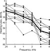 |
Figure 1. Audiograms in dB HL for the HI subjects averaged across the two ears. The individual audiograms are indicated by the dashed lines and the group average by the solid black line (from Kates et al. [29]). |
The two simulated acoustic spaces were an anechoic room and a concert hall. The simulations used recordings from a horizontal loudspeaker array located in a semi-anechoic chamber that also contained electronics associated with audio-visual signal presentation and recording. The loudspeakers were located at 10-degree increments in a full circle around the periphery of the chamber, and a virtual-image “shoebox” room simulation [30] system controlled the inputs to the loudspeakers to create the acoustic environments that included the propagation delays and power-law attenuation for each virtual image. Atmospheric sound absorption was added using the procedure of [31], which reduced the metallic artifacts that can occur in simulated reverberation. The resultant simulated concert hall had a reverberation time (RT) of 2.4 s and a direct-to-reverberant ratio (DRR) of 4.3 dB when measured for the center front speech source 1.9 m in front of the dummy head. The virtual image matrix used for the room simulation incorporated all reflections out to 2.6 s.
A sentence embedded in continuous discourse may be masked by the reverberant tail of a preceding sentence. This energetic masking was simulated by concatenating a time-reversed version of the sentence in front of the normal-time version, processing the sentence pair through the simulated reverberation, and then removing the time-reversed sentence, thus leaving the reverberant tail overlaying the beginning of the normal-time sentence. The time reversal preserves the sentence envelope statistics and long-term spectrum while minimizing intelligibility. After reverberation was applied to both the speech and the noise, the preceding sentence with its associated noise was pruned, leaving the noisy target sentence with its onset masked by the reverberant tail from the time-reversed noisy sentence. The input signals for the HA processing were recorded using commercial HA microphones located in behind-the-ear (BTE) shells mounted behind the ears of the KEMAR manikin [32], and ear-canal signals were recorded simultaneously from the manikin ears. The left and right front HA microphones provided the input signals for the simulated HA processing. Ear-canal responses were also recorded simultaneously from both ears of KEMAR. The recorded microphone signals thus included the simulated room reverberation (if present) and the KEMAR HRIR associated with each loudspeaker location.
The HA simulation combined the KEMAR microphone recordings with the HA processing, with the processing operating independently in the two ears [33]. The processing simulated a six-channel hearing aid. The inputs to the left and right hearing aids were the speech and noise stimuli convolved with the reverberation and the KEMAR HA microphone and ear canal responses. Frequency analysis was implemented using a six-channel linear-phase finite impulse response (FIR) filterbank having band center frequencies at (250, 500, 1000, 2000, 4000, and 6000) Hz. The HA processing within each frequency band used a series configuration, with noise suppression first followed by WDRC and then frequency compression.
Noise suppression for both the NH and HI subjects was implemented with an adaptive Wiener filter [34] where the gain in each frequency band depended on the ratio of the short-time speech power to the noise power averaged over the entire stimulus; more information is provided in [29, 34]. Compensation for the hearing impairment was provided by either NAL-R linear amplification [35] or NAL-NL2 wide dynamic-range compression (WDRC) [36] having a 5 ms attack time and a 50 ms release time. High frequencies for the HI subjects were shifted lower to fit into their impaired auditory bandwidths using frequency compression based on sinusoidal modeling [37]. A flat receiver frequency response was used and the system simulated earmold venting with a radius of 0.6 cm [38]; the venting was simulated by a complementary pair of 2nd order highpass and lowpass filters having cutoff frequencies of 350 Hz, with the ambient ear canal signal passed through the lowpass filter without modification and the HA output passed through the highpass filter.
Three HA processing settings were used for the NH subjects: (1) a flat 0 dB gain, (2) noise suppression with a maximum attenuation of 6 dB, and (3) noise suppression with a maximum attenuation of 12 dB. For the HI subjects, the three processing settings were (1) linear NAL-R amplification, (2) WDRC plus noise suppression limited to 6 dB, and (3) WDRC plus noise suppression limited to 12 dB and frequency compression matched to the audiogram. The frequency compression was applied above the specified cutoff frequency and bypassed below; the cutoff frequencies ranged from 4.7 to 2.0 kHz and the associated compression ratios ranged from 2.9 to 1.5 as the loss went from mild to severe [39].
Intelligibility was scored as the proportion completely correct IEEE sentences [40] for stimuli presented at 65 dB SPL. The sentences were spoken by 15 male and 18 female talkers [41]. The combination of talker, IEEE list, and sentence within the list was chosen at random for each processed sentence presented to each subject. The speech was mixed with two six-talker babble sources [42] at SNRs of 3, 8, and 20 dB [43] for three spatial configurations: (1) speech and both noise sources collocated at 0 deg (directly in front of the subject), (2) speech at 0 deg and noise at ±60 deg, and (3) speech at 60 deg and noise at 0 and −60 deg; a positive angle is towards the subject’s right. The SNRs were computed as the ratio of the power in the speech signal averaged across the left and right HA microphones in the selected room simulation (anechoic or concert hall) to the power in the composite noise signal averaged across the two HA microphones for the same room simulation. The experiment comprised 54 processing conditions: 2 simulated rooms × 3 SNRs × 3 spatial configurations × 3 HA settings, with 10 randomized repetitions of each condition for each subject.
For the stimulus presentation, each subject was seated in a sound isolation booth. Stimuli were presented through Sennheiser HD-25 headphones, and the subjects repeated back the sentences that they heard. Compensation for the headphone response was not provided, but the dummy head headphone response is flat within ±3 dB from approximately 40 to 4000 Hz. A short unscored training session comprising ten sentences was provided for acclimation, after which the test sentences were played out and scored; two sessions of approximately 1.5–2 h each were needed for the complete experiment.
3. Intelligibility metric
The binaural HASPI is an extension of HASPI v2 [3]. It uses the same basic model of the auditory periphery [44] for the left and right ears, but the peripheral model parameters are adjusted for binaural hearing and are followed by a model of binaural interaction; explanations of these modifications are provided in Section 3.2. The output of the binaural interaction model is in turn evaluated using an envelope modulation analysis that is the same as used for HASPI v2. An ensemble of neural networks is then used to transform the time-frequency envelope modulation measurements to the binaural subject intelligibility scores, with the neural networks designed using the same procedure as for HASPI v2. Each of these processing steps is described below.
3.1. Peripheral model
The overall block diagram for the peripheral model is shown in Figure 2. The reference signal is the average of the left and right ear-canal signals for the test sentence reproduced in an anechoic environment; the averaging smooths out the slight differences between the KEMAR left and right ears. The left and right ear degraded signals can include compensation for hearing loss (for HI subjects) as well as the room, noise, and processing effects. The signal sampling rates are all converted to 24 kHz, followed by broadband temporal alignment of the left and right ear signals to the reference signal. A second temporal alignment stage is later provided within each frequency band. For both NH and HI subjects the reference signal is passed through a model of the NH periphery. The left and right ear degraded signals for the NH subjects are also passed through a model of the NH periphery, while the degraded signals for the HI subjects are passed through a model of the HI periphery.
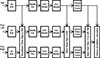 |
Figure 2. Binaural HASPI block diagram showing the comparison of the left and right ear signals with the reference signal. |
A more detailed block diagram for the peripheral model used for both NH and HI ears is presented in Figure 3. After sampling-rate conversion, the signal is passed through a middle ear filter [45], followed by an auditory frequency analysis and a separate control filterbank. Both filterbanks use a 4th-order gammatone filterbank [46, 47]; 32 filters span the frequency range from 80 to 8000 Hz. The auditory filter bandwidths are determined by the RMS level measured over the duration of the sentence when passed through the control filterbank and are held constant over the sentence duration. The control filter bandwidths for both NH and HI subjects are set to the widest values used in the model and correspond to the auditory filters adjusted for the greatest hearing loss and/or highest signal intensity. The maximum relative bandwidth of the control filters increases with increasing frequency and is 4 times normal at 8 kHz. The auditory filter bandwidths for HI subjects [48] are wider than those for NH subjects [49], and the filter bandwidths for both NH and HI subjects within each band increase with increasing signal intensity above 50 dB SPL [44, 50, 51].
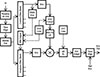 |
Figure 3. Binaural HASPI block diagram of the auditory model used to extract the signal envelopes in each frequency band. |
The control filterbank outputs also control the dynamic-range compression mediated by the outer hair cells (OHC) [52]. The envelopes of the control filter output signals in each band are passed through an 800 Hz lowpass filter [53] to provide a small time delay. The amplitudes of the filtered envelopes control the gains applied to the auditory filter outputs in each band. Linear amplification is applied to inputs below 30 or above 100 dB SPL while amplitude compression is applied to signals lying between 30 and 100 dB SPL. The compression ratio for NH listeners ranges from 1.25:1 at 80 Hz to 3.5:1 at 8 kHz. The OHC damage associated with hearing loss shifts the auditory threshold upwards and reduces the compression ratio. For the maximum allowed hearing loss of 100 dB, the system reverts to linear amplification with the output for an input at 100 dB SPL matched to the NH output for the same signal intensity.
Following compression, the envelope in each auditory band is converted to dB re auditory threshold with sound levels below threshold set to a lower limit of 0 dB SL plus a 0.1 dB dither. Inner hair cell (IHC) damage is modeled as additional envelope attenuation, and IHC adaptation is applied to the envelope dB output using a rapid time constant of 2 ms and a short-term time constant of 60 ms [54]. A final in-band time alignment is applied to align the left and right ear envelope signals with the reference signals, followed by compensation for the delays associated with the auditory filters [55].
3.2. Binaural modifications
In addition to adjusting the peripheral model parameters for separate audiograms at the two ears, the left and right ear models are further adjusted for binaural hearing. The auditory filters for binaural hearing, when measured using a notched-noise paradigm, are wider than the filters measured monaurally in both NH and HI subjects [56, 57]. An auditory model incorporating contralateral inhibition between the left- and right-ear frequency bands has been proposed to account for this apparent difference [58]. However, broader auditory filters can also be induced in the HASPI v2 peripheral model by adjusting the audiogram passed to the model. This simpler approach is based on multiplying the measured hearing loss by an audiogram scale factor greater than 1, which will increase the auditory filter bandwidth implemented in the HASPI peripheral model for the HI subjects with a side effect of modifying the auditory threshold.
The resultant audiogram scale factor applied to the hearing loss is a free parameter in developing the binaural HASPI. As indicated in the paragraph above, in addition to broadening the auditory filters the audiogram scale factor has the side effect of shifting the auditory threshold since the auditory filter gain is reduced in the peripheral model with increasing hearing loss. The impact of this additional threshold shift is expected to be small as long as the amplified stimulus spectrum lies above the impaired auditory thresholds [59]. The audiogram scale factor has no effect on the audiogram of a NH subject, but increases the apparent loss for HI subjects. For example, if the scale factor is set to 1.5, a hearing loss of 0 dB remains at 0 dB but a loss of 30 dB at a given audiometric frequency would become an indicated loss of 45 dB in the audiogram input to the HI peripheral model.
A second modification is the inclusion of a binaural interaction model. The interaction in each band comprises the two steps of (1) temporal alignment of the left and right ear signals with the reference and (2) the band gain adjustment blocks shown in Figure 2. The temporal alignment step maximizes the cross-covariance between the envelope of the left ear signal and the reference envelope and the cross-covariance between the envelope of the right ear signal and the reference envelope, thus by default aligning the left and right ear envelopes with each other. The envelope is extracted from the gammatone auditory filter outputs via complex demodulation down to baseband, followed by a raised-cosine lowpass FIR filter having a cutoff frequency of 320 Hz.
The gain adjustment weights the aligned left and right ear envelopes to maximize the correlation of the weighted left+right sum with the reference subject to a constant power constraint (constant power cross-fader) on the left- and right-ear weights used to form the weighted sum. The weighted sum is given by:
![Mathematical equation: $$ \begin{aligned} z\left( n,k \right)&=\cos \left[ 0.5\left( \varphi (k)+\frac{\pi }{2} \right) \right]y_{L}\left( n,k \right)\nonumber \\&\quad +\cos \left[ 0.5\left( \varphi (k)-\frac{\pi }{2} \right) \right]y_{R}\left( n,k \right), \end{aligned} $$](/articles/aacus/full_html/2025/01/aacus250018/aacus250018-eq1.gif) (1)
(1)
where z(n, k) is the weighted summed output envelope for sample n in frequency band k, y
L
(n, k) is the left ear envelope after temporal alignment, y
R
(n, k) is the right ear envelope after temporal alignment, and the angle φ(k) maximizes the cross-correlation of z(n, k) with the reference envelope in band k, with  .
.
The power constraint preserves the approximate signal loudness [60, 61] and the signal levels relative to the auditory thresholds built into the HASPI peripheral model. Loudness preservation is important because the HASPI v2 peripheral model is nonlinear. Intelligibility depends on the absolute intensity of the speech relative to the auditory threshold and the compression ratio for signals above the normal or impaired threshold, as well as on the auditory filter bandwidth. Maximizing the cross-correlations at the output of the peripheral model is consistent with binaural detection models that are based on maximizing the interaural envelope cross-correlation [9] rather than cancelling the noise corrupting the desired signal as proposed in the EC theory [7, 8, 13].
3.3. Envelope modulation analysis
The envelope modulation analysis is shown in the block diagram of Figure 4. The dB SL envelope in each frequency band is lowpass filtered at 320 Hz using a linear-phase filter having a raised-cosine impulse response. The raised-cosine filter response was chosen to ensure that no negative envelope values were produced by the lowpass filtering operation. The lowpass-filtered envelopes for the left and right ears, still at the 24 kHz sampling rate, are then weighted and summed so that the cross-correlation of the resultant summed envelope with the reference envelope is maximized; the left- and right-ear weights satisfy the constant-power constraint given by equation (1). The filtered reference and monaural sum envelopes are subsequently subsampled at 2560 Hz, which is 8 times the lowpass filter cutoff frequency.
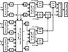 |
Figure 4. Binaural HASPI block diagram showing the time-frequency envelope analysis incorporating the model of binaural interaction. The model includes the amplitude adjustment of the left and right ear signal envelopes to maximize the cross-correlation of the weighted sum with the reference signal envelope. |
Characteristics of the ten filters implemented in the modulation filterbank.
The remaining steps in the modulation analysis are identical with those used for HASPI v2, and the reader is referred to [2] for a complete description. At each time sample at the 2560 Hz sampling rate, the dB envelope values in the 32 frequency bands give the log spectrum on an auditory frequency scale [49]. These auditory spectra are fitted with a set of five basis functions ranging from ½ cycle per spectrum to 2½ cycles per spectrum; these basis functions correspond to mel-frequency cepstral coefficients [62] and also to the principal components of speech short-time spectra [63]. The basis function sequences are then pruned to remove pauses in the speech. Each of the five pruned sequences of cepstral coefficients is passed through a modulation filterbank. There are ten filters in the filterbank; the filter characteristics are shown in Table 1. The filters have Q values of 1.5, which are consistent with the Q values between 1 and 2 that have been fitted to amplitude modulation discrimination data[64, 65].
The envelope modulation filter analysis produces a total of 50 output envelope sequences: five cepstral coefficient sequences each filtered through the ten modulation filters. Cross-covariance is used to compare each of these 50 filtered sequences for the left+right sum to the corresponding sequences for the reference. The basis function cross-correlations are similar to one another [66], so the cross-covariance functions are averaged over the five basis functions to produce an output vector comprising the averaged cross-covariances for each of the ten envelope modulation filters.
3.4. Neural network ensemble
The final processing stage for the binaural HASPI is an ensemble of ten neural networks that map the averaged modulation filter outputs to the subject sentence intelligibility scores. The configuration and design procedure used for the binaural HASPI ensemble of neural networks is identical to that used for the monaural HASPI v2 [2], but the networks here are fitted to the binaural intelligibility data. Each neural network in the ensemble has 10 inputs (the modulation filter outputs), a hidden layer comprising 4 neurons, and an output layer comprising a single neuron. A sigmoid activation function is used for all layers. The ten networks were each initialized to a different independent set of random weights, and network training used backpropagation with a mean-squared error loss function [67]. A total of 16 200 training vectors were available to train the neural networks, with each vector comprising the subject sentence correct score (0 or 1) and the set of averaged modulation filter outputs for the ten modulation filter bands computed for the 540 sentences heard by each of the 15 NH and 15 HIsubjects.
Ensemble averaging was implemented to reduce the possibility of overfitting the data. Bootstrap aggregation [68] was used to combine the outputs from the neural networks. Each neural network was trained using a subset of the 16 200 possible training vectors, with each subset comprising (1 − 1/e)=0.632 of the available data, selected with replacement. Each neural network was trained on 1000 iterations of its randomly selected binaural data subset. An ensemble comprising ten networks was chosen since a group that size provides the main benefits of bootstrap aggregation in reducing overfitting[68, 69].
4. Results
4.1. Audiogram scale factor
The binaural HASPI metric includes the audiogram scale factor described in the Binaural Modifications section above. The audiogram scale factor, although not needed for monaural stimulus presentation, is expected to be relevant for modeling binaural intelligibility for any system using the HASPI or a similar peripheral model. To investigate this hypothesis, the audiogram scale factor was applied to three binaural intelligibility prediction models based on the HASPI peripheral framework.
The simplest modeling approach is to add the audiogram scale factor to the existing HASPI v2, thus increasing the bandwidth of the HI monaural auditory filters while making no other changes to the HASPI v2 intelligibility calculation. This monaural metric was converted into a better ear value by first computing HASPI v2 separately for the left and right ears for all stimulus presentations. The higher of the left-ear and right-ear HASPI values were then selected across the presentations to give the better-ear values. These better-ear HASPI v2 values were then averaged over subject and repetition for each processing condition, producing 54 averaged stimulus condition intelligibility predictions. The RMS error and Pearson correlation coefficient between the averaged better-ear HASPI predictions and the subject intelligibility scores were then computed over the 54 conditions. This procedure was repeated for each of the audiogram scale factors. This modeling approach is denoted as “v2 Better Ear”.
The second model starts with the left and right ear monaural HASPI v2 envelope modulation features calculated using the broadened HI auditory filters as described in the paragraph above. However, separate ensembles of neural networks were computed for the sets of left-ear and right-ear modulation features and each ensemble was fitted to the binaural intelligibility scores. The higher of the computed left and right ear values for each stimulus presentation were then selected and averaged over repetition and subject. This modeling approach is denoted as “Bin Data Better Ear”.
The final approach applies the audiogram scale factor to the peripheral models, but this time followed by the binaural interaction processing stage. The binaural interaction adjusts the time delays and amplitudes between the left and right ear envelopes to maximize the cross-correlation between each ear and the reference and then sums the adjusted left and right ear signals. The envelope modulation correlations obtained using this combined signal are then fitted to the binaural intelligibility scores using an ensemble of neural networks. This third approach is the procedure proposed for the binaural HASPI metric, and is denoted by “Binaural Sum”.
The results plotted in Figure 5 show the RMS error (a) and Pearson correlation coefficient (b) for predicted binaural intelligibility compared to the subject responses for the three models as the audiogram scaling factor was increased from 1 (audiogram used without modification) to 2 (hearing loss doubled in dB at all audiometric frequencies). HASPI v2 fitted to the monaural data (v2 Better Ear) gives the greatest RMS error for audiogram scale factors below 1.50, while fitting the same envelope modulation features to the binaural intelligibility scores (Bin Data Better Ear) greatly reduces the RMS error for audiogram scale factors over this range. The HASPI v2 better-ear (v2 Better Ear) and the better-ear fit to the binaural data (Bin Data Better Ear) show a decrease in RMS error over the audiogram scale factor range of 1–1.67, while the binaural sum model (Binaural Sum) shows decreasing RMS error as the audiogram scale factor increases from 1 to 1.50. The Binaural Sum model shows lower RMS error than either of the models lacking the binaural interaction stage for all audiogram scale factors except for the extremum of 2. The minimum binaural sum RMS error of 0.0493 occurs for an audiogram scale factor of 1.50; this audiogram scale factor was therefore chosen for the implementation of the binaural HASPI. The other two models also show minima in the RMS error, but occurring at audiogram scale factors of1.67 or 2.00.
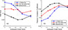 |
Figure 5. RMS binaural intelligibility prediction error (a) and Pearson correlation coefficient (b) for the better-ear monaural HASPI v2 with the neural networks fitted to the monaural intelligibility scores (v2 Better Ear), the better-ear monaural HASPI v2 with the neural networks fitted to the binaural intelligibility scores (Bin Fit Better Ear), and the binaural interaction model fitted to the binaural intelligibility scores (Binaural Sum). The model accuracy is indicated for the combined NH plus HI subjects; each point represents data averaged over processing conditions, subjects, and repetitions. |
The correlation coefficients tend to inversely mirror the RMS error. For all three models the correlation increases monotonically as the audiogram scale factor increases from 1 to 1.67; the binaural interaction model has the highest correlations over this range while the v2 better ear has the lowest. All three models have a maximum correlation peak at the audiogram scale factor of 1.67, although the difference for the binaural sum curve between 1.50 and 1.67 is quite small. Note that the correlation coefficients measure the degree to which theintelligibility scores are linear transformations of the model predictions; the correlations are immune to shifts or biases in the predictions or to differences in the slopes. The RMS error includes both factors and for this reason is our preferred criterion for selecting the audiogram scale factor for the binaural interaction system.
In summary, increasing the audiogram scale factor tends to reduce the RMS error and increase the correlation for all three modeling approaches considered in this section. Futhermore, the binaural interaction model proposed in this paper further reduces the RMS error and increases the correlation coefficient beyond the reduction provided just by increasing the audiogram scale factor, so the benefits of applying both the audiogram scale factor and the binaural interaction model appear to beadditive.
4.2. Monaural HASPI v2 and binaural HASPI for binaural data
This section provides an analysis of the improvement in prediction accuracy offered by the proposed binaural HASPI as contrasted with the existing HASPI v2. The HASPI v2 procedure is the same better-ear calculation as used for evaluating the audiogram scale factor in the section above, with the audiogram scale factor set to 1 to give the conventional HASPI v2 peripheral model and with the neural networks fitted to the monaural data. The binaural HASPI values were computed using the optimal audiogram scale factor of 1.5 determined above and with the binaural interaction procedure described in the Intelligibility Metric section, and the neural networks were fitted to the binaural data.
The scatterplot for the better-ear monaural HASPI v2 values plotted against the subject binaural sentence intelligibility scores is presented in Figure 6a, and the binaural HASPI scatterplot for the binaural data is presented in Figure 6b. The NH subject group is identified by open circles, while the HI group is identified by filled squares. The diagonal lines in the two figures represent perfect performance; a point below the line indicates that the predicted intelligibility is higher than the observed score, while a point above the diagonal indicates that the predicted intelligibility is lower than observed. Points close to the diagonal line indicate a low error, while points arrayed along a line, even if not congruent with the diagonal, indicate a high Pearson correlation coefficient. The RMS error and correlations (Pearson, Spearman rank order, and Kendall’s tau based on pairwise comparisons) corresponding to the data in Figure 6 are presented in Table 2.
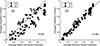 |
Figure 6. Scatterplots comparing (a) better-ear HASPI v2 predictions to the binaural subject intelligibility scores using an audiogram scale factor of 1, and (b) binaural HASPI predictions to the binaural subject intelligibility scores using an audiogram scale factor of 1.5. Each point represents the data for a single processing condition averaged over repetitions and either NH or HI subjects for that condition. Data for the NH subjects are plotted using open circles and data for the HI subjects are plotted using filled squares. |
RMS error and correlations between the model predictions and the subject responses for the better-ear monaural HASPI v2 model with its audiogram scale factor set to 1 and the binaural sum HASPI model with its audiogram scale factor set to 1.5. The data are averaged over subjects and repetitions for each hearing group.
Significant differences between the two subject groups for a given intelligibility model and between models for a given subject group were determined using bootstrapping [68–70]. Group or model differences for 20 000 replications with resampling of the selected comparison (RMS error or correlation criterion) were used to provide confidence limits from which the statistical significance was estimated. Bonferroni adjustments were applied formultiplicity.
In Figure 6a, the HI data lie below but roughly parallel to the NH data. The NH to HI comparisons do not show significant differences for Pearson, Spearman, or Kendall’s tau correlations. However, the RMS error is significantly larger (p < 0.001) for the HI subjects than for the NH subjects. The results for the binaural model are presented in Figure 6b. The HI and NH data now overlap. No significant differences are found for any of the three correlation calculations or for the RMS error, so the binaural model, with its audiogram scale factor, binaural interaction, and fitting to the binaural data, has successfully reduced the RMS error.
The intelligibility models can also be compared for each of the two subject groups. For the NH group, the binaural model has significantly higher Pearson correlation (p = 0.012) than the better-ear model and significantly lower RMS error (p < 0.001). For the HI group, no significant differences were found for any of the three correlation procedures, but, as illustrated in Figure 6b, the binaural model yields significantly lower RMS error (p < 0.001).
5. Discussion
5.1. Comparison to other modeling approaches
Processing, stimuli, and Pearson correlation coefficient results for several existing binaural intelligibility models are summarized in Table 3. Note that it is difficult to compare different binaural intelligibility metrics since not all tested HI subjects and the target speech, noise and interference, HA processing, acoustic environments, and intelligibility criteria varied across studies. Furthermore, most of the models were fitted to the specific data cited in the respective papers and may not be as accurate for different datasets. Despite these caveats, the accuracy of the binaural HASPI, with Pearson correlation coefficients of 0.982, 0.981, and 0.983 for the NH, HI, and combined NH + HI subjects, respectively, compares quite favorably with these previously published results. Even the better-ear HASPI v2, which was trained on monaural headphone data, produces respectable correlation values of 0.961, 0.972, and 0.887 for NH, HI, and NH + HI subjects, respectively. The largest difference in accuracy occurs for the binaural HASPI compared to the models of [23, 24]. However, both these studies evaluated their intelligibility models with the CPC1 dataset; there was no averaging over stimulus repetitions for a given subject or over subject responses for the same stimulus across subjects. The difference in the correlation coefficients could thus be primarily due to greater individual and stimulus variability in the unaveraged responses.
Representative binaural speech intelligibility model results. Abbreviations introduced in this table: Intelligibility (Intel.), Speech-shaped noise (SSN), Ideal Binaural Mask (IBM), International Speech Test Signal (ISTS), Reverberation Time (RT), Clarity Prediction Challenge 1 (CPC1).
The high accuracy for the binaural HASPI indicates that the EC model of binaural interaction is not a requirement for building an accurate binaural metric. The first six models in Table 3 all use EC followed by a monaural metric, but the HASPI approach of independentleft- and right-ear peripheral models followed by a cross-correlation model of binaural interaction appears to work just as well.
5.2. HI bias
The significantly higher RMS error shown in Figure 6a, combined with no significant differences in correlations, indicated a substantial bias for the better-ear HASPI v2 approach: The HI subject sentence intelligibility was consistently predicted to be too high. Existing binaural intelligibility models have shown similar biases. For example, the study reported in [11] used the same model for NH and HI subjects; hearing loss was modeled as an additive internal noise in the EC model and in the SII calculation. Their speech reception threshold (SRT) predictions were underestimated (intelligibility over-estimated) for HI subjects, with errors as large as −5 dB in the SRT predicted for an anechoic room. The study reported in [12] extended the previous model [11] for modulated noises. In the revised model, they found an SRT bias for both NH and HI subjects. The overall bias across hearing groups was −3.4 dB, and the magnitude of the bias for the HI group was equal to or greater than that for the NH group for all rooms, speech and noise azimuths, and noise types. The RMS error in the SRT was 1.3 dB for the NH subjects and was 1.9 dB for the HI subjects. In the study reported in [71], using the Beutelmann and Brand model [12], the authors found thataudiograms alone were insufficient to accurately predict individual SRTs. Prediction accuracy was improved when the individual audiogram was combined with SII calibration using the measured individual SRT for a baseline test condition. The calibration was likened to the use of a proficiency factor in the calculation of the SII [72, 73] that reduces the calculated SII values based on individual intelligibility data.
The HI bias can be reduced when separate models are derived for the NH and HI groups; the separate models may indirectly compensate for changes in binaural processing in the impaired as opposed to the normal periphery. The model proposed in [74] represents hearing loss as an internal noise spectrally shaped to correspond with the individual audiogram which is then adjusted in amplitude using different gains for the NH and HI groups. This procedure for calibrating the SRTs effectively eliminates the HI bias but yields two separate models, one for NH and one for HI subjects. The study of [26] improved upon this model by using an internal noise that separates the estimated influences of inner and outer hair cell losses and which is dependent on the level of the external stimuli. These changes allowed predictions of NH and HI SRTs with a single model without any prediction bias. The model in [75] further refined this approach to predict individual differences among HI SRTs for a given test condition.
The HI bias present in the better-ear HASPI v2 was greatly reduced in the binaural HASPI by multiplying the audiogram in dB by an audiogram scale factor of 1.5, adding the model of binaural interaction, and fitting the model to the binaural data. The remainder of the underlying left and right ear peripheral models are the same as used for the monaural HASPI v2. Scaling the audiogram broadened the auditory filters and shifted the auditory threshold for the HI subjects. It is possible that these changes in the peripheral behavior represent aspects of the auditory efferents and binaural interaction that are not directly included in the binaural HASPI model. The effective auditory bandwidth, for example, is influenced by auditory cross-correlation [76, 77] and interaural modulation processing [78], and auditory gain is reduced by preceding signals activating the efferent system [79, 80]. Modeling the auditory efferents to produce a more accurate model of binaural interaction could potentially lead to a more physiologically valid binaural intelligibility metric. However, the results presented in this paper suggest that modifying the auditory periphery to provide more hearing loss than indicated by the audiogram may be a simple but effective way to improve the accuracy of binaural intelligibility models.
5.3. Limitations
The presentation level used for the speech stimuli was 65 dB SPL for the NH subjects and 65 dB SPL plus compensation for the hearing loss for the HI subjects. However, the gains and auditory filter bandwidths in the HASPI peripheral model depend on the signal intensity, and this level dependence could interact with the proposed audiogram scaling for the hearing loss. For speech at levels greater than the 65 dB SPL used in this paper, the peripheral model will increase the signal levels in each frequency band relative to auditory threshold, with the amount of increase depending on the OHC compression ratio, and will also increase the auditory filter bandwidths. The increased signal level could improve audibility for the HI subjects since more of the speech will fall above the impaired threshold, which would be expected to improve speech intelligibility. However, the broader auditory filter bandwidths will provide greater spectral smoothing that can reduce the cepstral correlation values used to compute the HASPI speech features. The increased signal level thus produces audibility and auditory filter effects that work in opposition. For speech intensities below 65 dB SPL the audibility and auditory filter bandwidth effects are reversed, causing lower audibility combined with improved short-time spectral contrast. It is possible that the magnitude of these stimulus intensity effects could be affected by the audiogram scaling proposed for binaural HASPI, and further investigation of the impact of stimulus intensity is warranted.
6. Conclusions
The goal of this paper was to develop a new version of HASPI that is accurate for binaural speech intelligibility. The starting point for the binaural HASPI was HASPI v2, which was derived for monaural headphone presentation. That model was fitted to a wide range of speech stimuli including additive noise, reverberation, nonlinear distortion, and hearing-aid processing. HASPI v2 incorporates a peripheral model that can be adjusted in response to the subject’s audiogram, making HASPI v2 appropriate for both NH and HI subjects.
The binaural HASPI uses the HASPI v2 peripheral models for the left and right ears. Three modifications were made for predicting binaural intelligibility data. It was found that using the peripheral models as originally developed led to overestimation of the HI speechintelligibility for better-ear monaural predictions; this estimation bias was greatly reduced by multiplying the subject’s audiogram in dB by an audiogram scale factor of 1.5 while keeping the rest of the peripheral model as originally designed. The second modification was the addition of the binaural interaction stage where the left and right ear envelopes are temporally aligned with the center-front anechoic reference and the gains of the aligned left and right ear signals are adjusted to maximize the cross-correlation of the weighted sum with the reference. The final stages of the binaural HASPI then follow the same procedure as used for HASPI v2; the time-frequency envelope modulation extracted from the degraded stimulus summed across the two ears is compared to that of the reference and the sentence intelligibility is estimated using an ensemble of neural networks. The third modification was generating a new ensemble of neural networks based on fitting the binaural HASPI model to the binaural intelligibility data considered in this paper. The binaural HASPI results show that its RMS error and correlation with measured data are comparable to those for previously developed binaural metrics, and that the accuracy for HI subjects is similar to that for NH subjects.
Funding
The authors were supported by a research grant to the University of Colorado from GN ReSound.
Conflicts of interest
The authors declare that they have no conflicts of interest.
Data availability statement
The MATLAB code for the binaural HASPI is available on request from the authors. The stimulus sound files and the subject responses used for this paper are available in the Open Science Framework (OSF) public-domain repository, under the reference https://osf.io/nf23j (NH data) and https://osf.io/yz64u (HI data).
References
- J.M. Kates, K.H. Arehart: The hearing-aid speech perception index (HASPI). Speech Communication 65 (2014) 75–93. [Google Scholar]
- J.M. Kates, K.H. Arehart: The hearing-aid speech perception index (HASPI) version 2. Speech Communication 131 (2021) 35–46. [Google Scholar]
- J.M. Kates, K.H. Arehart: An overview of the HASPI and HASQI metrics for predicting speech intelligibility and speech quality for normal hearing, hearing loss, and hearing aids. Hearing Research 426 (2022) 108608. [Google Scholar]
- A.W. Bronkhorst, R. Plomp: The effect of head-induced interaural time and level differences on speech intelligibility in noise. The Journal of the Acoustical Society of America 83 (1988) 1508–1506. [CrossRef] [PubMed] [Google Scholar]
- J.F. Culling, M.L. Hawley, R.Y. Litovsky: The role of head-induced interaural time and level differences in the speech reception threshold for multiple interfering sound sources. The Journal of the Acoustical Society of America 116 (2004) 1057–1065. [Google Scholar]
- M. Lavandier, J.F. Culling: Prediction of binaural speech intelligibility against noise in rooms. The Journal of the Acoustical Society of America 127 (2010) 387–399. [CrossRef] [PubMed] [Google Scholar]
- N.I. Durlach: Equalization and cancellation theory of binaural masking-level differences. The Journal of the Acoustical Society of America 35 (1963) 1206–1218. [CrossRef] [Google Scholar]
- N.I. Durlach: Binaural signal detection: equalization and cancellation theory, in: Foundations of Modern Theory Vol. II, J.V. Tobias, ed. Academic, New York, 1972. [Google Scholar]
- L.R. Bernstein, C. Trahiotis: An interaural-correlation-based approach that accounts for a wide variety of binaural detection data. The Journal of the Acoustical Society of America 141 (2017) 1150–1160. [Google Scholar]
- ANSI: Methods for the calculation of the Speech Intelligibility Index. Am. Nat. Std. Inst. S3.5-1997 (1997) Approved 6 June 1997. [Google Scholar]
- R. Beutelmann, T. Brand: Prediction of speech intelligibility in spatial noise and reverberation for normal-hearing and hearing-impaired listeners. The Journal of the Acoustical Society of America 120 (2006) 331–342. [CrossRef] [PubMed] [Google Scholar]
- R. Beutelmann, T. Brand, B. Kollmeier: Revision, extension, and evaluation of a binaural speech intelligibility model. The Journal of the Acoustical Society of America 127 (2010) 2479–2497. [CrossRef] [PubMed] [Google Scholar]
- R. Wan, N.I. Durlach, H.S. Colburn: Application of an extended equalization-cancellation model to speech intelligibility with spatially distributed maskers. The Journal of the Acoustical Society of America 128 (2010) 3678–3690. [CrossRef] [PubMed] [Google Scholar]
- C.F. Hauth, S.C. Berning, B. Kollmeier, T. Brand: Modeling binaural unmasking of speech using a bind binaural processing stage. Trends in Hearing 24 (2020) 1–16. [Google Scholar]
- C.H. Taal, R.C. Hendriks, R. Heusdens, J. Jensen: An algorithm for intelligibility prediction of time-frequency weighted noisy speech. IEEE Transactions on Audio, Speech, and Language Processing 19 (2011)2125–2136. [CrossRef] [Google Scholar]
- A.H. Andersen, J.M. de Haan, Z.-H. Tan, J. Jensen: Predicting the intelligibility of noisy and nonlinearly processed binaural speech. IEEE Transactions on Audio, Speech, and Language Processing 24 (2016) 1908–1920. [Google Scholar]
- A.H. Andersen, J.M. de Haan, Z.-H. Tan, J. Jensen: Refinement and validation of the binaural short time objective intelligibility measure for spatially diverse conditions. Speech Communication 102 (2018) 1–13. [Google Scholar]
- A. Chabot-Leclerc, E.N. MacDonald, T. Dau: Predicting binaural speech intelligibility using the signal-to-noise ratio in the envelope power spectrum domain. The Journal of the Acoustical Society of America 140 (2016) 192–205. [Google Scholar]
- T. Biberger, S.D. Ewert: Towards a simplified and generalized monaural and binaural auditory model for psychoacoustics and speech intelligibility. Acta Acustica 6 (2022) 23. [CrossRef] [EDP Sciences] [Google Scholar]
- S.D. Ewert, W. Schubotz, T. Brand, B. Kollmeier: Binaural masking release in symmetric listening conditions with spectro-temporally modulated maskers. The Journal of the Acoustical Society of America 142 (2017) 12–28. [CrossRef] [PubMed] [Google Scholar]
- H.J.M. Steeneken, T. Houtgast: A physical method for measuring speech-transmission quality. The Journal of the Acoustical Society of America 67 (1980) 318–326. [CrossRef] [PubMed] [Google Scholar]
- S.J. van Wijngaarden, R. Drullman: Binaural intelligibility prediction based on the speech transmission index. The Journal of the Acoustical Society of America 123 (2008) 4514–4523. [Google Scholar]
- B.A. Titalim, C.O. Mawalim, S. Okada, M. Unoki: Speech intelligibility prediction for hearing aids using an auditory model and acoustic parameters, in: Proceedings of 2022 Asia-Pacific Signal and Information Processing Association Annual Summit and Conference, Nov. 7–10, Chiang Mai, 2022, pp. 1077–1085. [Google Scholar]
- C.O. Mawalim, B.A. Titalim, M. Unoki, S. Okada: OBISHI: Objective binaural intelligibility score for the hearing impaired, in: Proceedings of 18th Australasian International Conference of Speech Science and Technology, December 13–16, 2022, pp. 111–115. [Google Scholar]
- M. Lavandier, S. Jelfs, J.F. Culling, A.J. Watkins, A.P. Raimond, S.J. Makin: Binaural prediction of speech intelligibility in reverberant rooms with multiple noise sources. The Journal of the Acoustical Society of America 131 (2012) 218–231. [CrossRef] [PubMed] [Google Scholar]
- T. Vicente, M. Lavandier: Further validation of a binaural model predicting speech intelligibility against envelope-modulated noises. Hearing Research 390 (2020) 107937. [CrossRef] [PubMed] [Google Scholar]
- T. Vicente, M. Lavandier, J. Buchholz: A binaural model implementing an internal noise to predict the effect of hearing impairment on speech intelligibility in non-stationary noises. The Journal of the Acoustical Society of America 148 (2020) 3305–3317. [CrossRef] [PubMed] [Google Scholar]
- J.M. Kates: Cross-correlation procedures for measuring noise and distortion in AGC hearing aids. The Journal of the Acoustical Society of America 107 (2000) 3407–3141. [Google Scholar]
- J.M. Kates, M. Lavandier, R.K. Muralimanohar, E.M.H. Lundberg, K.H. Arehart: Binaural speech intelligibility for combinations of noise, reverberation, and hearing-aid signal processing. PLOS One 20 (2025) e0317266. [Google Scholar]
- J.B. Allen, D.A. Berkley: Image method for efficiently simulating small-room acoustics. The Journal of the Acoustical Society of America 65 (1979) 943–950. [Google Scholar]
- J.M. Kates, E.J. Brandewie: Adding air absorption to simulated room acoustic models. The Journal of the Acoustical Society of America 148 (2020) EL408–EL413. [Google Scholar]
- M.D. Burkhard, R.M. Sacks: Anthropometric manikin for acoustic research. The Journal of the Acoustical Society of America 58 (1975) 214–222. [Google Scholar]
- K.H. Arehart, E. Lundberg, S.-H. Chon, L.O. Harvey Jr, J.M. Kates, M.C. Anderson, V.H. Rallapalli, P.E. Souza: A comparison of speech intelligibility and subjective quality with hearing-aid processing in older adults with hearing loss. International Journal of Audiology 61 (2022) 46–58. [Google Scholar]
- J.M. Kates: Modeling the effects of single-microphone noise suppression. Speech Communication 90 (2017) 15–25. [Google Scholar]
- D. Byrne, H. Dillon: The National Acoustic Laboratories’ (NAL) new procedure for selecting the gain and frequency response of a hearing aid. Ear and Hearing 7 (1986) 257–265. [Google Scholar]
- G. Keidser, H. Dillon, M. Flax, T. Ching, S. Brewer: The NAL-NL2 prescription procedure. Audiology Research 1 (2011) e24. [CrossRef] [PubMed] [Google Scholar]
- P.E. Souza, K.H. Arehart, J.M. Kates, N.B.H. Croghan, N. Gehani: Exploring the limits of frequency lowering. Journal of Speech, Language, and Hearing Research 56 (2013) 1349–1363. [Google Scholar]
- J.M. Kates: The electroacoustic system, in: Digital Hearing Aids. San Diego, Plural, 2008, pp. 51–74. [Google Scholar]
- V.H. Rallapalli, A. Mueller, R. Appleton, P.E. Souza: Survey of hearing aid signal processing features across manufacturers, in: Presented at the American Academy of Audiology 2018, Nashville, TN, 2018. [Google Scholar]
- E.H. Rothauser: IEEE recommended practice for speech quality measurements. IEEE Transactions on Audio and Electroacoustics 17 (1969) 225–246. [Google Scholar]
- L.M. Panfili, J. Haywood, D.R. McCloy, P.E. Souza, R.A. Wright: The UW/NU Corpus, Version 2.0 (1987). https://depts.washington.edu/phonlab/projects/uwnu.php. [Google Scholar]
- R.M. Cox, G.C. Alexander, C. Gilmore: Development of the Connected Speech Test (CST). Ear and Hearing 5 (1987) 119S–126S. [Google Scholar]
- K. Smeds, F. Wolters, M. Rung: Estimation of signal-to-noise ratios in realistic sound scenarios. Journal of the American Academy of Audiology 26 (2015) 183–196. [CrossRef] [PubMed] [Google Scholar]
- J.M. Kates: An auditory model for intelligibility and quality predictions, in: Proceedings of Meetings on Acoustics. 165th Meeting. Acoustical Society of America, Montreal June 2–7. Vol. 19, 2013, p. 050184. [Google Scholar]
- J.M. Kates: A time domain digital cochlear model. IEEE Transactions on Signal Processing 39 (1991) 2573–2592. [Google Scholar]
- M. Cooke: Modelling Auditory Processing and Organization. Cambridge University Press, Cambridge UK, 1993. [Google Scholar]
- R.D. Patterson, M.H. Allerhand, C. Giguère: Time-domain modeling of peripheral auditory processing: a modular architecture and a software platform. The Journal of the Acoustical Society of America 98 (1995) 1890–1894. [CrossRef] [PubMed] [Google Scholar]
- B.C.J. Moore, D.A. Vickers, C.J. Plack, A.J. Oxenham: Inter-relationship between different psychoacoustic measures assumed to be related to the cochlear active mechanism. The Journal of the Acoustical Society of America 106 (1999) 2761–2778. [Google Scholar]
- B.C.J. Moore, B.R. Glasberg: Suggested formulae for calculating auditory-filter bandwidths and excitation patterns. The Journal of the Acoustical Society of America 74 (1999) 750–753. [Google Scholar]
- R.J. Baker, S. Rosen: Auditory filter nonlinearity in mild/moderate hearing impairment. The Journal of the Acoustical Society of America 111 (2002) 1330–1339. [Google Scholar]
- R.J. Baker, S. Rosen: Auditory filter nonlinearity across frequency using simultaneous notch-noise masking. The Journal of the Acoustical Society of America 119 (2006) 454–462. [Google Scholar]
- M.A. Ruggero, N.C. Rich, A. Recio, S. Narayan, L. Robles: Basilar-membrane responses to tones at the base of the chinchilla cochlea. The Journal of the Acoustical Society of America 101 (1997) 2151–2163. [Google Scholar]
- X. Zhang, M.G. Heinz, I.C. Bruce, L.H. Carney: A phenomenological model for the response of auditory nerve fibers: I. Nonlinear tuning with compression and suppression. The Journal of the Acoustical Society of America 109 (2001) 648–670. [Google Scholar]
- D.M. Harris, P. Dallos: Forward masking of auditory nerve fiber responses. Journal of Neurophysiology 42 (1979) 1083–1107. [CrossRef] [PubMed] [Google Scholar]
- M. Wojtczak, J.A. Biem, C. Micheyl, A.J. Oxenham: Perception of across-frequency asynchrony and the role of cochlear delay. The Journal of the Acoustical Society of America 131 (2012) 363–377. [Google Scholar]
- M. Nitschmann, J.L. Verhey, B. Kollmeier: Monaural and binaural frequency selectivity in hearing-impaired subjects. International Journal of Audiology 49 (2010) 357–367. [PubMed] [Google Scholar]
- A.J. Kolarik, J.F. Culling: Measurement of the binaural auditory filter using a detection task. The Journal of the Acoustical Society of America 127 (2010) 3009–3017. [Google Scholar]
- J. Breebart, S. van de Par, A. Kohlrausch: Binaural processing model based on contralateral inhibition. II. Dependence on spectral parameters. The Journal of the Acoustical Society of America 110 (2001) 1089–1104. [Google Scholar]
- J.M. Kates: Understanding compression: modeling the effects of dynamic-range compression in hearing aids. International Journal of Audiology 49 (2010) 395–409. [CrossRef] [PubMed] [Google Scholar]
- V.P. Sivonen: Directional loudness and binaural summation for wideband and reverberant sounds. The Journal of the Acoustical Society of America 121 (2007)2852–2861. [Google Scholar]
- B.C.J. Moore, M. Jervis, L. Harries, J. Schlittenlacher: Testing and refining a loudness model for time-varying sounds incorporating binaural inhibition. The Journal of the Acoustical Society of America 143 (2018) 1504–1513. [Google Scholar]
- V. Mitra, H. Franco, M. Graciarena, A. Mandal: Normalized amplitude modulation features for large vocabulary noise-robust speech recognition, in: Proceedings of IEEE International Conference on Acoustics, Speech and Signal Processing. Kyoto, March 25–30, 2012, pp. 4117–4120. [Google Scholar]
- S.A. Zahorian, M. Rothenberg: Principal-components analysis for low-redundancy encoding of speech spectra. The Journal of the Acoustical Society of America 69 (1981) 832–845. [Google Scholar]
- S.D. Ewert, T. Dau: Characterizing frequency selectivity for envelope fluctuations. The Journal of the Acoustical Society of America 108 (2000) 1181–1196. [Google Scholar]
- S.D. Ewert, J.L. Verhey, T. Dau: Spectro-temporal processing in the envelope-frequency domain. The Journal of the Acoustical Society of America 112 (2002)2921–2931. [Google Scholar]
- J.M. Kates, K.H. Arehart: Comparing the information conveyed by envelope modulation for speech intelligibility, speech quality, and music quality. The Journal of the Acoustical Society of America 138 (2015) 2470–2482. [Google Scholar]
- D.E. Rumelhart, G.E. Hinton, R.J. Williams: Learning internal representations by error propagation, in: Parallel Distributed Processing, D.E. Rumelhart, J.L. McClelland, eds. Vol. 1. MIT Press, Cambridge MA, USA, 1986. [Google Scholar]
- L. Breiman: Bagging predictors. Machine Learning 24 (1996) 123–140. [Google Scholar]
- L.K. Hansen, P. Salamon: Neural network ensembles. IEEE Transactions on Pattern Analysis and Machine Intelligence 12 (1990) 993–1001. [Google Scholar]
- B. Efron: Estimating the error rate of a prediction rule: improvement on cross-validation. Journal of the American Statistical Association 78 (1983) 316–331. [Google Scholar]
- A.M. Kubiak, J. Rennies, S.D. Ewert, B. Kollmeier: Prediction of individual speech recognition performance in complex listening conditions. The Journal of the Acoustical Society of America 147 (2020) 1379–1391. [Google Scholar]
- C.V. Pavlovic, G.A. Studebaker, R.L. Sherbecoe: An articulation index based procedure for predicting the speech recognition performance of hearing-impaired individuals. The Journal of the Acoustical Society of America 80 (1986) 50–57. [Google Scholar]
- T.Y.C. Ching, H. Dillon, D. Byrne: Speech recognition of hearing-impaired listeners: predictions from audibility and the limited role of high-frequency amplification. The Journal of the Acoustical Society of America 103 (1998) 1128–1140. [Google Scholar]
- M. Lavandier J.M. Buchholz, B. Rana: A binaural model predicting speech intelligibility in the presence of stationary noise and noise-vocoded speech interferers for normal-hearing and hearing-impaired listeners. Acta Acustica 104 (2018) 909–913. [Google Scholar]
- M. Lavandier C.R. Mason, L.S. Baltzell, V. Best: Individual differences in speech intelligibility at a cocktail party: a modeling perspective. The Journal of the Acoustical Society of America 150 (2021) 1076–1087. [Google Scholar]
- J.L. Verhey, M. Nitschmann: Binaural spectral resolution as a function of interaural masker correlation. The Journal of the Acoustical Society of America 135 (2014) 1993–2001. [Google Scholar]
- B. Eurich, J. Encke, S.D. Ewert, M. Dietz: Lower interaural coherence in off-signal bands impairs binaural detection. The Journal of the Acoustical Society of America 151 (2022) 3927–3936. [Google Scholar]
- J.L. Verhey, S. van de Par: Binaural frequency selectivity in humans. European Journal of Neuroscience 51 (2020) 1179–1190. [Google Scholar]
- J.L. Verhey, M. Kordus, V. Drga, I. Yaslin: Effect of efferent activation on binaural frequency selectivity. Hearing Research 350 (2017) 152–129. [Google Scholar]
- A. Farhadi, S.G. Jennings, E.A. Strickland, L.H. Carney: Subcortical auditory model including efferent dynamic gain control with inputs from cochlear nucleus and inferior colliculus. The Journal of the Acoustical Society of America 154 (2023)3644–3659. [Google Scholar]
Cite this article as: Kates J.M. Lavandier M. Arehart K.H. Lundberg E.M.H. & Muralimanohar R.K. 2025. A binaural implementation of the Hearing Aid Speech Perception Index (HASPI). Acta Acustica, 9, 74. https://doi.org/10.1051/aacus/2025054.
All Tables
RMS error and correlations between the model predictions and the subject responses for the better-ear monaural HASPI v2 model with its audiogram scale factor set to 1 and the binaural sum HASPI model with its audiogram scale factor set to 1.5. The data are averaged over subjects and repetitions for each hearing group.
Representative binaural speech intelligibility model results. Abbreviations introduced in this table: Intelligibility (Intel.), Speech-shaped noise (SSN), Ideal Binaural Mask (IBM), International Speech Test Signal (ISTS), Reverberation Time (RT), Clarity Prediction Challenge 1 (CPC1).
All Figures
|
Figure 1. Audiograms in dB HL for the HI subjects averaged across the two ears. The individual audiograms are indicated by the dashed lines and the group average by the solid black line (from Kates et al. [29]). |
| In the text | |
|
Figure 2. Binaural HASPI block diagram showing the comparison of the left and right ear signals with the reference signal. |
| In the text | |
|
Figure 3. Binaural HASPI block diagram of the auditory model used to extract the signal envelopes in each frequency band. |
| In the text | |
|
Figure 4. Binaural HASPI block diagram showing the time-frequency envelope analysis incorporating the model of binaural interaction. The model includes the amplitude adjustment of the left and right ear signal envelopes to maximize the cross-correlation of the weighted sum with the reference signal envelope. |
| In the text | |
|
Figure 5. RMS binaural intelligibility prediction error (a) and Pearson correlation coefficient (b) for the better-ear monaural HASPI v2 with the neural networks fitted to the monaural intelligibility scores (v2 Better Ear), the better-ear monaural HASPI v2 with the neural networks fitted to the binaural intelligibility scores (Bin Fit Better Ear), and the binaural interaction model fitted to the binaural intelligibility scores (Binaural Sum). The model accuracy is indicated for the combined NH plus HI subjects; each point represents data averaged over processing conditions, subjects, and repetitions. |
| In the text | |
|
Figure 6. Scatterplots comparing (a) better-ear HASPI v2 predictions to the binaural subject intelligibility scores using an audiogram scale factor of 1, and (b) binaural HASPI predictions to the binaural subject intelligibility scores using an audiogram scale factor of 1.5. Each point represents the data for a single processing condition averaged over repetitions and either NH or HI subjects for that condition. Data for the NH subjects are plotted using open circles and data for the HI subjects are plotted using filled squares. |
| In the text | |
Current usage metrics show cumulative count of Article Views (full-text article views including HTML views, PDF and ePub downloads, according to the available data) and Abstracts Views on Vision4Press platform.
Data correspond to usage on the plateform after 2015. The current usage metrics is available 48-96 hours after online publication and is updated daily on week days.
Initial download of the metrics may take a while.