| Issue |
Acta Acust.
Volume 9, 2025
|
|
|---|---|---|
| Article Number | 73 | |
| Number of page(s) | 17 | |
| Section | Hearing, Audiology and Psychoacoustics | |
| DOI | https://doi.org/10.1051/aacus/2025055 | |
| Published online | 27 November 2025 | |
Scientific Article
Methods to experimentally characterize the own-voice-generated objective occlusion effect induced by hearables
1
Institut für Hörtechnik und Audiologie, Jade Hochschule Oldenburg, Ofener Str. 16, 26121 Oldenburg, Germany
2
Cluster of Excellence “Hearing4All”
3
Institute for Hearing Technology and Acoustics, RWTH Aachen University, Aachen, Germany
* Corresponding author: This email address is being protected from spambots. You need JavaScript enabled to view it.
Received:
10
April
2025
Accepted:
16
October
2025
Abstract
In this study, the problem of experimentally identifying the own-voice generated objective occlusion effect in hearables is addressed. Challenges arise from the sub-optimal properties of one’s own voice as a test signal, namely, poor reproducibility, limited bandwidth, and the induction of time-variant behavior of the effect being measured. Based on experiments with 19 participants wearing a vented hearable and producing running speech and a sung vowel, it was found that (a) running speech is better suited than vowels in most respects, except for the time-variance of the occlusion effect, (b) the use of transfer function-based estimates of the occlusion effect results in more problems than advantages in comparison to estimates based on power spectral densities, and (c) the popular method of measuring the occlusion effect by simultaneously measuring inside and outside the occluding device entails systematic errors of up to about 3–4 dB, even in the frequency range in which it was previously considered valid. In contrast, the simultaneous measurement with reference to the open contralateral ear is accurate throughout the frequency range in which an acceptable SNR is achieved.
Key words: Own voice / Objective occlusion effect / Hearables
© The Author(s), Published by EDP Sciences, 2025
 This is an Open Access article distributed under the terms of the Creative Commons Attribution License (https://creativecommons.org/licenses/by/4.0), which permits unrestricted use, distribution, and reproduction in any medium, provided the original work is properly cited.
1 Introduction
The alteration of one’s own voice following the insertion of an in-ear hearing device is considered a significant issue in modern hearing technology. By completely or partially obstructing the ear canal, the sound transmission pathways are altered, namely the air-conduction pathways from the mouth through the air into the ear canal, and the bone-conduction pathways where sound is transmitted to the ear canal by vibrations in the bones and tissues of the neck and head [1, 2]. There are also bone-conduction pathways to the middle and inner ears, but they are neglected in the current context. More specifically, occluding devices cause a level increase for bone-conducted sound, especially below 1 kHz, while attenuating the air-conducted sounds at frequencies above [3]. The resulting change in the sound pressure level at the eardrum is commonly known as the objective occlusion effect (OE),
 (1)
(1)
In equation (1),  and
and  are the root mean square values of the eardrum sound pressure in the occluded ear and in the open ear, respectively, see also Figure 1 for an illustration. This effect has been shown to be strongest for closed vowels such as /i:/, whereas it is weaker for open vowels such as /a:/ [3, 4]. In addition, it depends on the insertion depth of the in-ear device [3] and on the contact geometry between device and ear canal walls [5, 6], on the design of the in-ear device [6, 7], and on individual factors such as ear canal geometry and compliance [7–10].
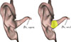 |
Figure 1. Illustration of the occlusion effect: by occluding the ear, the eardrum sound pressure changes from pe, open to pe, occl. |
The own-voice-generated objective occlusion effect has long been identified as one of the most pressing concerns in hearing aids and hearables [7, 11, 12]. Both passive and active measures have been proposed to mitigate the occlusion effect. Passive measures usually comprise vents or open fittings that allow some outward dissipation of bone-conducted sounds. Proper vent sizing allows for better control of the occlusion effect [13], but does not completely mitigate it. Re-opening the ear canal can also cause problems elsewhere by reducing the passive sound insulation of the hearing system, worsening the signal-to-noise ratio (SNR), increasing the risk of feedback at high gain levels, or reducing the effectiveness of adaptive features such as directional microphones or active noise reduction [11, 14, 15].
The advent of hearables, i.e., modern consumer-grade in-ear hearing devices often equipped with multiple sensors, has added new perspectives to occlusion mitigation approaches: hearables are often vented and possess sensors and actuators that enable active approaches where an optimal sound processing for both internal (such as own voice) and external (surrounding the listener) sources is desired. As a result, the frequency range of interest is extended to higher frequencies compared to previous work on occlusion, which mostly focused on low-frequency features and rarely considered frequencies above 2 kHz.
Active Occlusion Cancellation (AOC) has gained traction in recent years as an alternative to passive approaches [16, 17]. For this purpose, hearables often feature multiple microphones inside and outside the ear canal. The goal is to use the microphone signals to accurately predict the open ear sound pressure at the eardrum from the occluded ear measurements. This information will then be used to drive the receivers to ideally restore the eardrum pressure generated by one’s own voice to normal (i.e., the open ear case).
Because of the highly individual nature of the OE, both passive and active approaches would benefit from an accurate individual characterization of the OE. In addition, more accurate measurements may also be helpful to establish correlations between the subjective annoyance and the objectively measured OE. This correlation has often been reported to be weak, see e.g., [7, 18]. However, the accuracy of the objective measurements is usually not questioned.
Determining open and occluded sound pressures in the same ear can only be achieved in a sequential way, i.e., measuring in two trials one after the other. This means that everything must be kept constant across the two trials, except for the insertion of the occluding device. However, own-voice excitation will never be exactly the same in any two trials. One possibility to address this difficulty is to provide real-time feedback to participants regarding the current sound pressure level, to encourage them to maintain a certain level during voice production [19, 20]. Alternatively, a reference sound pressure can be measured by using a second microphone, e.g., in front of the participant [19]. By relating the sound pressures in the open and occluded ear conditions to this reference, one can derive a frequency-dependent correction to compensate for the variability between trials.
In contrast to sequential measurements of the OE, simultaneous measurements circumvent problems related to the variability of own-voice production. One possibility is to measure the sound pressure simultaneously in both ear canals by occluding the ipsilateral ear while leaving the contralateral ear open [20]. Furthermore, when assuming that the sound pressure just outside the occluded ear canal is approximately equal to the sound pressure inside the open ear canal, the sound picked up by a microphone on the outer surface of the occluding device can directly be employed as open ear quantity [21–23]. This approach is valid at lower frequencies and is implemented, e.g., in the Etymotic ER-33 occlusion measurement system [24]. In hearables, the presence of microphones inside and outside the device makes the simultaneous measurement of the occlusion effect particularly appealing.
Saint-Gaudens et al. [20] showed that the sequential approach with participant feedback and the simultaneous measurement with reference to the open contralateral ear provide equivalent occlusion effects. When measuring simultaneously using a microphone just outside the occluding device, equivalence was stated up to approximately 800 Hz. However, these investigations were restricted to frequencies below 2 kHz, and their occluding device did not include vents or openings, as often found in modern hearing devices and hearables.
Furthermore, previous studie s mostly calculated the occlusion effect from power-based quantities, i.e., sound pressure levels or power-spectral densities (PSDs). Since modern hearables provide possibilities to conduct multi-channel measurements, relative transfer functions may be an appealing alternative to PSDs (see Sect. 2), potentially enlarging the frequency range where the estimated OE is not biased by noise in the measured signals.
In clinical settings, occlusion effects are sometimes measured with bone-conduction excitation, e.g., by using tuning forks or bone-conduction transducers on patients’ heads. While this approach can successfully elicit the occlusion effect, the excitation mechanism differs from that of own-voice excitation. In particular, the air-conduction pathway is essentially nonexistent with bone-conduction excitation, unlike with own-voice excitation. Saint-Gaudens et al. [20] showed that excitation with a bone-conduction transducer on the mastoid created occlusion effects similar to those created by mastication, but substantially higher than those created by own-voice excitation. This highlights the necessity of carefully specifying the excitation when measuring the occlusion effect.
With this study, we address the problem of experimentally identifying the own-voice generated objective occlusion effect (OE) in hearables, using participants’ own voices as excitation signals. Specific attention is given to obtaining a wide frequency range and to clarifying the relation between sequential and simultaneous measurements of the OE. Additionally, we investigate the derivation of the OE from both measured power spectral densities (PSDs) and relative transfer functions (TFs). As the occluding device, we use a vented earpiece previously developed for research on assistive hearing devices and hearables [25].
2 Methods
2.1 Signal model
As stated in equation (1), the objective occlusion effect is defined as the sound pressure level difference between the occluded and open ear conditions. These sound pressures can be conceptualized as being produced by the transfer from an unobservable own-voice excitation signal x to the sound pressure pe at the eardrum, see Figure 2. The excitation signal x may be different in every condition. In Figure 2, the transfer from the excitation x to the ear canal pressure pe is represented by the transfer function G, which will also be referred to as “test path" in the following. It is important to note that this transfer function varies between the occluded and open ear conditions. Also, G is not directly observable since x is not observable.
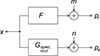 |
Figure 2. Signal model of the objective occlusion effect, including a reference path: x is the unobservable excitation by one’s own voice, which may change in every condition. p r and p e are the reference and eardrum sound pressures, respectively. m and n are uncorrelated noise signals representing background noise and other disturbances on the measured sound pressure signals. |
If a reference sound pressure, denoted by pr, is measured, it can be conceptualized as being produced by an alternative transfer function, designated as F in Figure 2. This (again, unobservable) transfer function will be referred to as “reference path" in the following, and is assumed to remain unchanged with respect to the open or occluded ear conditions. In this study, the measurement of pr will be conducted in either the open contralateral ear or just outside the occluding device.
To account for disturbances on the measured pressure signals, noise signals m and n are added to the outputs of G and F. It is assumed that these noise signals are uncorrelated with each other and with all other signals.
Using the signal model from Figure 2, the occlusion effect can be expressed as
 (2)
(2)
All quantities in equation (2) are frequency dependent, but here and in the following, we omit this dependency for brevity.
Since x will likely change on every voice activity, the measurement of the occluded and open ear conditions must be related to each other. This is accomplished by relating the eardrum to the reference pressure, separately in both conditions. In the ideal undisturbed case, i.e., m = n = 0, this yields
 (3)
(3)
When the occlusion effect is measured simultaneously, the underlying assumption is that the reference path and the test path are equal in the open ear condition,
 (4)
(4)
In this case, equation (3) can be substituted by
 (5)
(5)
2.2 Occlusion effect via power spectral densities (PSDs)
As noted above, neither F nor G is directly observable; therefore, they must be estimated from measurements of the eardrum and reference sound pressures. To obtain spectral representations, power spectral densities (PSDs) of the sound pressures can be used, in both the open and occluded ear conditions in a sequential measurement,
 (6)
(6)
Here, Φee is the PSD of the eardrum sound pressure and Φrr that of the reference sound pressure. Assuming uncorrelated disturbances m and n, the disturbance (noise) PSDs will add to the PSDs at the outputs of F and G,
 (7)
(7)
and the measured occlusion effect will be biased if the signal-to-noise ratio in any of the four sound pressure measurements is low.
In the simultaneous measurement of the occlusion effect with reference to the sound pressure just outside the occluding device, the objective occlusion effect can be estimated as
 (8)
(8)
using PSDs of the eardrum sound pressure and of the sound pressure just outside the occluding device, in the occluded ear condition. Similar to the sequential measurement, this estimate will again be affected by noise PSDs and may hence be biased.
As pointed out in Section 1, one can also use the sound pressure in the open contralateral ear as a reference in simultaneous measurements of the occlusion effect and relate the simultaneously measured sound pressure in the occluded ear to it. In this case, the challenge is to satisfy equation (4) by carefully placing the probe tube microphones as symmetrically as possible in the ipsilateral and contralateral ears. Then,
 (9)
(9)
Equations (6), (7), and (8) describe level differences, in line with the definition of the occlusion effect. Sometimes it is helpful to consider the arguments of the logarithms in these equations, which we will refer to as “occlusion ratios" in the following.
2.3 Occlusion effect via transfer functions (TFs)
In all measurements, ratios of PSDs can be substituted by the square of the absolute value of the transfer function H re of p e, relative to p r, as long as F and G represent linear time-invariant systems. Potentially, this could enlarge the frequency range where the estimated occlusion effect is not biased by Φmm and Φnn, see discussion below. Transfer function-based occlusion effects are defined as
 (10)
(10)
for the sequential case, and as
 (11)
(11)
for the simultaneous cases. Note again that in the simultaneous cases, only the occluded ear condition is considered.
Now, the influence of Φmm and Φnn depends on the choice of a suitable transfer function estimate. For instance, the H 1 estimate
 (12)
(12)
is not biased by Φnn, whereas the H 2 estimate
 (13)
(13)
is not biased by Φmm, see, e.g., Bendat and Piersol [26]. Alternatively, the H V estimate
 (14)
(14)
originally introduced as the H S estimate by Wicks and Vold [27], is optimal if Φmm = Φnn. H 1, H 2 and H V are “classical” TF estimates. A more generalized TF estimate is the H P∞ estimate [28],
 (15)
(15)
where the ratio  is a parameter that is typically chosen to be equal to the ratio of the noise PSDs, i.e.,
 (16)
(16)
Note that with this parameter choice, equation (13) is a special case of equation (14), which occurs when the noise PSDs are equal.
Moreover, the magnitude squared coherence (MSC, γ re 2) between p e and p r,
 (17)
(17)
can be used as a quality indicator. Also, the MSC between the two measured pressure signals is equal to the product of the (unobservable) MSCs of the test path and the reference path [26],
 (18)
(18)
2.4 Participants, occluding device, stimuli, and experimental procedure
The present study involved 19 participants (8 female and 11 male), aged between 21 and 55 years. They were compensated for their participation in this study. 18 of them were native German speakers, and all of them had self-reported normal or near-normal (in one person) hearing. The 20th person had to be excluded because the earmold of the hearing system did not fit reliably into the pinna. In addition, the results for one ear were discarded due to a probe tube microphone malfunction that was not discovered until after the experiment. Therefore, data from 37 ears were analyzed in this study.
The occluding device that was used in this study was designed in a scientific context in order to develop algorithms to improve the sound quality of in-ear hearing systems [25]. It includes four microphones (Knowles type SPH1642HT5H-1, Knowles Electronics, LLC. Itasca, IL, USA) and two receivers, built into a generic ear mold that seals the ear canal with a dome made of silicone. In the present study, only one of the earpiece microphones (“concha mic" at the faceplate of the device) was used, see Figure 3. The earpiece contains a vent that is 19.2 mm long with a cross-section of about 1.5 mm2.
In addition to the hearing device microphone, two probe-tube microphones (type ER-7C Series A and B, Etymotic Research, Elk Grove Village, IL, USA, now discontinued) were used in participants’ ears.
In the experiment, participants were asked to produce various own-voice stimuli, including (a) reading a short German text (“Nordwind und Sonne", text version from the IPA Handbook [29]), and (b) singing each of the five vowels /a:/, /e:/, /i:/, /o:/, /u:/ twice, starting at a low pitch and increasing in pitch as far as possible. Only /i:/ will be analyzed in this work, since it is the vowel known to create the largest occlusion effect [3, 4]. Pitch variation was introduced to close the spectral gap between the fundamental frequency and the formants. To facilitate the tasks, the text was displayed on a screen located at about 1.5 m distance in front of the participants. In addition, an audio example was played before each sung vowel so that participants could get a better understanding of what to produce.
Prior to the actual experiment, participants practiced singing vowels until they felt comfortable with this task. Also, a suitable dome was chosen for the in-ear hearing systems to obtain a reliable fit in the ear canal. The probe-tube microphones were then inserted into both open ears at 2–3 mm distance to the eardrum. The probe tip position was verified using a hand-held otoscope (mini 2000, HEINE Optotechnik, Gilching, Germany). The probe tubes were placed in the incisura intertragica along the lower ear canal wall and secured to the pinna with non-irritating tape to ensure a constant position throughout the experiment.
During the experiment, participants were guided by instructions displayed on the screen in front of them. The experiment included three different conditions, see Figure 4, in each of which all stimuli were produced. In the first condition, both ears were open (top sketch in Fig. 4). For the second and third conditions, the hearing device was inserted into the participant’s left and right ear, respectively, while the probe tube microphones remained in place (middle and bottom sketches in Fig. 4). Note that in these conditions, the probe tube bypassed the earpiece. This way, the best possible reproducibility of the probe tip position across measurement conditions could be obtained. On the other hand, this method may cause problems such as signal attenuation due to squeezed probe tubes and/or additional leaks. However, these issues are minimized by the earpiece’s “one-size-fits-all" design, which creates a seal with the ear canal walls primarily through a soft dome, see Figure 3. Since the dome is much more compliant than the probe tube, the risk of both problems is reduced. Most importantly, if present, both problems will affect all occluded measurements equally. Therefore, they will not influence the results of the present study, which focuses on comparing methods rather than characterizing the occluding device.
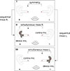 |
Figure 4. Open and occluded ear conditions investigated in this study: (I) both ears open, with probe tube microphones at each eardrum, (II) and (III) one ear occluded, one open, probe tube microphones as in I. |
As indicated in Figure 4, the whole procedure enables a simultaneous and a sequential measurement of the OE for both ears, respectively.
In addition to the own-voice stimuli, excitation via a frontal loudspeaker (Genelec type 8030C, Genelec Oy, Iisalmi, Finland) was used in all three conditions, to measure transfer functions of the eardrum and the earpiece microphone sound pressure, relative to the electrical voltage at the input to the active loudspeaker amplifier.
By relating the transfer functions obtained with loudspeaker excitation in the open ear condition (I in Fig. 4) to that in the occluded ear conditions (II and III in Fig. 4), modified open ear gain functions for external sources are obtained, which can be used to enhance occlusion effects measured with reference to the device microphone, see Section 3.5.
2.5 Recording and microphone calibration
Microphone signal conditioning for the probe tube microphones was provided by the power supplies included with the probe tube systems. For the earpiece microphones, a custom-made power supply was used. The amplified signals were then digitized (24 bit, 44100 Hz sampling rate) using a multi-channel audio interface (ANDIAMO MC, DirectOut GmbH, Mittweida, Germany) that was also used to feed the loudspeaker signal. For the own-voice stimuli, the signal acquisition was controlled via a laptop computer running Matlab version 2021b (The MathWorks, Inc., Natick, MA, USA), using the Audio Toolbox version 2021b. For the loudspeaker transfer functions, signal in- and output was controlled via Pure Data [30] version 0.42, using scripts derived from PureMeasurement [31].
Prior to the experiments, frequency-dependent microphone sensitivities of the probe tube microphones (with tube) were measured in an anechoic room at Jade Hochschule, using the substitution method (DIN EN 61094-8:2013-04) with a free-field reference microphone (GRAS type 40AF + 26AK preamplifier, GRAS Sound & Vibration, Holte, Denmark) and the same loudspeaker model that was also used in the experiments. The earpiece microphones were calibrated using the same technique prior to assembling the earpieces.
2.6 Data processing
2.6.1 Segmenting signals and noise, spectral estimates and frequency-domain smoothing
For further analysis, voice (speech or vowels) and noise parts were extracted manually from the recorded signals by inspection of waveforms and spectrograms. This allowed not only for the separation of voice and noise parts, but also for the rejection of artifacts such as impulsive noises during pauses.
The extracted signals were then used to estimate PSDs separately for voice and noise using Welch’s method [32], and TFs using the TF estimates discussed in Section 2.6.2 below. In all spectral estimates, Hann-windowed time windows of 16 384 samples length and 50% overlap were used. For the sung vowels, recorded pauses were too short for meaningful noise PSD estimates. Therefore, the noise PSD estimates based on pauses between portions of the speech signal that was produced immediately before the vowels were sung are used throughout this work.
Finally, PSD and magnitude squared TF estimates were smoothed into third octave bands using the method of Hatziantoniou and Mourjopoulos [33].
2.6.2 Choice of transfer function estimates
The choice of optimal (i.e., unbiased) TF estimates depends on knowledge of the disturbances m and n. A typical example is shown in Figure 5: The noise PSDs appear to be very similar for both the ipsilateral and the contralateral ear sound pressures in the open ear condition, see column (a). This also applies to the noise PSD in the contralateral (reference) ear when the ipsilateral (test) ear is occluded, but not to the sound pressure in the ipsilateral test ear, see column (b). Since we used the same type of probe microphone in both the ipsilateral and the contralateral ear, this indicates that we essentially observe the microphone self-noise in open ears. The acoustic background noise must be lower, because in column (c), where the device microphone with substantially less self-noise than the probe tube microphones is used, a substantially lower noise PSD is observed (“device noise”). The elevated level of the noise PSD (“ipsi noise”) in the occluded ear condition between 50 Hz and 1200 Hz can be explained by the amplification of bodily sounds such as breathing, which is a known effect ofocclusion.
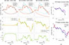 |
Figure 5. Example of measured PSDs, TFs, derived occlusion effects and MSCs in the left ear of one participant producing running speech. Column (a): both ears open (open ear condition in the sequential measurement), column (b): ipsilateral ear occluded (occluded ear condition used in both the sequential and the simultaneous measurements), column (c): same as (b), but the reference changed from the contralateral sound pressure to the ipsilateral sound pressure outside the device (simultaneous measurement), column (d): derived occlusion effects: PSD-based (top) and TF-based (bottom). |
As discussed in Section 2.3, the HV estimate is unbiased for equal noise PSDs. Therefore, we used this estimate to produce TF estimates in the open ear conditions and also in the occluded ear conditions with reference to the contralateral ear sound pressure. In the latter condition, the HV estimate might be sub-optimal since we noted elevated noise PSDs due to bodily sounds in the occluded test ear. However, even with this restriction, the HV estimate seems to be the most reasonable choice among the classical TF estimates.
In the occluded ear condition with reference to the sound pressure outside the occluding device, the noise PSDs are similar at very low frequencies, whereas the noise PSD of the reference signal (sound pressure just outside the occluding device) becomes substantially lower than that of the occluded ear sound pressure with increasing frequency. Hence, the H V estimate would be suited at low frequencies and the H 1 estimate at high frequencies. We finally used a mix of both estimates in this condition, which was formed as follows: At frequencies above 1 kHz, the frequency where the difference between the absolute values of the H V and the H 1 estimate was minimal was identified. This occurred at frequencies between 1066 Hz and 4369 Hz (mean 2773 Hz). At this frequency, we simply shifted from the H V to the H 1 estimate, without applying any frequency-domain cross-fading.
In addition to these classical TF estimates, the H P∞ estimate with the parameter choice from equation (15) was used in all measurements.
2.6.3 Error considerations and valid frequency ranges
2.6.4 (a) Bias and random errors on PSDs
Spectral estimates, such as PSD and TF estimates, contain bias and random errors. If these errors become as large as or even larger than the quantity we aim to measure, the results are no longer reliable. For instance, in the occluded ear condition, one often observes that the measured PSDs are dominated by noise in the occluded test ear at high frequencies above about 3 kHz, see e.g., the diagrams in the top row of Figures 5b and 5c.
Bias errors on PSD estimates are often caused by microphone and/or background noise. If the noise is uncorrelated with the signal, noise compensation can be attempted by subtracting the noise PSD from the PSD measured during voice production. This requires the noise to be stationary. However, even though the noise recordings were carefully segmented to not contain non-stationary components like impulses, breathing and swallowing, see Section 2.6.1, those were clearly present and must be expected to have occurred during voice production as well. Because of these non-stationary effects, we refrained from applying any noise compensation to the measured PSDs.
Instead, we used a requirement on minimum level differences between measurement and noise levels to define valid frequency ranges that were likely not affected by noise-induced bias. More specifically, a minimum level difference of
 (19)
(19)
between the (noise-corrupted) measurement and the noise alone was required to consider the measurement as valid with respect to noise-induced bias.
The variance of the random error of a PSD estimate is, at any frequency away from zero and the Nyquist frequency, given by
 (20)
(20)
assuming that the quantity whose PSD is to be estimated is a sample from a Gaussian process [32]. In equation (19), K is the number of blocks and ρ(k) is the normalized correlation coefficient between blocks that are k D samples apart, where D is the shift (in samples) between successive blocks. By using a 16 384 point Hann time window and 50% overlap (see Sect. 2.6.1), the factor in parentheses is about 1.06, i.e., one can essentially ignore the correlation between successive blocks.
The variance of the PSD estimate will be further reduced by smoothing across frequencies. Since we used smoothing into bands of constant relative bandwidths, the effective number of frequency bins that go into the smoothing is a function of frequency,
 (21)
(21)
Here, b is the relative bandwidth of the smoothing process (about 0.23 here) and df is the frequency resolution, given by the ratio of the sampling rate to the FFT length (about 2.7 Hz here).
PSD-based occlusion effect levels are based on ratios of PSDs, see equations (6), (7) and (8), which we refer to as occlusion ratios. If the random errors of all PSDs are uncorrelated, then the normalized variance of the occlusion ratio will be the sum of the normalized variances of all PSDs. For instance, if the occlusion effect is computed using equation (6), i.e., via the sequential approach, the normalized variance of the occlusion ratio will be the sum of the normalized variances of four PSDs, namely of Φee, occl, Φrr, occl, Φee, open and Φrr, open. Likewise, for simultaneously measured occlusion effects, the normalized variance of the occlusion ratio will be the sum of the normalized variances of two PSDs. One should keep in mind that this is really a worst-case scenario, since the random errors will be at least partially correlated. We further note that an underestimation of the occlusion effect by 1 dB would correspond to a relative error of the occlusion ratio of about 0.2.
Following the above considerations of bias and random errors on PSD-based estimates of the occlusion effect, we adopted the following procedure to identify valid frequency ranges: First, frequencies where the criterion from equation (18) was met were identified. In addition, frequencies where twice the normalized standard deviation was less than the critical value of 0.2 were identified. Finally, the valid frequency range was determined as those frequencies where both the criterion for noise-induced bias and that for random errors were met, subject to the requirement that continuous ranges of at least one-third octave should be obtained.
The occlusion effect was then determined in every individual case (ear, stimulus) at frequencies where all of the PSDs needed for its computation were valid according to the criteria described above.
2.6.5 (b) Bias and random errors on TFs
Bias in TF estimates depends on the chosen TF estimate and on the noise at the input and output. In order to account for both, we opted for discarding frequencies where both the criterion from equation (18) was not met (i.e., where the SNR was poor) and where, in addition, the level difference between the classical TF estimate and the H P∞ estimate exceeded 1 dB.
The idea behind the latter requirement is that this metric will be sensitive to the effect of a mismatch between the assumed noise PSDs in the classical estimates and the measured ones in the H P∞ estimate. The motivation to link this metric to poor SNRs is based on the observation that time-variant occlusion effects will also result in discrepancies between classical TF estimates and H P∞, in particular in the low- to mid-frequency range, despite high SNRs. Since time variance of the occlusion effect is a feature of the system we try to measure (which we discuss below) and not a measurement artifact, we decided to consider those frequencies as valid.
For similar reasons as in the discussion of bias on PSDs above, i.e., because of non-stationary effects, we did not use the H P∞ estimate to derive TF-based occlusion effects, but instead used the classical TF estimates according to Section 2.6.2.
TF estimates also contain random errors. The normalized variance of a TF magnitude equals that of the corresponding PSD estimates, multiplied by  [34]. Since in the sequential case, the occlusion ratio corresponds to the ratio of two squared TF magnitudes (see Eq. (9)), the normalized variance of the occlusion ratio will be the sum of the normalized variances of the two TF magnitudes, multiplied by four. In the two simultaneous variants (Eq. (10)) only one TF magnitude is needed, and consequently, the normalized variance of the occlusion ratio will be the same as that of the TF magnitude in question.
Similar to the procedure for PSD-based estimates, we adopted the following procedure to identify valid frequency ranges for TF-based estimates: First, frequencies where the above outlined bias criterion (less than 1 dB level difference between classical and H P∞ estimates at frequencies with poor SNR) was met were identified. In addition, frequencies where twice the normalized standard deviation was less than the critical value of 0.2 were identified. Finally, the valid frequency range was determined as those frequencies where both,the criterion for bias and that for random errors, was met. Spurious frequency ranges were again removed by requiring continuous ranges of at least one third octave. The occlusion effect was then determined for frequencies where all of the TFs needed for the computation of the occlusion effect were valid according to this procedure.
3 Results
3.1 Example results for one typical participant
3.1.1 Noise and speech PSDs
To begin with the presentation of results, we consider one typical participant. Measured PSDs for the left ear of the participant producing running speech are shown in the top row of Figure 5. The first two columns (a and b) refer to the sequential measurement of the occlusion effect via measured PSDs. Both the PSDs during voice production (labeled “speech” in the diagram) and in pauses inbetween (labeled “noise” in the diagram) are shown.
Regarding noise PSDs, we have already noted that they mainly reflect microphone self-noise in open ears and outside the occluding device, plus bodily sounds in the occluded ear, see Section 2.6.2.
Regarding the PSDs during voice production, one notes that in the open ear condition (column a of Fig. 5) they are almost identical in the ipsilateral and the contralateral ears, suggesting a high symmetry between the measurements in both open ears. Also, the reference PSD in the contralateral ear remains remarkably constant between the open ear condition in column (a) and the occluded ear condition in column (b), indicating that this participant was able to faithfully reproduce her voice in both measurements.
Unlike the reference PSD during voice production in the contralateral ear, the PSD in the ipsilateral ear changes drastically in the occluded ear condition (column b), relative to the open ear condition (column a): at frequencies below about 700 Hz, it is amplified, whereas at higher frequencies, it is attenuated.
The change of the reference from the sound pressure in the open contralateral ear in column (b) to that just outside the occluding device in the ipsilateral ear in column (c) entails an attenuation of the corresponding PSD above about 700 Hz. In addition, as already noted, the noise PSD is much lower than in the measurements with reference to the open contralateral ear, thanks to the lower self-noise of the device microphone in comparison to the probe-tube microphones.
3.1.2 Transfer functions and coherence for speech versus /i:/
In the middle row of Figure 5, measured TFs are shown for the same situations as in the top row. In general, the measured TFs confirm the observations from the PSD measurements, namely (a) a high symmetry between the measurements in both open ears, reflected by TFs close to 0 dB, (b) an amplification of the sound pressure in the occluded, relative to the open ear, below about 700 Hz and an attenuation above 700 Hz, and (c) a partial release from the attenuation above 700 Hz if the reference is changed from the contralateral open ear to the ipsilateral ear just outside the occluding device. Whereas the H P∞ estimate is extremely similar to the classical TF estimate in the open ear condition (column a) except at very low and high frequencies, it exhibits, in addition, some deviations from the classical estimates in the mid-frequency range up to 1 kHz to 2 kHz in the occluded ear conditions (columns b and c).
Below the TF magnitude plots, the MSCs are shown. In the open ear condition, the MSC is close to one in the frequency range from about 80 Hz to about 4 kHz, which roughly covers the range with a high SNR, see column (a). Interestingly, the MSC drops substantially in the occluded ear conditions (columns b and c), although the SNR can still be considered high throughout a broad frequency range.
According to equation (17), the reduced MSC is the product of the MSCs of both the test and the reference paths. In the open ear condition, the MSC was observed to be close to one over a wide frequency range. Since the reference path remained unchanged, the MSC drop must have been caused by disturbances on the test path, i.e., on G occl. If a poor SNR can be excluded, then the most likely cause for such a disturbance is a time-variant behavior of the occlusion effect, which is, in fact, to be expected from the time-varying stimulus generation by running speech.
This is confirmed by data from the same ear when the participant produced a sung vowel (/i:/), see Figure 6. In contrast to running speech, the MSC does not drop in the occluded ear conditions (columns b and c) in comparison to the open ear condition (column a).
On the other hand, the frequency region with an acceptable MSC in the open ear condition is much narrower for the sung vowel (Fig. 6) than for running speech (Fig. 5), indicating more SNR problems for sung vowels compared to running speech, in particular at low frequencies. In addition, the MSC exhibits drops between about 500 Hz and about 2000 Hz for the sung vowel, which coincides with the gap between the first two formants for /i:/. As discussed in Section 2.6.1, noise PSD estimates were taken from the running speech recordings.
Another difference between the sung vowel and running speech is that the level difference between the classical and the H P∞ estimate that was observed in the closed ear condition for running speech in the mid-frequency range has vanished for the sung /i:/, compare columns (b) and (c) in Figure 6 to those in Figure 5. This suggests that in frequency regions with a high SNR, the level difference between the classical and the H P∞ estimate could be an indicator of time variance for TF-based occlusion effect estimates, whereas in frequency regions with a poor SNR, it reflects the effect of a mismatch between the assumed noise PSDs and the measured ones.
3.1.3 Valid frequency ranges and resulting occlusion effects
The resulting normalized standard deviations (i.e., the square roots of the normalized variances) of the occlusion ratios for PSD-based measurements of the occlusion effect are shown in the two top diagrams of Figure 7. As expected, the main effect is a decrease in the normalized standard deviation with increasing frequency via increasing numbers N(f) of frequency bins used in the smoothing process. For running speech, the normalized standard deviation for the occlusion ratio of the sequential measurement is larger (by a factor of about  ) than that of the simultaneous measurements, since four instead of two PSDs are used, all of which were estimated by using roughly the same number of blocks K. For the sung vowel, the number of blocks differed between the open ear and the occluded ear condition, such that the factor between the normalized standard deviations of the sequential versus the simultaneous measurements is different from that obtained with running speech.
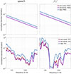 |
Figure 7. Normalized standard deviations of occlusion ratios, for PSD-based estimates of the occlusion effect (top) and TF-based estimates (bottom), for the ear from Figures 5 and 6. |
Using a coverage factor of two, i.e., defining the relevant uncertainty as twice the standard deviation, the resulting deviations of the occlusion ratio are seen to be lower than the critical value of 0.2 defined in Section 2.6.3, in particular at higher frequencies. Hence, random errors can be neglected except at low frequencies for the sung vowel.
The resulting normalized standard deviations of the occlusion ratios for TF-based measurements of the occlusion effect in the ear from Figures 5 and 6 are shown in the bottom two diagrams of Figure 7. Between about 200 Hz and about 3 kHz, the resulting uncertainty (given again by twice the normalized standard deviation of the occlusion ratio) is much lower than this value and hence, random errors can be neglected in this frequency range. Problems due to random errors on TF-based estimates are to be expected at frequencies below about 200 Hz for sung vowels, due to a lack of stimulus energy in this frequency range.
The results of the analysis of valid frequency ranges as outlined in Section 2.6.3 were finally applied to the computation of objective occlusion effects: in Figures 5d and 6d resulting occlusion effects are shown for all three variants of PSD-based and TF-based occlusion effect estimates: the sequential variants based on equation (6) (OEseq, PSDs) and equation (9) (OEseq, TFs), the simultaneous variants based on equation (7) (OEsim, device, PSDs) and the first equation of equation (10) (OEsim, device, TFs), and the alternative simultaneous variants based on equation (8) (OEsim, contraPSDs) and on the second equation of equation (10) (OEsim, contra, TFs). It can be seen that all three variants result in similar occlusion effects up to about 700 Hz. Above this frequency, the simultaneous variant that uses the sound pressure just outside the occluding device as reference becomes substantially larger than the two other variants, which can be partly attributed to the missing open ear gain, see Section 3.5.
3.2 Symmetry between test and reference ear in the open ear condition for all ears
Before proceeding to the analysis of occlusion effects in all 37 ears, the PSD level difference during voice production between the test ear and the reference ear in the open ear condition (measurement I in Fig. 4) is shown in Figure 8. This will give an indication to which extent the simultaneous method employing the contralateral sound pressure (Eq. (8)) will differ from the sequential method (Eq. (6)).
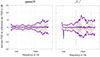 |
Figure 8. PSD level difference between test and reference ear in the open ear condition. Thin lines represent individual participants, thick lines 5- 50- and 95-percentiles of all level differences at frequencies where data from at least 10 participants were considered valid according to Section 2.6.3. |
For running speech (left diagram), no systematic difference can be observed. The inter-participant variability is symmetrical and rather low: from about 60 Hz to about 700 Hz, the range between the 5th and 95th percentiles of the level differences is mostly about ±1 dB, which then rises to about ±4 dB in the frequency region from 2.5 kHz to 5 kHz. Above 2 kHz, results from single pairs of ears exceed ±5 dB, but this occurs only sparsely. This result indicates that there is a high symmetry between the sound pressure PSDs in the two open ears during voice production.
Regarding systematic differences, this also holds for the sung vowel (right diagram). However, the inter-participant variability is considerably higher than for running speech, in particular at frequencies below about 1.5 kHz. Within this frequency range, the region between 500 Hz and 1500 Hz stands out with a remarkably increased inter-participant variability. Single pair results exceed ±5 dB from 400 Hz on. Above about 1500 Hz, the inter-participant variability is comparable to that of running speech. The higher inter-participant variability at frequencies below 1.5 kHz may be partly related to the spectral gap between the first two formants of /i:/. In addition, we suspect that differences in mouth opening (more pronounced when singing a vowel than when speaking normally) may contribute to this result.
3.3 Reproducibility of voice production in the open ear for all ears
In the sequential measurement of the occlusion effect, the participants were asked to produce own voice stimuli twice, in the open ear and in the occluded ear condition. Since the reference microphone in the open ear remained in place over these two conditions, the reproducibility of the own voice stimuli could be analyzed. This is shown in Figure 9. For running speech (left diagram), there is a slight systematic offset indicating that participants tended to speak more softly with one ear occluded. On the other hand, the inter-ear variability is moderately low, with a 5 to 95 percentile range of about ±2 dB to ±5 dB over the entire frequency range considered valid according to Section 2.6.3. Single ear results exceed ±5 dB differences only rarely. Running speech (of a familiar text) thus appears to be easy to reproduce, in spite of a change in the occlusion condition.
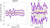 |
Figure 9. PSD level difference between condition I and II/III (Fig. 4) in the (open) reference ear. Thin lines represent individual ears, thick lines 5- 50- and 95-percentiles of all level differences at frequencies where data from at least 10 ears were considered valid according to Section 2.6.3. |
In contrast, sung vowels appear to be much more difficult to reproduce, see right diagram of Figure 9: there are systematic differences in the spectral fine structure and a large inter-ear variability, with the 5 to 95 percentile range exceeding ±5 dB and many ears exceeding ±10 dB in narrow frequency bands. The poor reproducibility for sung vowels, compared to reading a text, is not too surprising, given that none of the participants was a professional singer.
3.4 Measured occlusion effects in all ears
Figure 10 shows occlusion effects in all 37 ears, for all combinations of measurement method (i.e., sequential versus the two simultaneous variants, both PSD- and TF-based) and stimulus (running speech and sung vowel /i:/). Regarding median values of the occlusion effects, one can see that the sequential measurement and the simultaneous variant using the sound pressure in the open contralateral ear as reference are extremely similar, whereas the simultaneous variant using the sound pressure outside the occluding device results in higher median values of the occlusion effects above about 700 Hz. The differences between these variants are analyzed in more detail in Section 3.5 below.
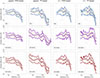 |
Figure 10. Measured occlusion effects in all 37 ears. Thin lines represent individual ears, thick lines 5- 50- and 95-percentiles of all level differences at frequencies where data from at least 10 ears were considered valid according to Section 2.6.3. Top: sequentially measured OEs (Eqs. (6), (9)), middle: simultaneously measured OEs using the device microphone as reference (Eq. (7) and first equation in Eq. (10)), bottom: simultaneously measured OEs using the probe tube microphone in the open contralateral ear as reference (Eq. (8) and second equation in Eq. (10)). |
The frequency range considered valid according to Section 2.6.3 extends to lower frequencies for running speech compared to the sung /i:/ and to higher frequencies for TF-based occlusion effects compared to PSD-based ones, in particular for running speech.
Regarding the inter-ear variability, TF-based estimates appear to result in a higher 5- to 95-percentile ranges than PSD-based ones. The difference between PSD-based and TF-based occlusion effects is discussed in more detail in Section 3.7 below.
3.5 Simultaneous versus sequential measurement of the occlusion effect in all ears
Figure 11 shows the differences between occlusion effects measured simultaneously and sequentially, using PSD-based measurements. In the top two diagrams, the focus is on the simultaneous variant with reference to the sound pressure just outside the occluding device. For both stimuli, the simultaneously measured occlusion effect appears to be systematically larger than the sequentially measured one up to about 500–700 Hz, by about 2 dB at 100 Hz. This systematic difference then decreases towards higher frequencies, before it increases rapidly above about 700 Hz to more than 15 dB at about 3 kHz. Data for individual ears deviate from this general trend by typically less than ±(2 − 3) dB for speech. For the sung vowel, the inter-ear variability is considerably higher, whereas the general trend is comparable to that of running speech.
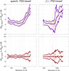 |
Figure 11. Differences between PSD-based occlusion effects measured simultaneously and sequentially, for all 37 ears. Thin lines represent individual ears, thick lines 5- 50- and 95-percentiles of all level differences at frequencies where data from at least 10 ears were considered valid according to Section 2.6.3. Top: simultaneous variant using the device microphone as reference (Eq. (7) and first equation in Eq. (10)), bottom: simultaneous variant using the probe tube microphone in the open contralateral ear as reference (Eq. (8) and second equation in Eq. (10)). |
In the two bottom diagrams of Figure 11, the analysis is repeated for simultaneous measurements with reference to the open contralateral ear. As could be expected, this is an almost exact copy of Figure 8, except that the valid frequency ranges are a little narrower since the validity criteria had to be satisfied not only for the open ear measurement, but also for the occluded ear measurement. In contrast to the two top diagrams, no systematic difference between simultaneously and sequentially measured occlusion effects can be seen throughout the valid frequency range. The inter-ear variability for speech is typically less than ±2 dB up to about 1000 Hz and increases to about ±4 dB at 3 kHz. For the sung vowel, it is again considerably higher.
3.6 Correcting the simultaneous measurement
The difference between the two simultaneous approaches observed in Section 3.5 above can be related to the gain provided by the sound transfer from the sound pressure at the (blocked) ear canal entrance to the sound pressure at the eardrum in the open ear, i.e., a variant of the open ear gain. This gain is known to provide an amplification of about 15 dB in the frequency range from 2 kHz to 5 kHz. We therefore corrected the simultaneously measured occlusion effect for every individual ear by subtracting the level of the transfer function of the sound pressure at the open eardrum, relative to that just outside the occluding device, for excitation by a loudspeaker in front of the participant.
This correction reduces the difference between the simultaneous and the sequential measurement of the occlusion effect to a certain degree, see Figure 12, but systematic differences persist, and the inter-ear variability is similarly high as before.
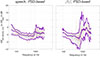 |
Figure 12. Same as the top row in Figure 11, but corrected for the open ear gain relative to the pressure just outside the occluding device for frontal loudspeaker excitation. |
3.7 TF-based versus PSD-based occlusion effects
Figure 13 shows differences between estimated occlusion effects based on TF versus PSD measurements, both for speech and for the sung vowel /i:/.
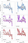 |
Figure 13. Differences between TF-based and PSD-based occlusion effects for all 37 ears. Thin lines represent individual ears, thick lines 5- 50- and 95-percentiles of all level differences at frequencies where data from at least 10 ears were considered valid according to Section 2.6.3. Top: sequentially measured OEs (Eqs. (6), (9)), middle: simultaneously measured OEs using the device microphone as reference (Eq. (7) and first equation in Eq. (10)), bottom: simultaneously measured OEs using the probe tube microphone in the open contralateral ear as reference (Eq. (8) and second equation in Eq. (10)). |
For running speech, the TF-based occlusion effect is in all variants, i.e., in the sequential and in both simultaneous ones, systematically larger than the PSD-based occlusion effect at low frequencies up to about 1–2 kHz. Above 2 kHz, the TF-based occlusion effect is systematically lower than the PSD-based one. The inter-ear variability of this level difference is asymmetrical, in that TF-based estimates are more often larger than PSD-based ones. The 5 to 95 percentile range is particularly large at frequencies below 150 Hz as well as around 350 Hz, 900 Hz and 2300 Hz. Here, we should recall that the inter-ear variability of the occlusion effect was found to be higher for TF-based measurements than for PSD-based ones, especially around 900 Hz, see Figure 10.
In contrast to the findings with running speech, no discernible systematic discrepancy was observed between the TF-based and the PSD-based occlusion effect for the sung vowel at low frequencies up to about 600 Hz. Between 600 and 2 kHz, the TF-based occlusion effect is, however, again systematically higher than the PSD-based one. In addition, the inter-ear variability is increased in this frequency range. We note again that this frequency range coincides with the spectral gap between the first two formants of /i:/.
These results confirm the interpretation from the example ear in Section 2, namely that running speech induces a time-variant fluctuation of the occlusion effect which leads to a systematic difference between TF-based and PSD-based estimates. For single (sung) vowels, this effect is strongly reduced, but TF-based estimates still tend to result in a larger inter-ear variability than PSD-based ones, see Figure 10.
4 Discussion
4.1 Time variance of the occlusion effect
As already mentioned in Section 3.1, it is not surprising to observe a time-varying behavior of the occlusion effect for running speech. For vowels, it is well-known that the strength of the occlusion effect depends on the vowel being produced: it is largest for closed vowels such as /i:/ and smallest for open vowels such as /a:/ [3, 4]. In consequence, one must expect a varying strength of the occlusion effect in running speech where different vowels are produced successively. The perceptual consequences of a time-variant occlusion effect are, on the other hand, much less well known but may potentially have a large impact on mitigation strategies: it remains in particular unclear whether the subjective annoyance is dominated by an average (or other statistic) over time-variant fluctuations or whether it fluctuates itself. The latter would motivate the use of time-variant active control strategies as proposed, e.g., by Ohlenbusch et al. [8]. The preference for passive, static measures such as vents or earpiece surface profiling in hearing aids and ear protection devices appears thus to be rather driven by practical considerations which may need to be reconsidered for modern hearables.
4.2 Stimulus duration and bandwidth considerations
Of the own-voice stimuli considered in this study, running speech lasted longer (with a mean of 38 s of cut material) than sung vowels (mean of 10.5 s of cut material). This resulted in lower random errors in spectral estimates for speech compared to sung vowels (see Fig. 7). In the current study, this effect could be neglected since random errors were predicted to be sufficiently low, except at very low and very high frequencies. Note, however, that random errors also depend on the chosen bandwidth of the spectral smoothing: they may become important if higher spectral resolution is desired.
Speech stimuli also exhibited a wider bandwidth than sung vowels, in particular towards low frequencies, and, to a lesser degree, towards high frequencies as well (see Fig. 10). The additional low-frequency content of speech in comparison to sung vowels was at first sight surprising, but can be explained by the presence of natural variations in the fundamental frequency and by broadband consonants in running speech. In addition, occlusion effects estimated from sung vowels were affected by the spectral gap between the first two formants (see Fig. 6).
Running speech was also easier to reproduce than sung vowels in subsequent trials (see Sect. 3.3). This confirms conclusions by Hansen [19], Section 7.3, who also found a higher reproducibility with running speech compared to vowels. In addition, speech is likely the most ecologically valid stimulus.
4.3 Simultaneous versus sequential measurement of the occlusion effect
Our findings of a systematic overestimation of the occlusion effect when using simultaneous measurements with reference to the sound pressure outside the occluding device agree partly with the results from Saint-Gaudens et al. [20], in that the difference between the two methods gets larger above about 700 Hz (they found 800 Hz), and in that the reference to the open contralateral ear is unaffected throughout the entire frequency range they considered (from 160 Hz to 2 kHz).
However, Saint-Gaudens et al. [20] found both small over- and underestimations with the method using the sound pressure outside the occluding device as a reference at frequencies below 800 Hz and concluded that this method would be well-suited for clinical and field assessments. In contrast, systematic overestimations were found in the present study at virtually all frequencies, both for running speech and for /i:/ (Fig. 11). A possible explanation for this discrepancy is that we found the most important low-frequency overestimations below 300 Hz where Saint-Gaudens et al. [20] only analyzed two frequency bands (160 Hz and 250 Hz) in which they actually also reported a systematic overestimation (see their Fig. 9) but did not specifically discuss it. In addition, the in-ear device used in the current study was vented, unlike the device used by Saint-Gaudens et al. [20], which may also have contributed to the observed mismatch at low frequencies, for instance by sound leaking in and out of the vent, or by effects related to the lower overall occlusion generated by vented earpieces.
Furthermore, we did not observe the same increase in inter-ear variability with the sequential method that Saint-Gaudens et al. [20] reported for sustained vowels. This may be explained by the poor reproducibility of vowel spectra together with only monitoring the overall level in their work, whereas in the present study, we used measured reference spectra.
4.4 High-frequency correction of the “sim, device" method
In line with the results from Saint-Gaudens et al. [20], we observed a large discrepancy between occlusion effects measured with the “device" variant of the simultaneous method in comparison to the sequential method at frequencies above 700 Hz, see Section 3.5. As mentioned earlier, this discrepancy can be explained by the missing (modified) open ear gain in the simultaneous measurement.
However, our attempt to compensate for the missing open ear gain by measured transfer functions with frontal loudspeaker excitation was only partly successful and inferior to the “contra" variant of the simultaneous method, in particular for the sung vowel, see Section 3.6. This indicates that frontal (far-field) loudspeaker excitation is not a perfect surrogate for own-voice excitation when characterizing the level difference between open ear and blocked ear sound pressure spectra. Different factors contribute to this lack of success, including the interplay between voice directivity and the direction-dependence of the open ear gain, the absence of body-conducted own-voice components in the open ear condition, and the fact that even more spectral estimates are included, each adding errors to the final estimates of the occlusion effect. Possibly, a less elevated frontal loudspeaker position could be beneficial, since the mouth is lower than the ear. This remains, however, to be investigated.
4.5 PSD-based versus TF-based measurement of the occlusion effect
In the current study, no convincing benefit of using TF-based estimates over the more traditional PSD-based estimates of the occlusion effect was found. This was not expected since, theoretically, TF-based estimates may work at low or even negative SNRs. To benefit from this property, the disturbances must be stationary and their PSDs must be known accurately. Neither of these requirements can be guaranteed under the measurement conditions considered here.
Still, applying the criteria for valid frequency ranges developed in Section 2.6.3, one can indeed observe an increased frequency range of TF-based occlusion estimates in comparison to PSD-based estimates when the stimulus is running speech. However, the criteria for valid frequency ranges from Section 2.6.3 explicitly exclude systematic errors due to time-variant effects and must therefore be used with much caution. As an example, systematic differences between TF- and PSD-based estimates of the occlusion effect for speech were observed up to about 3 kHz (see Fig. 13). It is highly speculative to make assumptions for higher frequencies where PSD-based estimates were defined as invalid.
In summary, since the annoyance perception can be assumed to be related to the sound pressure PSD at the eardrum, PSD-based estimates of the occlusion effect should be preferred.
5 Conclusions
One’s own voice is a challenging test signal. It is often poorly reproducible, has a limited bandwidth, and is therefore affected by poor SNRs, and it influences the system we try to measure in a time-variant manner. When measuring the objective occlusion effect, all of the above issues have to be taken into account. The relative importance of each of them further depends on the stimulus one is trying to generate with the own voice.
For running speech, the time variance of the occlusion effect induced by the succession of different phonemes is the most critical issue. This leads to systematic differences in the occlusion effect when the latter is measured by PSDs versus by TFs. On the other hand, running speech extends to quite low frequencies (about 60 Hz) and gives acceptable SNRs up to about 5 kHz in the open ear and up to about 3 kHz in the occluded ear. In addition, it is fairly well reproducible.
For sung vowels, time-variant occlusion effects are negligible. However, there are SNR problems, especially at low frequencies and in spectral gaps between the formants. The high-frequency limit appears to be similar to the one for running speech. Sung vowels are much harder to reproduce than running speech.
The popular method of measuring the occlusion effect by simultaneously measuring inside and outside the occluding device entails systematic errors of up to about 3 dB to 4 dB in vented earpieces, even in the frequency range in which it was previously considered valid, and differences of 10 dB to 15 dB above approximately 700 Hz, due to the absent open ear gain. Correcting this method by using the (modified) open ear gain for frontal loudspeaker excitation reduces errors above 1 kHz, but a systematic positive error persists.
In contrast, the simultaneous measurement with reference to the open contralateral ear is accurate throughout the frequency range in which an acceptable SNR is achieved. Furthermore, simultaneous methods bypass issues related to own-voice reproducibility between recording conditions.
The use of TF-based estimates of the occlusion effect results in more problems than advantages in comparison to PSD-based estimates. In particular, it is sensitive to the time variance of the occlusion effect, and it results in a higher inter-ear variability of the occlusion effect.
The perceptual consequences of a time-variant occlusion effect are not well understood, but need to be taken into account for successful occlusion control strategies.
Acknowledgments
We would like to thank our participants for their patience and efforts. We also thank the three anonymous reviewers for helpful comments on an earlier version of the manuscript.
Funding
This research was partially funded by Deutsche Forschungsgemeinschaft (DFG, German Research Foundation) – Project ID 352015383 – SFB 1330 A4 and C1.
Conflicts of interest
The authors have no conflicts to disclose.
Data availability statement
Data are available on request from the authors.
Ethics approval
All experimental procedures were approved by the University of Oldenburg Ethics Committee under reference Drs.EK/2021/064 and conducted in accordance with the principles outlined in the WMA Declaration of Helsinki. All participants were informed of the potential risks and provided their informed consent prior to participation.
References
- G.V. Békésy: The structure of the middle ear and the hearing of one’s own voice by bone conduction. The Journal of the Acoustical Society of America 21, 3 (1949) 217–232. [Google Scholar]
- C. Pörschmann: Influences of bone conduction and air conduction on the sound of one’s own voice. ACUSTICA/Acta Acustica 86, 6 (2000) 1038–1045. [Google Scholar]
- T. Zurbrügg, A. Stirnemannn, M. Kuster, H. Lissek: Investigations on the physical factors influencing the ear canal occlusion effect caused by hearing aids. Acta Acustica united with Acustica 100, 3 (2014)527–536. [Google Scholar]
- M. Killion: The hollow voice occlusion effect, in: Proceedings of 13th Danavox Symposium, 1988, pp. 231–241. [Google Scholar]
- M. Blau, T. Sankowsky, H. Oberdanner, A. Stirnemann: Einfluss des Otoplastikprofils auf den objektiven Okklusionseffekt [influence of the earmold profile on the objective occlusion effect], in: Fortschritte der Akustik – DAGA 2008, Dresden, 2008. [Google Scholar]
- F. Denk, T. Hieke, M. Roberz, H. Husstedt: Occlusion and coupling effects with different earmold designs – all a matter of opening the ear canal? International Journal of Audiology 62, 3 (2023) 227–237. [CrossRef] [PubMed] [Google Scholar]
- F. Kuk, D. Keenan, C.-C. Lau: Vent configurations on subjective and objective occlusion effect. Journal of the American Academy of Audiology 16, 9 (2005) 747–762. [Google Scholar]
- M. Ohlenbusch, C. Rollwage, S. Doclo: Modeling of speech-dependent own voice transfer characteristics for hearables with an in-ear microphone. Acta Acustica 8 (2024) 28. [Google Scholar]
- K. Carillo, O. Doutres, F. Sgard: On the removal of the open earcanal high-pass filter effect due to its occlusion: a bone-conduction occlusion effect theory. Acta Acustica 5 (2021) 36. [Google Scholar]
- R. Carle, S. Laugesen, C. Nielsen: Observations on the relations among occlusion effect, compliance, and vent size. Journal of the American Academy of Audiology 13 (2002) 25–37. [Google Scholar]
- S. Laugesen, N.S. Jensen, P. Maas, C. Nielsen: Own voice qualities (OVQ) in hearing-aid users: there is more than just occlusion. International Journal of Audiology 50, 4 (2011) 226–236. [Google Scholar]
- J. Kiessling, B. Brenner, C.T. Jespersen, J. Groth, O.D. Jensen: Occlusion effect of earmolds with different venting systems. Journal of the American Academy of Audiology 16, 4 (2005) 237–249. [Google Scholar]
- H. Dillon: Hearing Aids. Thieme Medical Publishers, 2012. [Google Scholar]
- T. Jürgens, P. Ihly, J. Tchorz, T. Nishiyama, C. Tanaka, D. Suzuki, S. Shinden, T. Kitama, K. Ogawa, J. Zaar, S. Laugesen, G. Jones, M. Vatti, S. Santurette: Closedness of acoustic coupling and audiological measures are associated with individual speech-in-noise benefit from noise reduction in hearing aids. Trends in Hearing 29 (2025) 23312165251325983. [Google Scholar]
- A. Winkler, M. Latzel, I. Holube: Open versus closed hearing-aid fittings: a literature review of both fitting approaches. Trends in Hearing 20 (2016) 233121651663174. [Google Scholar]
- S. Liebich, P. Vary: Occlusion effect cancellation in headphones and hearing devices – the sister of active noise cancellation. IEEE/ACM Transactions on Audio, Speech, and Language Processing 30 (2021) 35–48. [Google Scholar]
- F. Denk, L. Jürgensen, H. Husstedt: Evaluation of active occlusion effect cancellation in earphones by subjective, real-ear and coupler measurements. Journal of the Audio Engineering Society 72, 3 (2024)145–159. [Google Scholar]
- K.A. Vasil-Dilaj, K.M. Cienkowski: The influence of receiver size on magnitude of acoustic and perceived measures of occlusion. American Journal of Audiology 20 (2011) 61–68. [Google Scholar]
- M.Ø. Hansen: Occlusion effects, Part I: hearing aid users experiences of the occlusion effect compared to the real ear sound level, Vol. report 71. Department of Acoustic Technology, Technical University of Denmark, Lyngby, Denmark, 1997. [Google Scholar]
- H. Saint-Gaudens, H. Nélisse, F. Sgard, O. Doutres: Towards a practical methodology for assessment of the objective occlusion effect induced by earplugs. The Journal of the Acoustical Society of America 151, 6 (2022) 4086–4100. [Google Scholar]
- A. Bernier, J. Voix: An active hearing protection device for musicians, in: Proceedings of 21st International Congress on Acoustics, Montreal (Canada), 2013, pp. 040015–040015. [Google Scholar]
- R.E. Bouserhal, A. Bernier, J. Voix: An in-ear speech database in varying conditions of the audio-phonation loop. The Journal of the Acoustical Society of America, 145, 2 (2019) 1069–1077. [Google Scholar]
- J. Mejia, H. Dillon, M. Fisher: Active cancellation of occlusion: an electronic vent for hearing aids and hearing protectors. The Journal of the Acoustical Society of America 124, 1 (2008) 235–240. [Google Scholar]
- M.C. Killion: Occlusion meter and associated method for measuring the occlusion of an occluding object in the ear canal of a subject. US Patent 5,577,511, 1996. [Google Scholar]
- F. Denk, M. Lettau, H. Schepker, S. Doclo, R. Roden, M. Blau, Wellmann, J. Blau, B. Kollmeier: A one-size-fits-all earpiece with multiple microphones and drivers for hearing device research, in: Audio Engineering Society Conference: 2019 AES International Conference on Headphone Technology. Audio Engineering Society, 2019. [Google Scholar]
- J.S. Bendat, A.G. Piersol: Random Data: Analysis and Measurement Procedures, 2nd edn. John Wiley & Sons, 1986. [Google Scholar]
- A.L. Wicks, H. Vold: The Hs frequency response function estimator, in: Proceedings of the 4th International Modal Analysis Conference, Los Angeles, CA, USA. Vol. 2, 1986, pp. 897–899. [Google Scholar]
- A. Potchinkov: Measurement of frequency responses of nonlinearly distorted SISO systems in noisy environments with generalized parameter frequency response estimators. Signal Processing 86, 8 (2006) 2094–2114. [Google Scholar]
- IPA: Handbook of the International Phonetic Association: A guide to the use of the International Phonetic Alphabet. Cambridge University Press, 1999. [Google Scholar]
- M.S. Puckette: Pure data: another integrated computer music environment, in: Proceedings of the International Computer Music Conference, San Francisco (USA), 1996. [Google Scholar]
- M. Blau: Acoustical measurements for everyone, in: Proceedings of Internoise ’05, Rio de Janeiro (Brazil), 2005. [Google Scholar]
- P.D. Welch: The use of fast fourier transform for the estimation of power spectra: a method based on time averaging over short, modified periodograms. IEEE Transactions on Audio and Electroacoustics 15, 2 (2023) 70–73. [Google Scholar]
- P.D. Hatziantoniou, J.N. Mourjopoulos: Generalized fractional-octave smoothing of audio and acoustic responses. Journal of the Audio Engineering Society 48, 4 (2000) 259–280. [Google Scholar]
- J.S. Bendat: Statistical errors in measurement of coherence functions and input/output quantities. Journal of Sound and Vibration 59, 3 (1978) 405–421. [Google Scholar]
Cite this article as: Blau M. Roden R. Hauenschild N. Kersten S. Rehman R. Vorländer M. & Fels J. 2025. Methods to experimentally characterize the own-voice-generated objective occlusion effect induced by hearables. Acta Acustica, 9, 73. https://doi.org/10.1051/aacus/2025055.
All Figures
|
Figure 1. Illustration of the occlusion effect: by occluding the ear, the eardrum sound pressure changes from pe, open to pe, occl. |
| In the text | |
|
Figure 2. Signal model of the objective occlusion effect, including a reference path: x is the unobservable excitation by one’s own voice, which may change in every condition. p r and p e are the reference and eardrum sound pressures, respectively. m and n are uncorrelated noise signals representing background noise and other disturbances on the measured sound pressure signals. |
| In the text | |
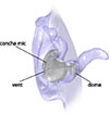 |
Figure 3. In-ear hearing device used in this study, cf. Denk et al. [25]. |
| In the text | |
|
Figure 4. Open and occluded ear conditions investigated in this study: (I) both ears open, with probe tube microphones at each eardrum, (II) and (III) one ear occluded, one open, probe tube microphones as in I. |
| In the text | |
|
Figure 5. Example of measured PSDs, TFs, derived occlusion effects and MSCs in the left ear of one participant producing running speech. Column (a): both ears open (open ear condition in the sequential measurement), column (b): ipsilateral ear occluded (occluded ear condition used in both the sequential and the simultaneous measurements), column (c): same as (b), but the reference changed from the contralateral sound pressure to the ipsilateral sound pressure outside the device (simultaneous measurement), column (d): derived occlusion effects: PSD-based (top) and TF-based (bottom). |
| In the text | |
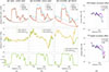 |
Figure 6. Same as Figure 5, but for a sung vowel (/i:/). Noise PSDs were taken from Figure 5. |
| In the text | |
|
Figure 7. Normalized standard deviations of occlusion ratios, for PSD-based estimates of the occlusion effect (top) and TF-based estimates (bottom), for the ear from Figures 5 and 6. |
| In the text | |
|
Figure 8. PSD level difference between test and reference ear in the open ear condition. Thin lines represent individual participants, thick lines 5- 50- and 95-percentiles of all level differences at frequencies where data from at least 10 participants were considered valid according to Section 2.6.3. |
| In the text | |
|
Figure 9. PSD level difference between condition I and II/III (Fig. 4) in the (open) reference ear. Thin lines represent individual ears, thick lines 5- 50- and 95-percentiles of all level differences at frequencies where data from at least 10 ears were considered valid according to Section 2.6.3. |
| In the text | |
|
Figure 10. Measured occlusion effects in all 37 ears. Thin lines represent individual ears, thick lines 5- 50- and 95-percentiles of all level differences at frequencies where data from at least 10 ears were considered valid according to Section 2.6.3. Top: sequentially measured OEs (Eqs. (6), (9)), middle: simultaneously measured OEs using the device microphone as reference (Eq. (7) and first equation in Eq. (10)), bottom: simultaneously measured OEs using the probe tube microphone in the open contralateral ear as reference (Eq. (8) and second equation in Eq. (10)). |
| In the text | |
|
Figure 11. Differences between PSD-based occlusion effects measured simultaneously and sequentially, for all 37 ears. Thin lines represent individual ears, thick lines 5- 50- and 95-percentiles of all level differences at frequencies where data from at least 10 ears were considered valid according to Section 2.6.3. Top: simultaneous variant using the device microphone as reference (Eq. (7) and first equation in Eq. (10)), bottom: simultaneous variant using the probe tube microphone in the open contralateral ear as reference (Eq. (8) and second equation in Eq. (10)). |
| In the text | |
|
Figure 12. Same as the top row in Figure 11, but corrected for the open ear gain relative to the pressure just outside the occluding device for frontal loudspeaker excitation. |
| In the text | |
|
Figure 13. Differences between TF-based and PSD-based occlusion effects for all 37 ears. Thin lines represent individual ears, thick lines 5- 50- and 95-percentiles of all level differences at frequencies where data from at least 10 ears were considered valid according to Section 2.6.3. Top: sequentially measured OEs (Eqs. (6), (9)), middle: simultaneously measured OEs using the device microphone as reference (Eq. (7) and first equation in Eq. (10)), bottom: simultaneously measured OEs using the probe tube microphone in the open contralateral ear as reference (Eq. (8) and second equation in Eq. (10)). |
| In the text | |
Current usage metrics show cumulative count of Article Views (full-text article views including HTML views, PDF and ePub downloads, according to the available data) and Abstracts Views on Vision4Press platform.
Data correspond to usage on the plateform after 2015. The current usage metrics is available 48-96 hours after online publication and is updated daily on week days.
Initial download of the metrics may take a while.